Development of Visual Servoing-Based Autonomous Docking Capabilities in a Heterogeneous Swarm of Marine Robots

Abstract

This paper describes the design, development, and testing of both hardware and software for a visual servoing-based system that enables agents within a heterogeneous marine robotic swarm to share energy. The goal of this system is prolonging the active operational time of the swarm as a whole, allowing it to perform long-term environmental monitoring and data collection missions. The implementation presented in the paper features an over-actuated autonomous surface platform docking up to four floating sensor nodes at a time and replenishing their batteries using wireless inductive charging. Mechanical solutions for each robot segment related to the docking procedure are presented, along with pertinent high-level and low-level control structures. A node featuring an extended Kalman filter and additional heuristics is used to fuse measurements from a neural network trained for object detection and a hue thresholding image processing algorithm, in order to track the docking target and achieve visual servoing. Finally, experimental results in both a controlled environment and challenging conditions on-site are presented. Once deployed, the developed system successfully enables the approach and docking of the designated target, showing its feasibility in different real-life conditions.

1. Introduction

The EU Horizon 2020 FET project subCULTron aims to develop a heterogeneous swarm of marine robots and deploy it on an unsupervised mission of long-term marine monitoring and exploration in the challenging environment of the lagoon surrounding Venice, Italy [1,2]. The system consists of multiple robotic agents of three distinct types, and was envisioned as an artificial marine ecosystem. The three agent types are as follows: five over-actuated autonomous surface vehicles (ASV) called aPads or artificial lily pads; a small swarm of highly mobile aFish or artificial fish; and 120 underwater sensor nodes with limited mobility called aMussels, or artificial mussels. This paper focuses on an algorithm developed primarily for interaction between the aPad and aMussel agent types.

The aPad (Figure 1) is a modular robotic platform with powerful batteries, an X-shaped thruster configuration which makes it highly maneuverable, and the highest computational power in the swarm. Equipped with mechanical docking stations and inductive charging coils, one of the aPad’s main roles and most important abilities is to transport and wirelessly charge up to four other swarm agents at a time. With its wireless router, two antennas, and an acoustic modem, it also plays an important role in the swarm’s communication structures and possible underwater-swarm-to-surface-observer information transfer.

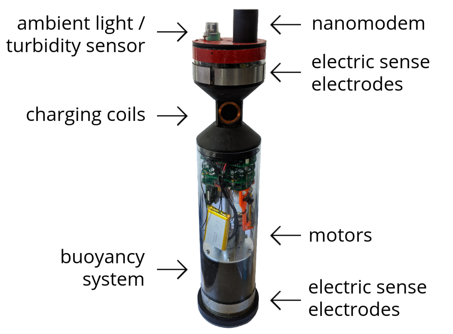
The aMussel (Figure 2) carries a wide selection of sensors, including temperature, pressure, turbidity, ambient light, and dissolved oxygen. It has very limited movement capabilities, equipped only with a variable buoyancy system consisting of a piston and diaphragm which allows it to float to the water’s surface, sink to the sea bed, or stay hovering at a set depth. For deployment and relocation to specific points in its environment, the aMussel requires the help of the aPad. Once deployed, the numerous aMussels use the miniaturized acoustic modems mounted on their top caps to function as an underwater acoustic sensor network (UASN) on a mission of long-term data collection and environmental observation.

To achieve long-term autonomy necessary for the completion of its monitoring mission, energy sharing within the subCULTron heterogeneous robotic swarm has been a key part of the design and development of the system as a whole. The primary goal is to have the aPad surface platform that is quite energy-rich transfer some of its energy to the much more limited aMussel, using specially designed hardware and software solutions. The initial implementation of the energy sharing system, as well as the results of some early proof-of-concept experiments, have been described in [4].

Autonomous underwater vehicle (AUV) docking is a concept often explored in the literature, and an important part of marine operations. Recently, Ref. [5] gave an overview of autonomous docking of AUVs with an underwater station, highlighting and examining the most frequently used mechanical docking concepts as well as navigation, guidance, and control methodologies. Adaptive and robust solutions are sought after, due to the need for the systems to perform well in a variety of conditions in the field. Fuzzy logic is frequently used for this purpose, especially as a mechanism to handle unknown disturbances such as water currents, for example in [6,7]. Several reinforcement learning strategies are studied in the context of underwater AUV docking, and compared with classical and optimal control techniques in [8]. Computer vision plays a large role in many docking approaches, such as in [9], where an AUV homes in on four markers placed around a docking station using a system of two cameras, combining binocular and monocular vision positioning methods. In [10] authors present ASV/AUV coordination to achieve docking based on a visual estimate, while in [11] visual-based pose estimation techniques are used to dock a work-class remotely operated vehicle (ROV) with both static and dynamic docking stations.

Mechanical design that complements the docking function or even a specific vehicle shape is necessary in real working conditions. Due to standard AUV hull shapes, this often means a funnel or cone-shaped system [12]. In [13], a system combining existing static cabled ocean observatory network structures and AUVs is described, in which the long-term mission capabilities of the AUV are enhanced. The authors of [14] describe an underwater wireless charging system consisting of a station which vehicles navigate to recharge their batteries and extend their data gathering capabilities. In [15] the authors propose a three-phase wireless charging system that could be used in a field-deployable charging station capable of rapid, efficient, and convenient AUV recharging during or in between missions, while taking care not to affect the instrumentation in the AUV itself.

In the case of the subCULTron swarm, the “docking station” is an ASV—the aPad—bearing four docking mechanisms, and it navigates to and docks the AUV—the aMussel—since the agent requiring charge has limited movement capabilities beyond the vertical. A funnel-like shape is used on the aMussel top cap, while the aPad dock consists of two prongs and a servo-powered latch. The subCULtron swarm uses non-contact power transmission via inductive coil coupling, while bespoke mechanical design ensures coil alignment for maximizing efficiency.

Although the main purpose of docking stations is battery recharge, also relevant is data and mission configuration download and upload without a need for vehicle recovery [16]. In the system described in [17], two modes of communication are employed: acoustic communication for long ranges and optical for short ranges. Both in this monitoring system and the one given in [18], fixed underwater sensors collect data about the environment while AUVs act as communication relays periodically delivering the data to the surface. In contrast to these approaches, the subCULtron swarm is fully reconfigurable, and the aPads, taking on the role of communication relays, remain on the surface ready to transfer information at all times. While underwater, aMussels communicate with them using acoustic modems, and when surfaced and docked, the aMussels upload collected data logs to the aPads using WiFi.

As opposed to more traditional docking/charging stations and more similar to approaches used in the subCULTron swarm, Ref. [19] proposes an autonomous mobile charger robot which acts within the swarm, monitors the other agents’ location and battery level, and seeks out low-powered agents to respond to their charging requests. Robots in need of charging approach the charging robot and dock to one of its several charging stations. It also contains algorithms developed for cooperation between robots in need of charging and the robot carrying the charging stations. In [20] specialized agents serve as the starting points of energy supply chains within a robotic swarm.

The algorithm proposed and implemented here is an image-based visual servoing variant (IBVS) with end-point closed-loop control, since the visual sensor moves together with the effector towards the target, while itself integrated into the control loop of the system. The information about various offsets within the image acquired from the image processing segments of the algorithm is used directly in the control algorithm to calculate reference signals, as opposed to being used as a basis for estimating the real-world 3D space position or pose of the target. This is a classical, well-established and well-documented approach, as seen in [21,22,23]. More recently, applications of various implementations of visual servoing in the field of marine robotics can be seen in [24], where a visual servo control approach was successfully transferred from an industrial manufacturing context to underwater robotics tasks autonomously performed by a subsea hydraulic manipulator mounted on a work-class ROV. In [25], visual servoing is used as a method of achieving station-keeping in an underwater environment, with unmarked natural features acting as targets for the image tracking algorithm and enabling an unmanned underwater vehicle (UUV) to hover above planar targets on the sea bed. In [26], a more complex hierarchical control structure featuring visual servoing is introduced to achieve dynamic positioning of a fully actuated underwater vehicle.

Recent related work [27] is focused on the analysis and improvement of long-term autonomy of the subCULTron system, in particular by using the potential of the energy exchange capabilities between aPad and aMussel robots. The paper focuses on efforts to create a means of studying the effects of decision-making and scheduling algorithms in a logistically viable way, and also describes data acquisition experiments performed during efforts to model subCULTron swarm agent batteries as well as validate the long-term potential of the agents thanks to low-power and sleep modes of operation.

Due to the limited processing power of swarm agents, and taking into account minimizing energy consumption as an important goal during long-term swarm operations, approaches to both hardware and software design in the subCULTron swarm needed to be simple yet effective. This paper presents an overview of in-house developed hardware and software with the purpose of enabling autonomous docking between different agents in the robotic swarm using a visual servoing approach and fusing the results of classical image processing methods and a neural network trained for object detection. It also describes several successfully performed real-world marine environment trials with completely autonomous agent cooperation resulting in successful wireless energy transfer in different conditions.

The paper is organized as follows: Section 2 describes the development of the system, with Section 2.1 focusing on the evolution of the mechanical segments of the aMussel and aPad robots relevant to the docking algorithm, and Section 2.2 describing the software segment and overall control structure of the developed system and giving insight into its lower-level controllers for surge and yaw speeds. Section 2.3 gives an overview of image processing algorithms and models used to achieve object recognition and visual servoing. Section 2.4 describes the docking system implementation of a filter node featuring an extended Kalman filter for sensor fusion and object tracking. Section 3 contains a detailed writeup of a structured docking experiment in controlled conditions and an experiment undertaken in challenging real-world conditions, including results and commentary. Finally, some conclusions on the work are drawn in Section 4.

2. Materials and Methods

2.1. Mechanical System Design

The mechanical systems, hardware, and software necessary for autonomous docking have all gone through several iterations of development, testing, and redesign, though the basic concept has remained the same throughout: the aPad seeks the recognizable top cap of a floating aMussel using a visual sensor, approaches it using a control algorithm-based around visual servoing, moving so the aMussel docking section is aligned with the aPad docking mechanism, then finally activates the docking mechanism to secure the aMussel in place so wireless charging using inductive coils can take place.

The three main components of the docking procedure are the aMussel top cap, the aPad visual sensor, and the aPad docking unit, which will be examined in the following subsections.

2.1.1. aMussel Top Cap

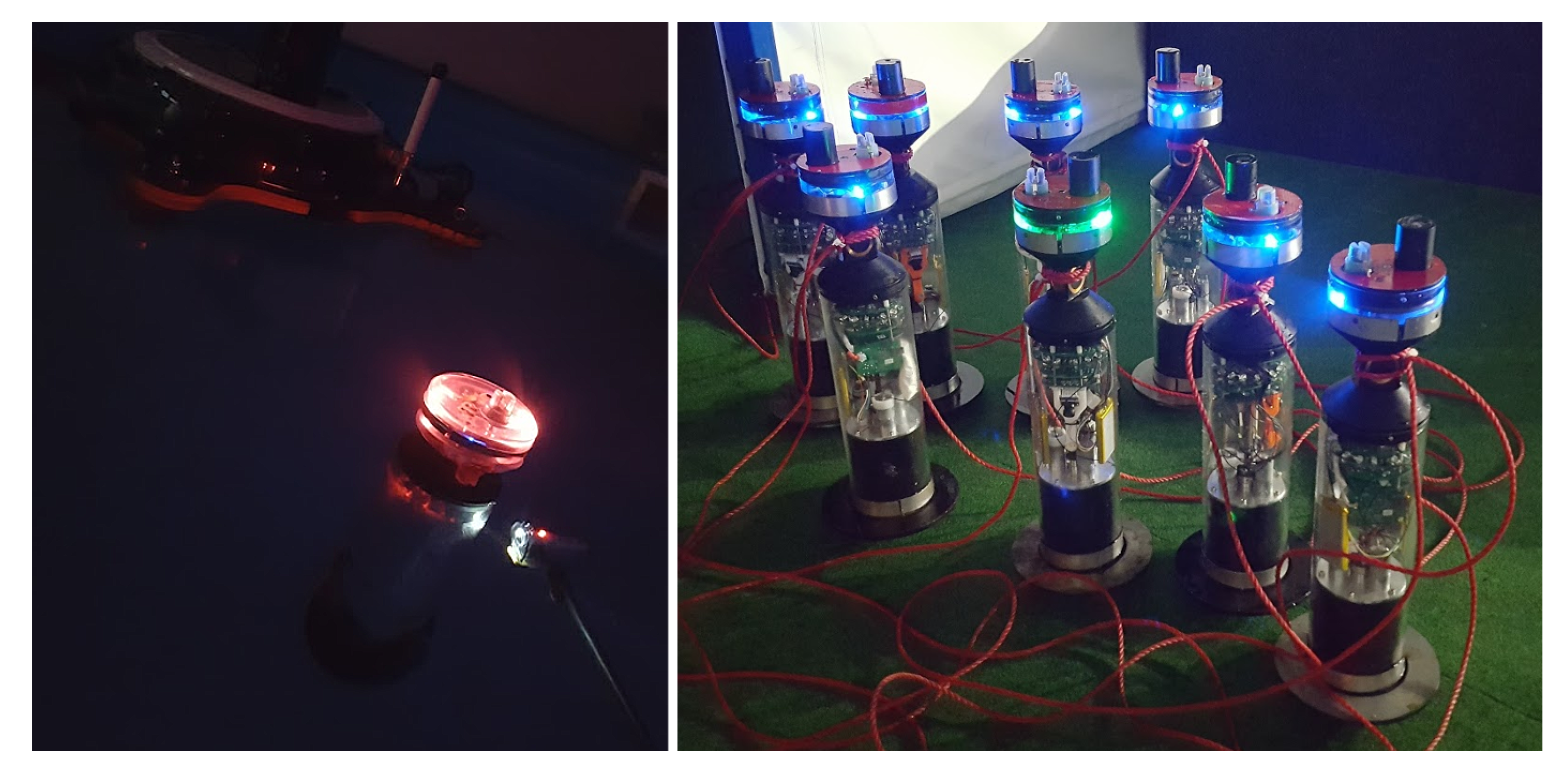
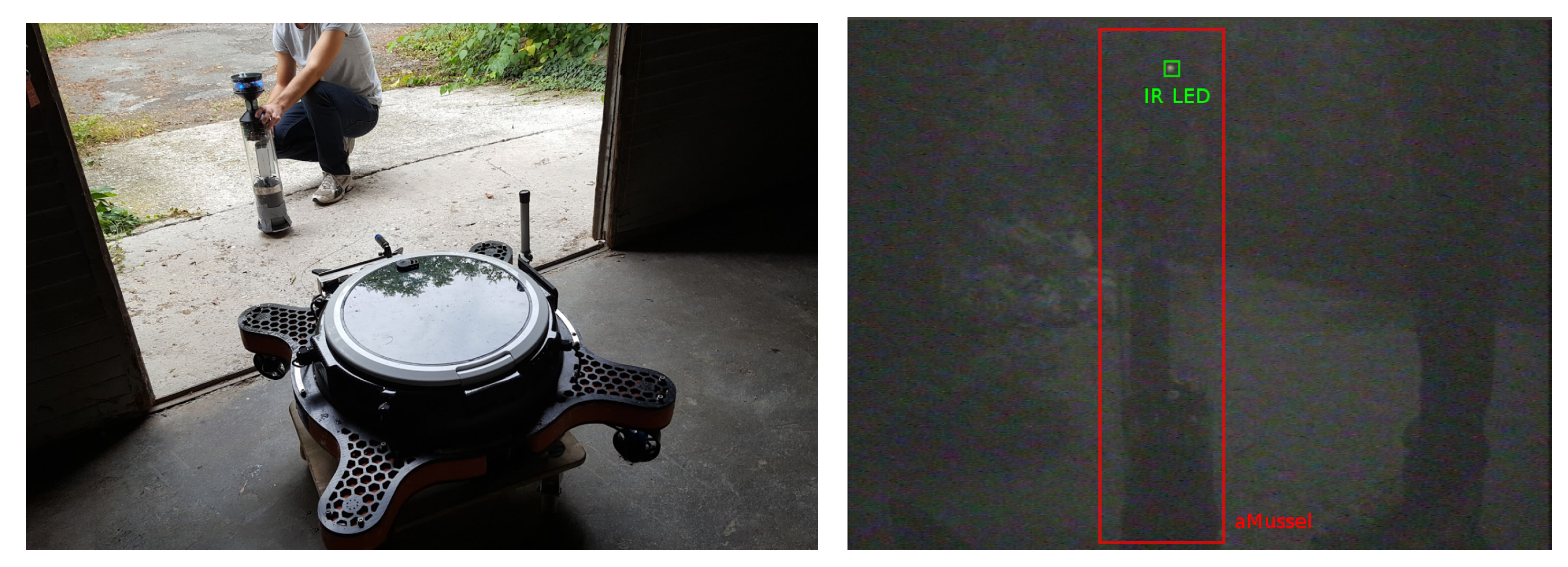
In the erstwhile docking concept, the aMussel was an active participant throughout. The original aMussel top cap prototype had IR LEDs included for the docking camera to home in on, thanks to a covering of IR filter film over its lens (for an example of the view through the IR filter, see Figure 3). The three high intensity wide-angle (OptiTrack) IR LEDs were mounted evenly spaced within the cap around its perimeter, to ensure aMussel visibility from all angles. The aMussel turned these LEDs on and off on demand, making it in essence an active beacon.

This design was changed to make the aMussel a more passive agent during the docking process as well as to ease aMussel production. Its IR LEDs were replaced with a covering of reflective tape which is saturated red when viewed using a normal RGB camera, and brightly reflective when viewed through an IR filter. Now, after it sends out its docking request, an aMussel no longer has to keep any LEDs powered—in fact, it does not have to be turned on at all, leading to power conservation and fewer concerns about maintaining battery level above a certain threshold, as an aMussel can still be picked up by an aPad without issue even if its battery completely runs out. The aPad is the only active agent in the redesigned docking process, as both the IR emitter and receiver are entirely on its end. Original and redesigned aMussel top caps are shown in Figure 4.

2.1.2. aPad Visual Sensor

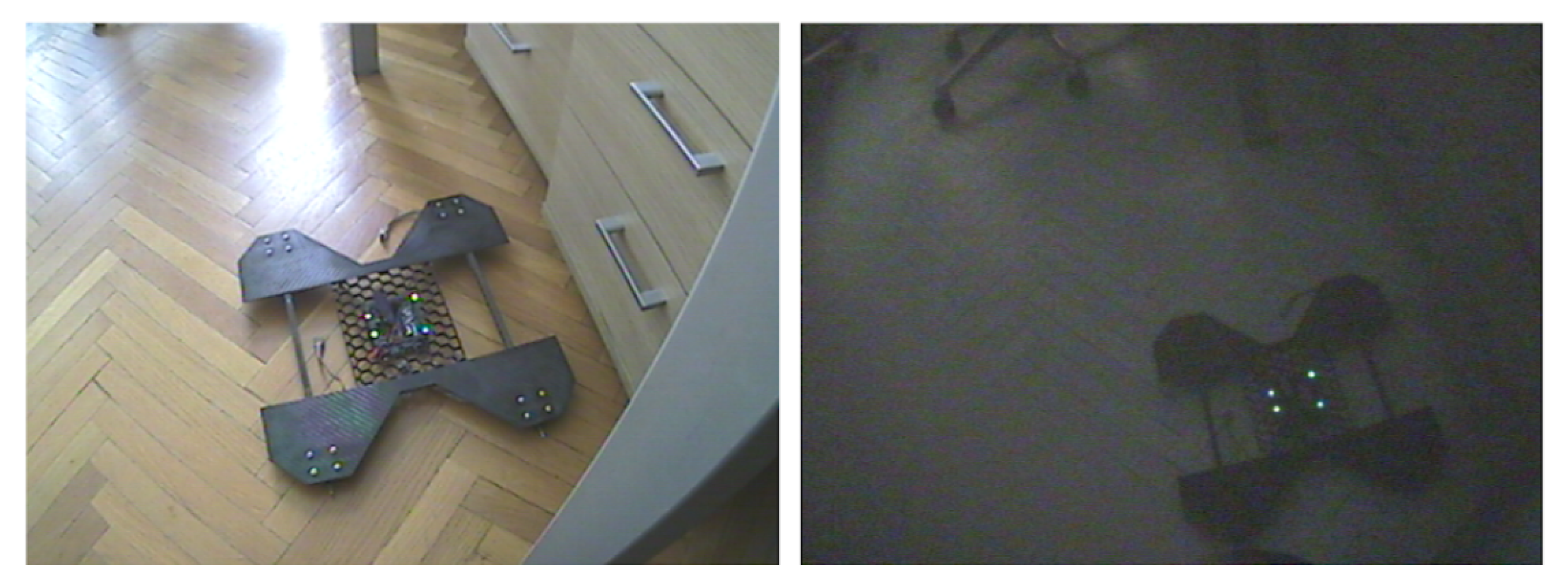
The redesign of the aMussel top cap ties into the change of the visual sensor used by the aPad. The original aPad vision system consisted of four splash-proof analog outdoor cameras mounted to look over each docking mechanism, with layers of infrared filtering film applied until only the bright output of the IR LEDs on the aMussels was visible even in daylight (Figure 5).

This was changed to a single Microsoft Kinect IR and RGB combination sensor encased in a watertight plexiglass tube, mounted on a specially designed motorized pan mechanism which allows it to turn and look down over each of the four docking mechanisms (Figure 6). Thus, the mechanical turning of the sensor replaced the switching between four separate camera sources, and the Kinect’s IR emitter replaced the IR LEDs on the aMussel, achieving both image quality improvement and increased range, better system longevity, and overall simplification of the vision system implementation. The camera is mounted sideways to maximize its vertical field of view, since it achieves a full 360 horizontal field of view by rotating using the pan mechanism. A sun protection sticker was applied to the plexiglass tube to prevent the sensor overheating during prolonged deployment and operation in direct sunlight. The platform’s GPS antenna is additionally mounted on top of the tube to ensure the best signal reception possible.

2.1.3. aPad Docking Unit

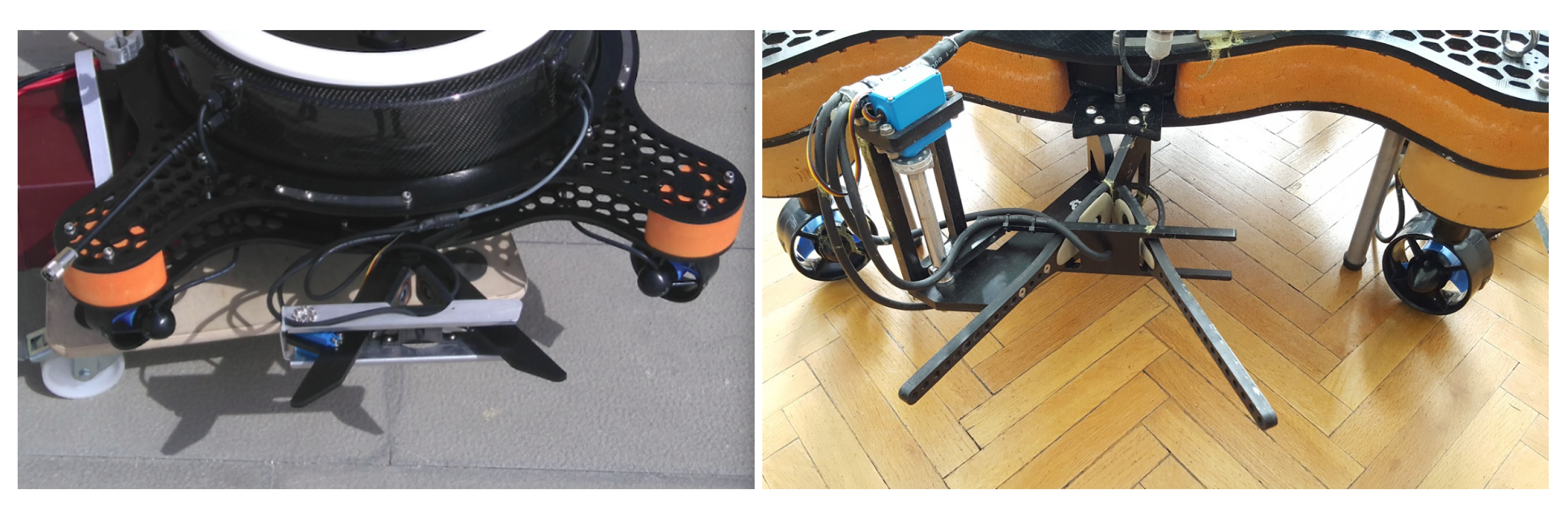
Each of the four charging docks on the aPad contain three charging coils encapsulated in waterproof resin which provide wireless energy transfer to the corresponding coils on an aMussel top cap. The mechanism consists of two immovable delrin levers which act as a guiding rail funneling the aMussel towards the charging dock, while a motorized shutter pushes on the aMussel while closing, mechanically locking the aMussel into position once slotted. To be able to operate in real-world conditions, the docking mechanism is designed to have high tolerances to offsets with regards to the approaching aMussel, including vertical shift tolerance of ±50 mm, and horizontal shift tolerance of ±130 mm.

After several field and stress tests, the docking mechanism was modified to keep the servo motor moving the arm well above water (as its water resistance rating proved not high enough to tolerate repeated complete submersion). This also reduced the force it needed to exert during closing by ensuring better leverage, thus avoiding excess mechanical wear and increasing the longevity of the motor as well as the entire mechanical system. The design of the dock itself was modified and streamlined by thinning and lengthening its two prongs for more horizontal tolerance during docking (increased to ±180 mm), as can be seen in Figure 7.

2.2. Docking Algorithm

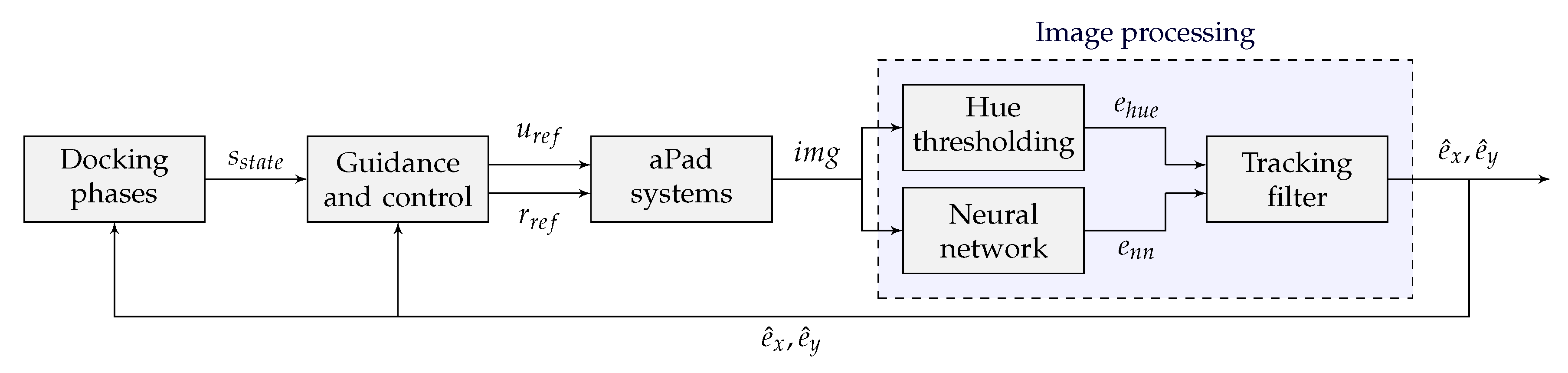
The docking algorithm described in this paper is realized using several components. The general control structure is shown in Figure 8. Docking phases implement a state machine which represents the highest level of control within the algorithm. Its output $s_{state}$ represents the current state the system is in. Guidance and control algorithms generate references for low-level speed controllers in active use by the aPad’s on-board systems with $u_{ref}$ being the surge reference and $r_{ref}$ being the yaw reference, while Image processing takes the image $img$ acquired from the aPad’s camera and employs traditional computer vision methods to output the aMussel image position estimate $e_{hue}$ and neural network object detection to produce the image position estimate $e_{nn}$, then fusing them using a filtering node featuring an Extended Kalman Filter, in order to provide visual feedback. The final outputs of the filter node are ${\widehat{e}}_x$ and ${\widehat{e}}_y$, representing the estimates of the horizontal and vertical image coordinate of the aMussel, respectively.

In [28], the authors detail the dynamic and kinematic models of the aPad over-actuated surface platform and several of its control structures. This subsection discusses the aspects strictly related to achieving autonomous docking capabilities within the swarm.

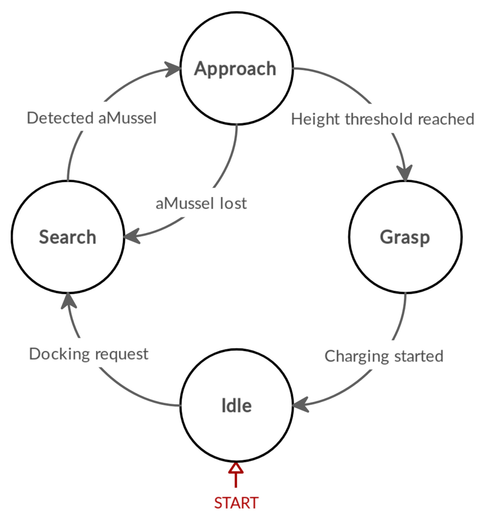
Figure 9 shows the aPad docking algorithm represented as a state machine. While docking, the aPad goes through three active states. An Idle state is also present to account for the times when the aPad is holding its position as the docked aMussels charge and transmit data.

• Search: The aPad rotates at a set rate until it registers a camera frame in which the top cap of an aMussel is visible.
• Approach: The aPad moves towards the detected aMussel, regulating its yaw and surge speeds in tandem, turning to keep it centered in its camera field of view. Should the aMussel be lost from view for a preset number of frames during this phase, the aPad will recommence Search.
• Grasp: The aPad closes the servo-actuated gripper on its docking mechanism once the reported position of the aMussel is below a set height threshold. Wireless charging is started.

Before each docking attempt starts (launching into the Search state), the pan mechanism rotates the Kinect sensor to face the chosen dock by giving it one of four preset positions. To compensate for any drift or other mechanical offsets accrued during the aPad’s operation, after the initial rotation towards the selected dock, the pan movement will be subject to additional small adjustments if the dock is not completely centered in the current camera image. This is accomplished by applying a simple feature-matching algorithm based on Fast Library for Approximate Nearest Neighbors (FLANN) with Scale Invariant Feature Transform (SIFT) descriptors to the image, making use of the dock’s very recognizable and known fixed features (mechanism prongs, servo motor housing) as a template.

During the Approach phase, the servo-powered docking mechanism arm will close once the estimated image height of the located aMussel top cap falls below a vertical threshold, indicating that the agent has come close to the camera as well as the docking mechanism slot that the camera is pointing towards. 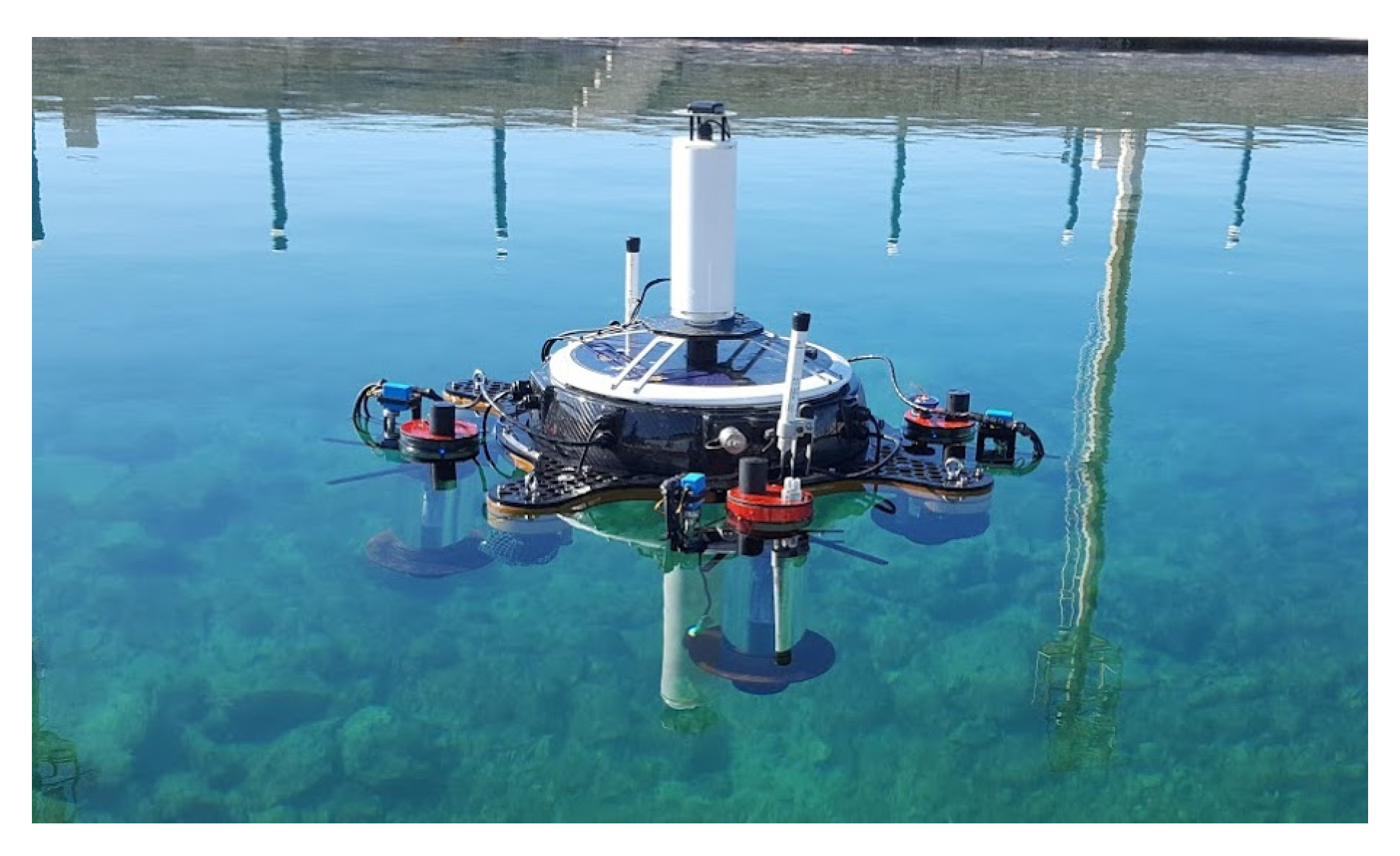This height threshold is a preset value that is calibrated with regards to the camera tilt angle and the buoyancy and floating height of an aMussel that has completely surfaced, and was set to $25\%$ of the full image height for the experiments described in this paper. The aPad will consider the correct agent docked once it notes a rising edge in the charging status of the aMussel that was the docking target. If the mechanism closing was triggered but the aMussel is not charging, i.e., it has not been properly docked, the aPad will retry the docking procedure. An example of the final docking outcome, an aPad with four successfully docked aMussels, is given in Figure 10.

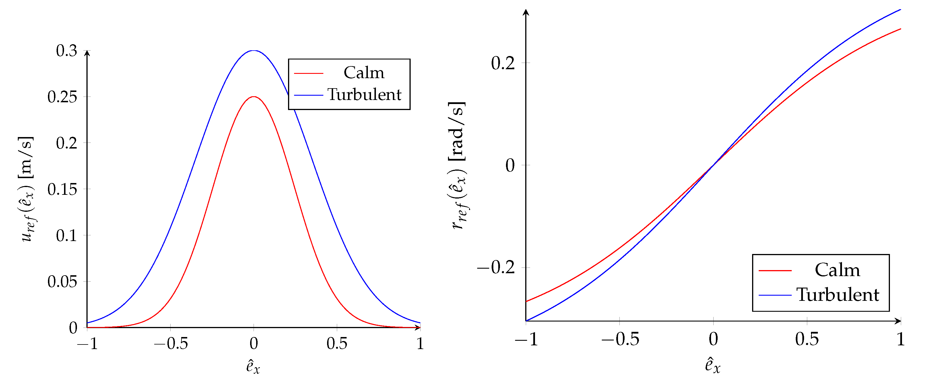
The curve given in Figure 11, left, represents the surge speed regulation of the aPad. The closer the estimated final image position of the aMussel is to the center of the image and thus the better aligned it is with the dock, the faster the aPad will approach it. The curve in Figure 11, right, represents the yaw rate regulation of the aPad, with the goal of keeping the aMussel top cap aligned with the aPad’s docking mechanism.

Surge speed control references are generated using:

$$u_{ref}\left({\widehat{e}}_x\right)=k_1{e}^{-\frac{{\widehat{e}}_x^2}{2{\sigma }^2}}$$

(1)

and those for yaw rate control are done using:

$$r_{ref}\left({\widehat{e}}_x\right)=k_{2}tanh\left(a{\widehat{e}}_x\right)$$

(2)

where the input ${\widehat{e}}_x$ represents the estimate of the horizontal image coordinate of the aMussel scaled to an interval of [−1, 1], received from the filter node. A fixed yaw rate $r_{ref,search}$ is set for the search phase of the docking process. In the process of the experimental validation of the system, the decision was made to include two sets of parameters depending on the conditions the docking was to take place in, discussed in more detail in Section 3. Values chosen for regulator parameters for working in calm water conditions and for working in a more turbulent environment are given in

Table 1. Regulator parameters.

Parameter	Value-Calm	Value-Turbulent
$k_1$ [m/s]	0.25	0.3
$k_2$ [rad/s]	0.35	0.4
$\sigma$	0.245	0.35
a	1	1
$r_{ref,search}$ [rad/s]	0.3	0.4

.

Depending on which of the four aPad docks the aMussel is being docked to (or undocked from), the surge reference needs further transformation. A rotation matrix is applied to the generated surge reference from (1):

$${{\mathit{u}}^{\prime }}_{ref}=\left[\begin{array}{c}{u}_{ref,x}^{\prime }\\ u_{ref,y}^{\prime }\end{array}\right]=\left[\begin{array}{cc}cos\left(\alpha \right)& -sin\left(\alpha \right)\\ sin\left(\alpha \right)& cos\left(\alpha \right)\end{array}\right]{\mathit{u}}_{ref,0}$$

(3)

where $u_{ref,0}$ represents the reference for the default front-facing dock which is used to determine the vehicle’s heading:

$${\mathit{u}}_{ref,0}=\left[\begin{array}{c}{u}_{ref}\\ 0\end{array}\right]$$

(4)

Angle $\alpha$ is simply determined using $\alpha =i_{dock}\frac{\pi }{2}$, with $i_{dock}$ as the index of the chosen dock, as shown in Figure 12.

For undocking an aMussel, the aPad opens the corresponding dock and moves “backwards” using the negative of the calculated surge reference for a fixed period of 10 s. This ensures the aMussel in question exits the dock and is clear of the aPad.

Implementation-wise, the complete aPad operating system and software components run on an Intel NUC i5 mini PC situated within its round hull. Lower-level controllers such as the described yaw and surge controllers, thruster allocation, sensor drivers including the Microsoft Kinect and related image processing utilities, as well as navigation and tracking filters are implemented in C++ and organized in packages, services, and executable nodes under the Robot Operating System (ROS) middleware paradigm. Higher-level control also realized in ROS includes mission primitives making use of dynamic positioning, line following and go-to-point controllers, as well as the here relevant docking mission primitive implementing the phases shown in Figure 9. At the top of the hierarchical code structure, an Application Programming Interface (API) written in Python was developed to enable simple high-level mission planning and execution. The missions carried out during field experiments described in Section 3 were all realized using this API. More details and additional features of the software architecture can be found in [27].

2.3. Image Processing

Achieving a good degree of accuracy in image processing—especially when it is used as one of the main methods of robot perception—is key in real-world applications. The image processing approaches used for locating the aMussel and correctly navigating towards it evolved through several stages that roughly correspond to the evolution of the system hardware. These include IR-only intensity thresholding, hue-based thresholding, and neural network detection.

Taking into account the evolution of the system, the ability to switch between (“legacy”) IR mode and the more recent full RGB image modes is of practical significance, as this duality and the capability of the Kinect sensor to switch between infrared and regular camera means swarm work in dark or night-time conditions can still proceed, if necessary. The IR-only intensity thresholding approach to visual servoing was described in detail in [4] and used as the main method during indoor testing of the system and the initial docking experiments described in the paper. This section focuses on the implementation of the two primary image processing variants making use of the RGB camera mode.

Please note that although the Kinect sensor is mounted sideways, all images are processed without rotation. Rotation is done later in coordinate calculations before feeding information to the parts of the system which formulate aPad movement references, which saves time in potentially costly image processing operations. For ease of viewing and reading, the images presented as examples in this paper have been rotated.

2.3.1. Hue-Based Thresholding

The original implementation of the hue-based thresholding method for detecting and locating aMussels in an image are described in [2,4]. This subsection describes the final implementation used in the subCULTron system.

The RGB image received from the Kinect sensor is first cropped to a region of interest representing a fixed distance in front of the camera in which an aMussel might realistically be located. This serves to both minimize the chances of false-positive detections and not waste processing time on a region of the image that is likely to contain only sky. Currently the crop disregards the upper 25% of the 640 pixels high image. The cropped image is then converted into the HSV (Hue Saturation Value) color space, and Contrast-limited Adaptive Histogram Equalization (CLAHE) is applied to it in the interest of minimizing the effects of varying lighting conditions (for examples of using CLAHE to improve visibility in noisy conditions and poor lighting, see [29,30]). Finally, a threshold based on hue values for the color red is applied to the image. After thresholding, a bounding box is placed around the largest detected blob of pixels remaining in the image. The coordinates of the bounding box are the input of the visual servoing controller. The origin of the coordinate system is in the center of the image, and for control purposes all coordinates are scaled to a range of [−1, 1], with [−1, −1] representing the left-hand bottom corner, and [1, 1] the right-hand top. Figure 13 shows two examples of aMussel top caps detected in the RGB camera image.

Several heuristics to improve detection have been implemented. There is a minimum blob size requirement for detection to remove noisy false-positive detections of reflections, floating debris or similar. Primarily, the size of the pixel blob and its position in the image are considered: for example, if a very large blob is positioned higher in the image, it is highly unlikely to be an aMussel, and will be disregarded.

As noted in [4] and included here briefly for completion and relevant comparison, an analysis of image data collected on-site and processed with the developed hue-based aMussel detection algorithm was compared to manually annotated data in order to achieve a benchmark. The results are shown in

Table 2. Comparison of frame counts with and without aMussels present.

Manually annotated data	No mussel	1723
	Mussel present	1098
Automatically processed data	No mussel	1847
	Mussel present	974

and

Table 3. Frame count breakdown for aMussel detection algorithm.

Correctly detected empty frames	1700
False-positive frames	23
Missed frames	147
Correctly detected non-empty frames	951
Total frames processed	2821
Success rate	86.61202%

.

2.3.2. Neural Networks for Object Detection

The decision to use artificial neural networks trained for object detection and recognition was made in an attempt to improve the aMussel detector beyond the above outlined abilities and limitations of the hue-based thresholding. The goal was making it more universal, less reliant on lighting conditions and thus needing fewer hue threshold adjustments before deployment, as well as to increase maximum detection distance and generally increase robustness.

The neural network training was done on a PC with two Nvidia GTX 1080 Ti graphical processing units, running the Nvidia CUDA toolkit to achieve parallel computing. The training process was further sped up using the OpenCL framework which enabled the learning to also be executed on the CPU—in this case an Intel Core i9 9900k with 8 cores and 16 threads running at frequencies up to 5 GHz.

A dataset consisting of 3105 images containing an aMussel was constructed from a mixture of data collected in several locations and under varying conditions at Jarun lake in Zagreb, Croatia, the seaside at Biograd na Moru, Croatia, and the Arsenale and lagoon of Venice, Italy. Object detection and recognition networks were trained with one detection class in mind—the $amussel$ class, using the Tensorflow library [31]. Dataset annotation in the form of labeled bounding boxes was done manually using the open source LabelImg tool [32].

Several popular object recognition models were trained and tested, in the interest of finding the best one for the specific application. The selected models are the Single Shot Detector with MobileNet version 2 (SSD MobileNetV2) [33] trained in two instances for two different input image sizes (a small and fast 300 × 300 resized version, and a 480 × 480 version without resizing), and the Fast Region-based Convolutional Network method (FR-CNN) [34]. Additionally, a You Only Look Once version 3 detector (YOLOv3) was trained on the data using its own specific training pipeline [35]. 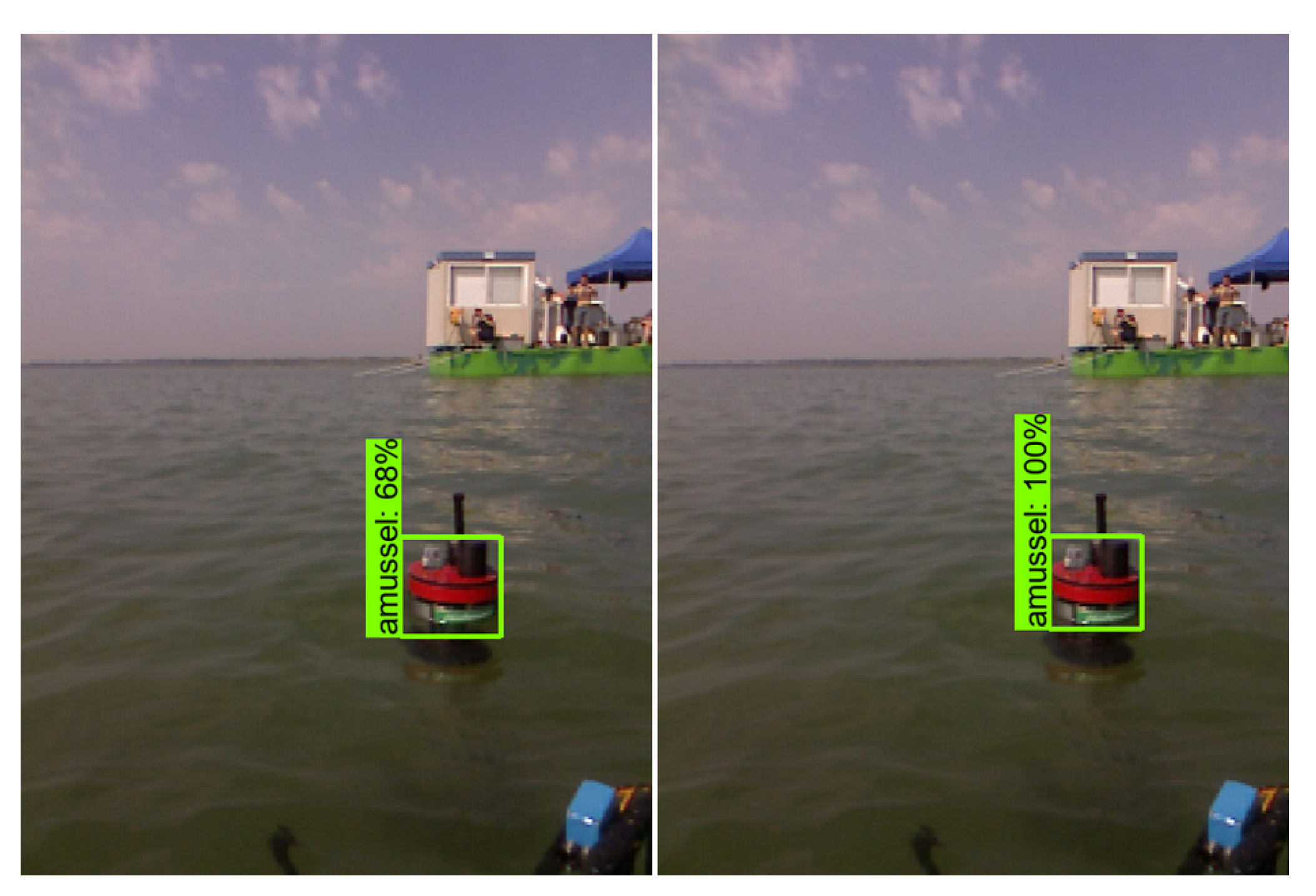An example comparison of the neural network output compared to the labeled “ground truth” it is learning from can be seen in Figure 14.

On the dataset of 3105 images, a 90/10 train/test split was used, and validation was later additionally run on an entirely fresh unseen dataset. Testing the final frozen graphs on both train and test data yielded only a marginal decrease of accuracy on the previously unseen test-exclusive split of the dataset, implying that no significant overtraining occurred and the networks were appropriate for further testing and use. 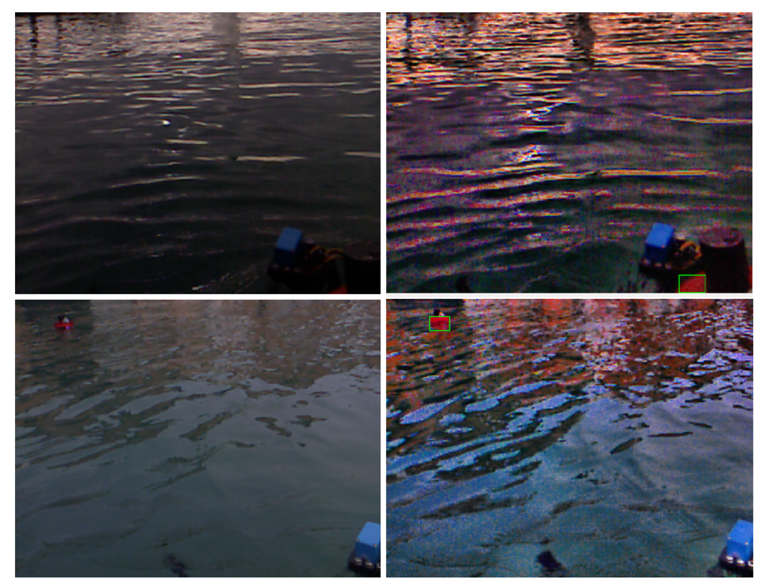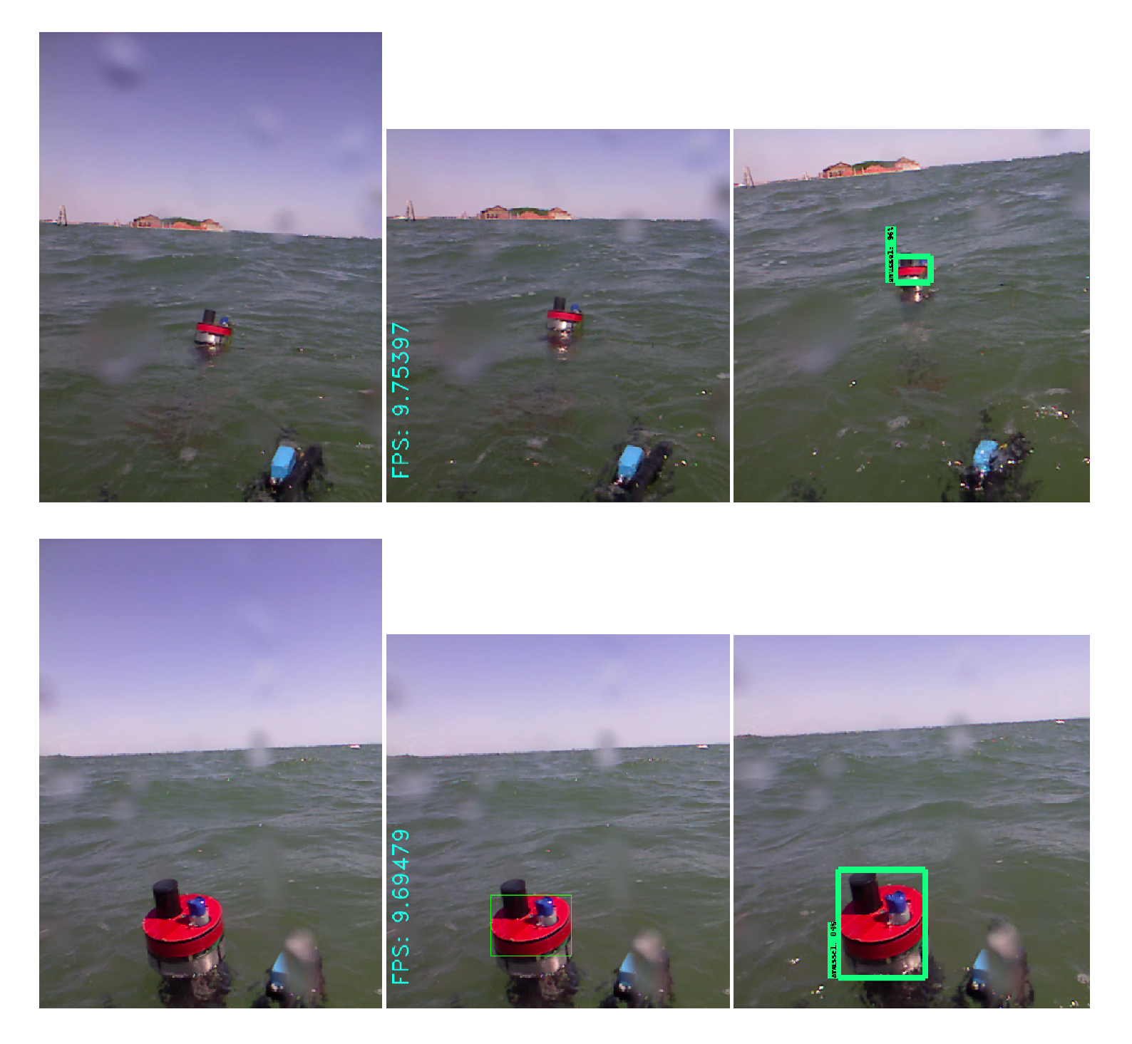Some examples of detection in challenging circumstances that neural networks were helpful in resolving are shown in Figure 15—including cases with larger distances from the camera, partial visibility, occlusion, wave splashes/partial submersion, bad lighting and weather conditions, and sunlight glare.

Striking a balance between detection reliability and framerate on the limited computer running within the aPad was a significant part of the task. Framerates were tested on the Intel NUC i5 on-board computer on the marine platform, running in parallel with the control structures of the aPad, as these are the operating conditions relevant to the application. Performance results are shown in

Table 4. Comparison of mean average precision in single-class object detection and single image frame processing time on on-board computer (bold is best, italic is final choice).

Model	mAP	Seconds Per Frame (Average)
SSD Mobilenet v2 300 × 300	0.6452	0.1
SSD Mobilenet v2 480 × 480	0.7064	0.2
Faster R-CNN	0.7375	1.6
YOLOv3	0.9352	2.7

, where mean average precision (commonly known as mAP) was used as a measure of model reliability and object detection quality [36].

YOLOv3 offered excellent accuracy, but was computationally demanding (especially since there is no dedicated GPU present on the aPad) and thus too slow when running in real time. After testing and benchmarking, as the best compromise between detection quality and reliability and framerate, the SSDN MobileNet V2 with no additional image resizing was chosen, but a ROI crop was applied to the input image, same as in the hue thresholding method.

Running in parallel, the original hue thresholding algorithm is capable of outputting processed images at a rate of 10 FPS, meaning the neural network will be made to process only the latest image it has in its input queue, potentially skipping some older enqueued image frames in order to not lag behind significantly enough to affect the docking process. The outputs of the hue thresholding and the neural network detection are then fused together to determine the final aMussel position estimate, as will be shown in the following section.

2.4. Tracking Filter

To combine the output of the classical hue thresholding approach (which had proven quite reliable in close quarters) and the neural network approach to image processing, an extended Kalman filter (EKF) was introduced into the system. The node containing the filter operates in the image coordinate space, and fuses together aMussel position measurements. It also acts as a tracking filter, using previously acquired information about the speed of the aMussel’s movement in the image to ensure more accurate state predictions.

The filter operates at a fixed rate of 10 Hz, so a time step of $\Delta t=0.1$ s is used in all internal calculations.

The state vector of the filter is given with

$$\mathbf{x}={\left[\begin{array}{cccc}{\widehat{e}}_x& {\widehat{e}}_y& v_x& v_y\end{array}\right]}^T$$

(5)

where $v_x$ and $v_y$ are velocities derived from the difference of the last two estimated states, and ${\widehat{e}}_x$ and ${\widehat{e}}_y$ are position estimates based on measurements fused from the two sources. The state model used can be expressed with $\dot{\widehat{\mathbf{e}}}={\left[\begin{array}{cccc}{v}_x& v_y& 0& 0\end{array}\right]}^T$.

The measurement vector of the filter is given with

$$\mathbf{y}={\left[\begin{array}{cc}{e}_x& e_y\end{array}\right]}^T+{\left[\begin{array}{cc}{r}_x& r_y\end{array}\right]}^T$$

(6)

where $e_x$ and $e_y$ represent $(x,y)$ image coordinate pairs calculated using measurement fusion and scaled from pixel values to a [−1, 1] range.

Results received from the two measurement sources are represented with ${\mathbf{e}}_{\mathbf{nn}}={\left[\begin{array}{cc}{e}_{nn,x}& e_{nn,y}\end{array}\right]}^T$ containing the results of neural net processing and ${\mathbf{e}}_{\mathbf{hue}}={\left[\begin{array}{cc}{e}_{hue,x}& e_{hue,y}\end{array}\right]}^T$ containing the results of hue-based image thresholding.

Meanwhile, $r_x$ and $r_y$ are the respective measurement variances used to take into account measurement quality and reliability along each axis. These are defined as:

$$r_x\sim \mathcal{N}(0,{\zeta }_x)$$

(7)

$$r_y\sim \mathcal{N}(0,{\zeta }_y)$$

(8)

The values of ${\zeta }_x$ and ${\zeta }_y$ are determined using values for each measurement source, ${\zeta }_{\mathbf{nn}}={\left[\begin{array}{cc}{\zeta }_{nn,x}& {\zeta }_{nn,y}\end{array}\right]}^T$ for neural net processing and ${\zeta }_{\mathbf{hue}}={\left[\begin{array}{cc}{\zeta }_{hue,x}& {\zeta }_{hue,y}\end{array}\right]}^T$ for hue-based image thresholding.

For neural network data, the values of ${\mathbf{\zeta }}_{\mathit{nn}}$ are set to an empirically determined constant:

$${\zeta }_{nn,x}={\zeta }_{nn,y}=0.075$$

(9)

However, for the hue thresholded data, the ${\mathbf{\zeta }}_{\mathbf{hue}}$ values were defined as depending on the vertical position of the detected pixel blob in the image. The further away on the y-axis the detected blob is, the higher the variance of the hue-based detector, i.e., hue-based detection is less trusted. It is set with:

$${\zeta }_{hue,x}={\zeta }_{hue,y}=\frac{1-e_{hue,y}+0.2}{2}$$

(10)

Considering the image y-coordinate ranges from −1 at the bottom of the image, and 1 at the top, the variance values used in the filter achieve a range of [0.1, 1.1], which is always higher than any concurrently available neural network detector value.

Thus, using methods explained in [37,38], the fusion of measurements from two sources is done with:

$$e_x=\frac{{\zeta }_{hue,x}{e}_{nn,x}+{\zeta }_{nn,x}{e}_{hue,x}}{{\zeta }_{hue,x}+{\zeta }_{nn,x}}$$

(11)

$$e_y=\frac{{\zeta }_{hue,y}{e}_{nn,y}+{\zeta }_{nn,y}{e}_{hue,y}}{{\zeta }_{hue,y}+{\zeta }_{nn,y}}$$

(12)

$${\zeta }_x=\frac{{\zeta }_{hue,x}{\zeta }_{nn,x}}{{\zeta }_{hue,x}+{\zeta }_{nn,x}}$$

(13)

$${\zeta }_y=\frac{{\zeta }_{hue,y}{\zeta }_{nn,y}}{{\zeta }_{hue,y}+{\zeta }_{nn,y}}$$

(14)

Implementation-wise, three distinct cases exist. If hue-based detection has produced a result, but no detection data has been received from the neural net, ${\mathbf{\zeta }}_{\mathit{nn}}$ values will both become zero, while ${\mathbf{\zeta }}_{\mathit{hue}}$ will be calculated using (10). The fused measurements $e_x$ and $e_y$ will simply become $e_{hue,x}$ and $e_{hue,y}$, respectively, while ${\zeta }_x$ and ${\zeta }_y$ will become ${\zeta }_{hue,x}$ and ${\zeta }_{hue,y}$.

Likewise, if no detection data has been received from the hue processing node while a valid result has been given by the neural net, ${\mathbf{\zeta }}_{\mathit{hue}}$ will be a zero-vector and ${\mathbf{\zeta }}_{\mathit{nn}}$ will be calculated using (9), with the fused measurements $e_x$ and $e_y$ respectively becoming $e_{nn,x}$ and $e_{nn,y}$, and ${\zeta }_x$ and ${\zeta }_y$ becoming ${\zeta }_{nn,x}$ and ${\zeta }_{nn,y}$.

Finally, if both nodes have sent valid object detection data, their respective variances and fused measurements are calculated as has been described above in (9)–(14).

In addition to distance-based variance calculation, the filter node contains several heuristics aimed at improving data fusion and detector behavior:

• Kinect pan movement flagging. The filter will not take into account measurements acquired while the Kinect sensor was actively rotating, and will only react once a valid docking mechanism-aligned position has been reached.
• Region of interest crop. As the filter converges, any filter outputs outside of the designated realistic “region of interest” (−1 to 1) are discarded.
• Continuous detection requirement. The filter will only output fused measurements after a preset number of consecutive frames have been determined to contain an aMussel, by any of the two detectors. This acts as a sort of outlier rejection for brief usually single-frame false-positive detections.
• Measurement discontinuation detection. If more than 3 s have passed without fresh measurements from either detector, the filter will stop feeding measurements into the docking controller, and the filter will be flushed and reinitialized. This ensures no action is taken based on outdated information. If the aPad was approaching an aMussel and lost it from view this long, as per the previously described state machine the docking algorithm will return to the Search state.

3. Results and Discussion

The subCULTron swarm has in the four years of the project’s runtime been through many tests and demonstrations, including numerous field deployments and experimental trials. The docking segment in its various incarnations has been included and tested throughout. Previous work can be found in [4] in which the initial indoor experiments which served as proof of concept for the wireless charging are described, as well as some initial outdoor experiments aimed at testing the capabilities of the aMussel and aPad positioning systems.

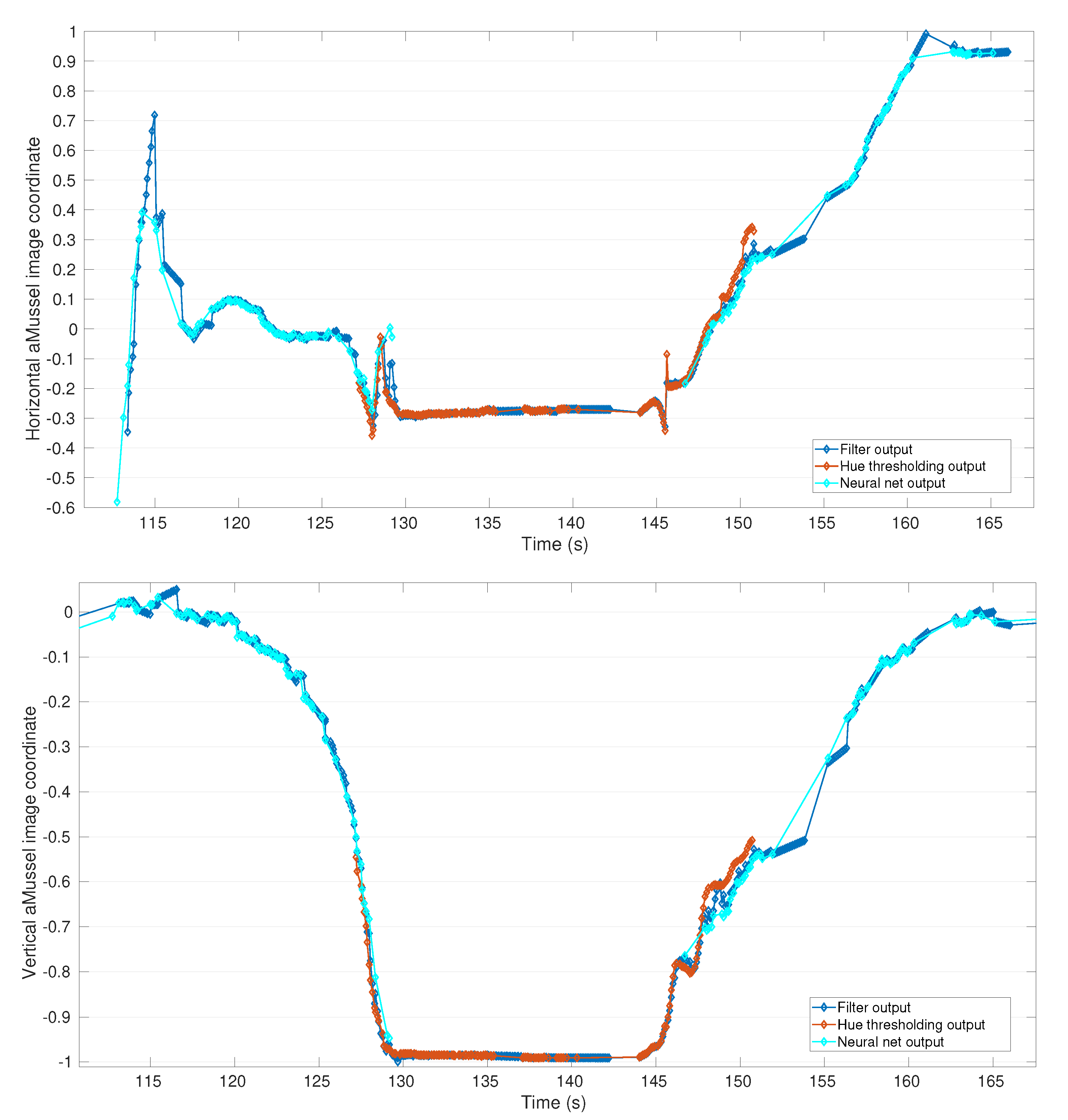
For a closer look at and discussion of the outputs of the image processing and filtering nodes, Figure 16 shows a comparison of the hue thresholding result, the neural network result, and the final filter output during a single successful docking attempt performed in the sea of Biograd na Moru, Croatia. Docking occurs around the 130 s mark, and undocking around 145 s. This sample collection of outputs clearly demonstrates the expected behavior of the image processing system as a whole, as the neural network successfully performs the initial agent detection over longer distances, after which hue thresholding comes into play as the aMussel approaches the camera, ultimately taking over as the aMussel enters the dock, with the filter seamlessly segueing between the two sources. Neural net measurements are largely not present while the aMussel is tightly held within the dock, as the robot is mostly out of the camera’s field of view. However, hue thresholding output persists, as small segments of the red top cap remain visible.

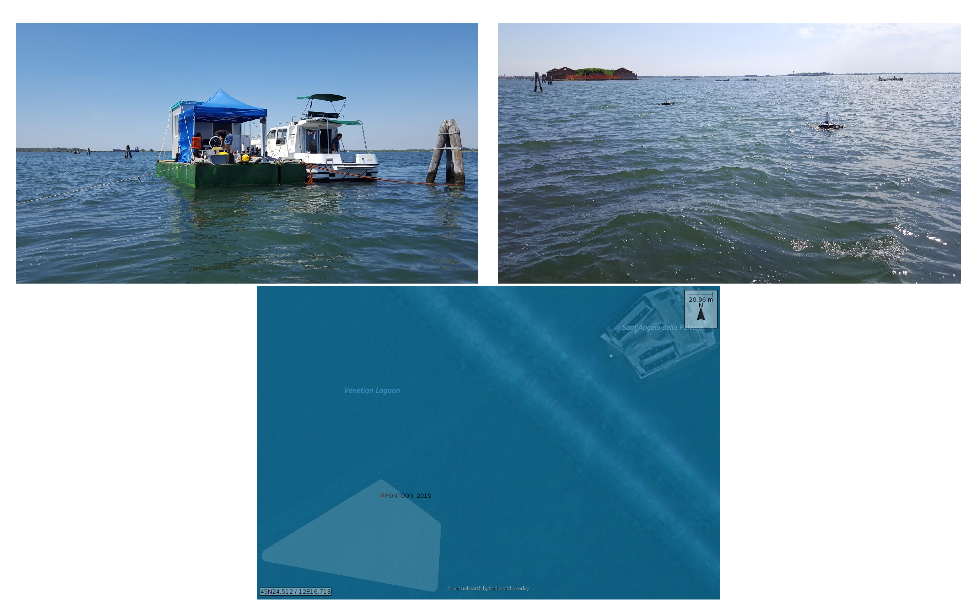
Presented in the rest of this section is a detailed writeup of two particular experiments: a structured experiment to determine the capability of and validate the final docking procedure undertaken at lake Jarun in Zagreb, Croatia; and a “stress test” in a challenging environment on-site near the island of Sant’Angelo della Polvere in the lagoon of Venice, Italy.

3.1. Structured Docking Experiment

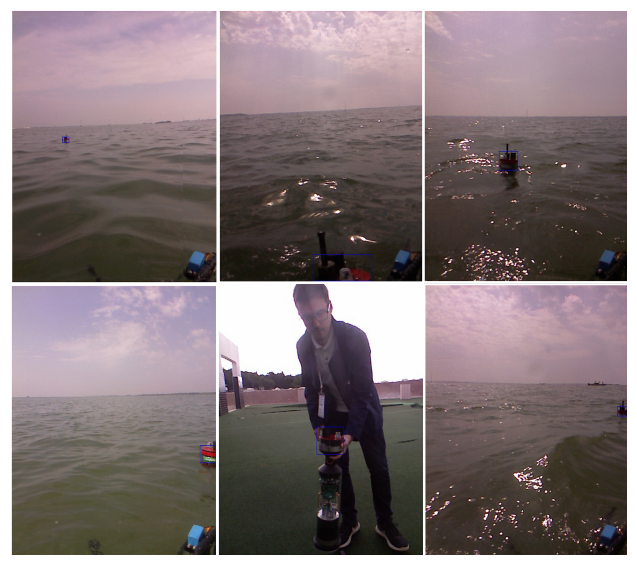
The structured docking experiment took place in June 2019, with the goal of validating the final developed system. The experiment location and a shot of the experiment in progress can be seen in Figure 17.

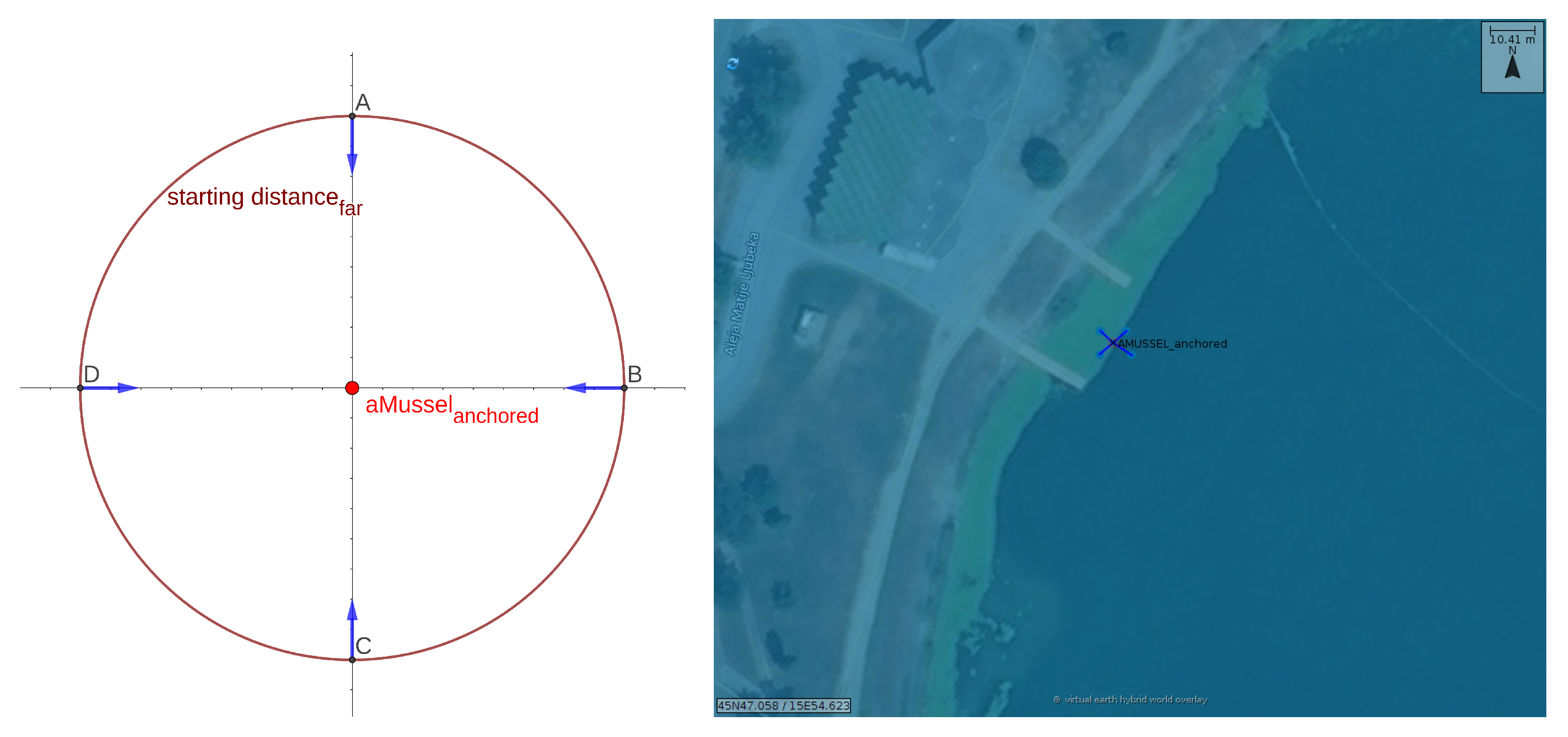
To test the docking algorithm in a controlled and verifiable setup, an aMussel was anchored using rope and metal weights and its position was recorded using the aPad’s GPS with Real-time kinematic (RTK) positioning technique capabilities for maximum accuracy. This measurement was then used as a ground truth reference for aMussel position throughout the experiment and provided information about position offsets and distances of the aPad from its goal.

After setting up the anchored aMussel, four primary aPad starting positions were chosen along a circle with a radius corresponding to an empirically established maximum distance of consistently reliable docking. This maximum distance was determined to be between 4 and 5 meters of distance from the aMussel—note that docking from further away is possible (with “lucky” cases of successes from as much as 15 meters away), but is not necessarily consistent and thus not considered reliable or suitable for an autonomous system. The starting positions were then distributed along the circle as seen in Figure 18, so that the four major approach directions were included, in order for the effects of sunlight and glare to be accounted for during the experiment. Please note that during the final run of the experiment presented here, it was run twice from the direction of the first starting point and thus five docking attempts are shown. The Neptus C4I Framework was used for aPad mission supervision and control [39]. The starting point to anchor point distances reported by Neptus were, starting from the northernmost point and continuing clockwise: 4.18 m, 5.11 m, 4.13 m, and 4.16 m.

The aPad would be manually sent to each of the marked starting points and turned so the aMussel was not immediately in view, after which the docking algorithm would be started. After each successful docking, the aMussel would be released and the aPad sent to the next point. The experiment was concluded once a continuous run of docking attempts from all directions was achieved.

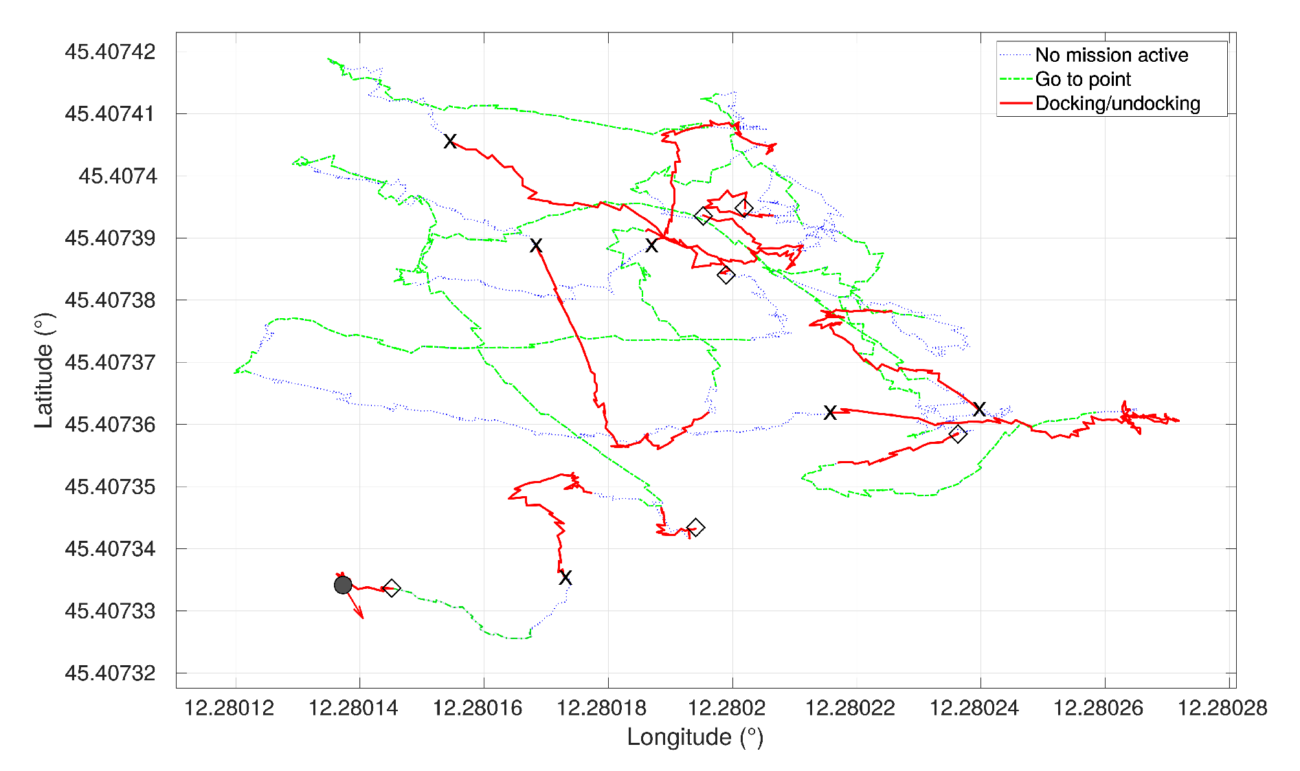
Figure 19 presents the trajectory of the aPad during the experiment, with denoted color-coded segments during which each of the mission primitives (docking/undocking, going to next point, and no mission selected) were active.

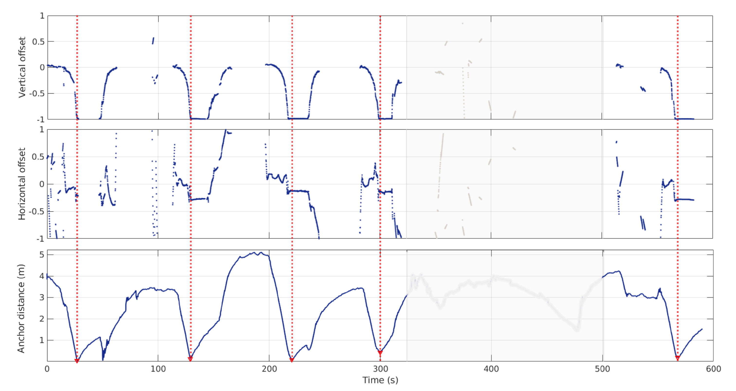
During the experiment, horizontal, vertical, and total offset data was recorded. The horizontal and vertical offsets refer to the position of the aMussel relative to the center of the image frame, as output by the EKF. The aMussel total offset refers to the calculated distance between the current position of the aPad and the saved position of the anchored aMussel. These are all shown in Figure 20, where the five docking attempts are all evident: the distance from the aMussel decreases, and it simultaneously moves towards the bottom of the image while being kept horizontally centered.

Please note that for about three minutes between the fourth and fifth docking attempt the aPad was not actively performing the docking experiment, but rather having minor maintenance performed and entangled lily pads and debris removed from its hull and docks. This data was left included for consistency as it was recorded during the experiment, but it has been grayed out in plots as it is not relevant or informative.

During the fifth docking attempt shown (starting at 510 s on the graphs in Figure 20) it can be seen how the aPad briefly loses sight of the aMussel, returning to the Search state, then finds it once again after some rotation, continuing and concluding the docking attempt successfully.

The anchoring of the aMussel and the aPad’s position estimate are both imperfect, and continued docking attempts nudged the anchor slightly from its original noted position, so the distance between the aPad and the aMussel can be seen approaching zero but still with a slight offset. Due to the length of the rope used for anchoring, the aPad also had some leeway to move with the aMussel while holding it docked, but upon release the aMussel moved back towards its original position—hence the small rise and fall in distance just after each docking concluded.

The jagged quality of the lines representing the trajectory of the aPad during the experiment and the small jumps in position are a result of the aPad’s navigation filter updating with GPS measurement corrections received in fixed time intervals.

The previously described implemented filter heuristics turned out to be very helpful in dealing with brief flashes of false-positive detections, eliminating problematic reaction to them all but entirely. The aPad was able to successfully dock the aMussel from each direction, and was able to resume and successfully conclude a docking attempt after losing sight of its target.

3.2. Challenging Environment Test

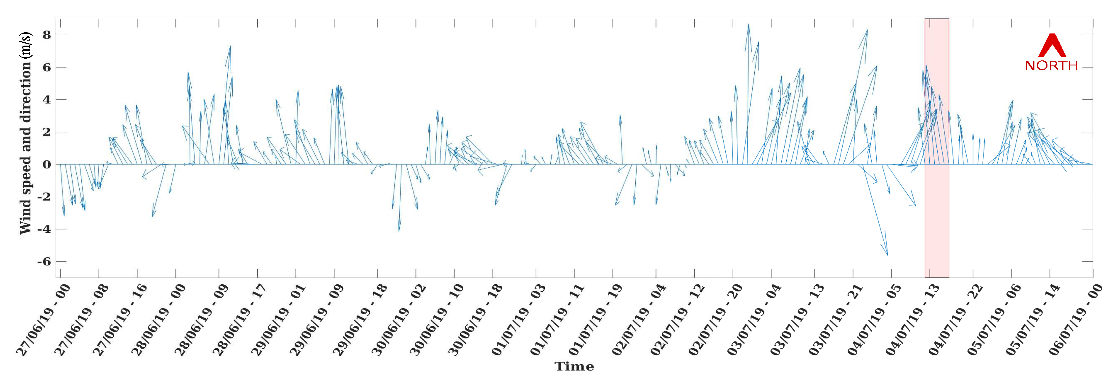
The realistic environment docking experiment took place during a prolonged set of field trials for the subCULTron project in July 2019, on a particularly windy day with rough, choppy waves making for challenging conditions but providing a good opportunity to test the operational limits of the docking system (see Figure 21).

The subCULTron robots were deployed off a pontoon, with a designated open sea workspace next to a relatively low-traffic water route (Figure 22). Unlike the structured experiment, no data about the aMussel’s position was available. Image-derived data and information about when each of the docking attempts started and concluded were collected.

Figure 23 presents the full trajectory of the aPad during the experiment, with color-coded segments showing when each of the mission primitives were active and markers showing the moment of each docking and undocking. The aMussel was drifting in currents of varying strengths towards the northwest of the given image, leading to noticeable differences in position between where the aPad leaves it after undocking and where it is later caught (i.e., the black markers on the trajectory plot). A video including visual feeds from the Kinect, image processing and EKF data, and a mission replay constructed from the aPad mission data logs for the autonomous docking field experiment can be seen at https://www.youtube.com/watch?v=Agky3vv6Mh4.

Figure 24 gives a full timeline of the image offsets detected by the hue thresholding and the neural network, as well as the final filter output for the sequence of six successful docking and undocking attempts. Both docking attempts and undockings can be clearly seen, as the offsets reflect how the aPad approaches the target and captures it, then, after holding it for a while, releases it and moves away. This corresponds to the previously discussed results shown in Figure 16. Please note that the filter node was only running during docking attempts, so there are no filter output data points between the conclusion of each attempt and the start of the next one.

As briefly noted in Section 2.2, experiments in real conditions in the lagoon led to a tuned increase in all regulator parameters, as the ones previously used made for an aMussel-catching approach that, while successful, was very slow and tentative in the presence of waves and wind and sea currents. To accommodate the aMussel bobbing up and down on the waves and briefly being lost from the aPad’s view, the parameter for the tracking filter heuristic that ensures continuous measurements and rejects fleeting outlier detections was set to only require 3 consecutive frames of detection as opposed to the original 6. While here the switch was done manually, to accommodate the need for this level of adaptability, automated switching between “modes” depending on the output of the aPad’s IMU will be implemented.

The experiment in real-world conditions also showed that the mechanical design of the docking system with vertical offset tolerance was sound, as even with waves causing considerable displacement, the aMussel was successfully caught. The plexiglass-encased vision system also proved robust to these conditions, working even with the casing being sprayed and splashed with water as can be seen in Figure 25.

4. Conclusions

The algorithm and implementation proposed in this paper have proven to fit their intended use in the subCULTron heterogeneous robotic swarm quite well, enabling surface platforms to dock smaller floating sensor nodes using a visual servoing approach, successfully starting wireless energy transfer in a variety of testing conditions with very simple changes in parameter tuning. In the future, these changes will be done autonomously, based on the environmental data measured by the vehicles themselves.

Further work will include stress-testing of the wireless charging itself, as well as thorough testing and benchmarking of its efficiency. Although the mechanical design of the aPad docks and the aMussel top caps have so far shown to ensure satisfactory alignment and proximity of the transmitter and receiver coils, full testing of the long-term energy transfer efficiency and reliability remains to be done. The developed system has been used to charge aMussels during field trials; however, this was only done in strictly controlled conditions on land. As an additional aspect of long-term marine operations, the effects of biofouling on the operation of the swarm will be investigated.

The docking system described here was briefly used in the validation of the exploration paradigm described and tested in [3], and it will be combined with both exploration and high-level decision-making and scheduling algorithms described in [27] in order to enable the examination of the cumulative effects of energy transfer systems on the longevity of the subCULTron swarm as a whole, in the interest of maximizing it and ensuring satisfactory, truly autonomous long-term environmental monitoring.