High-Speed Time-Resolved Tomographic Particle Shadow Velocimetry Using Smartphones

Abstract

The video-capabilities of smartphones are rapidly improving both in pixel resolution and frame-rates. Herein we use four smartphones in the “slow-mo” option to perform time-resolved Tomographic Particle Shadow Velocimetry of a vortex ring, using 960 fps. We use background LED-illuminated diffusers, facing each camera, for shadow particle imaging. We discuss in-depth the challenges present in synchronizing the high-speed video capture on the smartphones and steps to overcome these challenges. The resulting 3-D velocity field is compared to an instantaneous, concurrent, high-resolution snapshot with four 4k-video cameras using dual-color to encode two time-steps on a single frame. This proof-of-concept demonstration, supports realistic low-cost alternatives to conventional 3-D experimental systems.

1. Introduction

Since its inception in the early 1980s, particle image velocimetry (PIV) has become the dominant approach to measuring instantaneous velocities in experimental fluid mechanics [1,2]. A typical PIV system consists of at least one camera, a high-intensity light source with accompanying sheet or volume optics, a timing unit, and tracer particles seeded in the flow of interest. Velocity vectors are obtained by measuring the displacement of the particles using a cross-correlation between two images [3]. Using one camera and a light sheet can yield velocities in a single plane known as 2D-2C vectors (two-dimensions, x and y, and two components, u and v). If a second camera is added to make a stereo setup, in and out of plane or w velocities are also measurable yielding 2D-3C vectors. These methods have been further expanded into whole-field, volumetric measurements such as scanning stereo PIV [4], tomographic PIV [5,6] or synthetic aperture PIV [7], which typically use four or more cameras to obtain 3D-3C velocity vectors.

These powerful, volumetric techniques have been applied to a large variety of scenarios such as flapping flight [8,9], turbulent flows [10,11,12], and blood flow around heart valves [13] among many others; however, the cost of the equipment to obtain these measurements can be prohibitive. If we consider a typical time-resolved tomographic PIV system, one would need to have four high-speed cameras and a high-repetition rate, high-intensity laser which can easily cost in the hundreds of thousands of dollars for a complete system. Thus, in recent years efforts have been made to reduce costs by reducing the amount or type of equipment needed.

Multiple methods have been proposed to obtain 3D vectors with a single camera. Willert and Gharib [14] used defocusing with a three-pinhole aperture mask embedded in a single lens to encode the depth of the particles; which was later enhanced using separate-color filters on each pinhole [15]. Several authors have split the full resolution of a frame to have multiple viewpoints within the same frame [16,17]. Plenoptic or light-field cameras, which use a precisely positioned microlens array in front of the main lens to capture the direction of the incoming rays of light, have been used [18,19,20] although the depth resolution suffers a bit when compared with tomographic methods [21]. Furthermore, the depth information can be encoded in the light either using a specific color pattern [22,23,24,25,26,27] or a structured monochromatic light pattern [28]. While promising, many of these methods suffer from low spatial resolution, low light intensity, or low temporal resolution, limiting the conditions in which they can be employed.

An alternative to the high cost of lasers is to use high-power LEDs. Willert et al. [29] and Buchmann et al. [30] have shown that these LEDs can be used in liquids where the particles can be large enough to scatter sufficient light to be captured by the camera. While much lower cost, the light from the LEDs has a larger divergence than that from a laser resulting in less defined boundaries and thicker light sheets. One way to overcome some of these short-comings is to use particle shadows for volumetric measurements instead of light scattering from particles, which reduces the total amount of light needed [31].

The ubiquitous smartphone provides an additional avenue of reducing the costs of experimental setups. The rapid advancement of the imaging and video capabilities of these devices enables high resolution and rapid frame rates at an affordable price. Cierpka et al. [32] first proposed using a mobile phone for planar PIV measurements of a jet cut axially by a laser sheet. They used a $1280\times 720$ pixels frame size at a frame rate of 240 frames per second (fps). Aguirre-Pablo et al. [33] used four smartphones to obtain tomographic particle shadow velocimetry measurements of a vortex ring. Here they used a single 40 megapixel (Mpx) frame from each camera and encoded 3 times using three different color LEDs. Separating the color channels and demosaicing the images provided 3 unique time instances which resulted in two consecutive timesteps of velocity vectors.

Current generation smartphones are now capable of 960 fps at $1280\times 720$ pixels per frame, opening opportunities to achieve time-resolved velocity measurements of fast-moving and transient flows. This “slow-mo” capability coupled with an open source operating system such as Android OS provides researchers new possibilities by enabling control and simultaneous use of other sensors natively packaged in the smartphone. In this report, we expand on our previous work [33] by using four smartphones in the 960 fps “slow-mo” mode to demonstrate a proof-of-concept of how these phones can be integrated into a time-resolved, tomographic PIV system taking measurements of a vortex ring. We use back-lighting by high-power LEDs to generate particle shadows. We then compare the results obtained from the smartphones with a concurrently operated high-spatial-resolution tomographic PIV system.

2. Materials and Methods

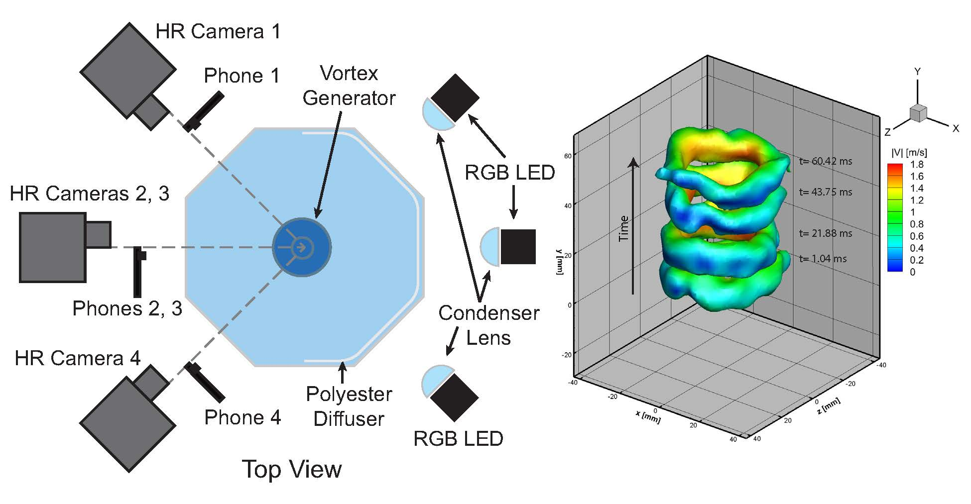
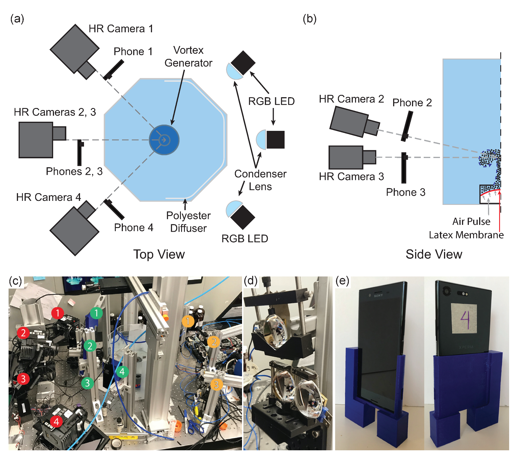
2.1. Overall Tomographic PIV Setup

Figure 1 shows the experimental setup, which is similar to our previous study [33]. The octagonal acrylic tank is filled with a mix of 60%–40% by volume of water-glycerol to better match the density of the seeding particles. This mixture has a density ρ = 1.12 g/cm³ and kinematic viscosity $\nu$ = 4.03 cSt. A 3D printed vortex generator is placed in the bottom of the tank. A latex membrane is stretched across the interior of the vortex generator and then a pulse of air synchronized with the cameras through a digital delay generator actuates the membrane emitting a vortex ring from the orifice. The liquid in the vortex ring generator is seeded beforehand with opaque black polyethylene particles with a diameter between 212–250 μm and material density ρ = 1.28 g/cm³. The particles are stirred inside the chamber allowing them to be dragged by the vortex ring.

The system is backlit by high-power LEDs (Luminus Devices Inc., Sunnyvale, CA, USA, PT-120) through diffusers to obtain a uniform background color intensity. Each LED is coupled with a 60 mm focal length aspheric condenser lens to focus the light onto the diffuser. The LEDs can be operated in either a continuous or pulsed mode using an LED driver board (Luminus Devices Inc., DK-136M-1). The pulse duration is controlled via a digital delay generator.

We use two camera systems simultaneously, a high-frame rate smartphone camera system operating at 960 fps at 720p HD resolution (Sony Xperia™ XZ), and a 4 K high-resolution camera system operating at 30 fps (RED Cinema Scarlet-X). Both systems contain four cameras each. Three of the cameras are positioned along a baseline with approximately 45° between cameras. This positions the optical axis of each camera perpendicular to a face of the octagonal tank reducing the effects of refraction. The fourth camera is positioned above the central camera and tilted downward at a small angle to overlap with the same field of view. The smartphones were mounted to the optics table using a custom, 3D printed holder.

The main difference from our previous study is the smartphone model and the system intended to synchronize and trigger the cameras. In the previous iteration, only three instants are captured with three different colors using a very long exposure (approximately 1 s) in all the cameras, thereby obtaining three time steps in a single image in each phone. In the current study we use the high-speed-video capability of the phones, which greatly increases the relevant applications for measurements in turbulent and non-steady flows. Therefore, we can use monochromatic illumination for time-resolved experiments, exposing one green flash of 80 μs in each frame, ensuring we capture the same instant in all sensors. We chose green color LED flashes due to the higher sensitivity for this wavelength in common CMOS color sensors that use a Bayer Filter, which have twice as many green pixels than red or blue. However, a color illumination scheme is required later in the study, where we perform a comparison with the concurrent higher spatial-resolution tomographic PIV system.

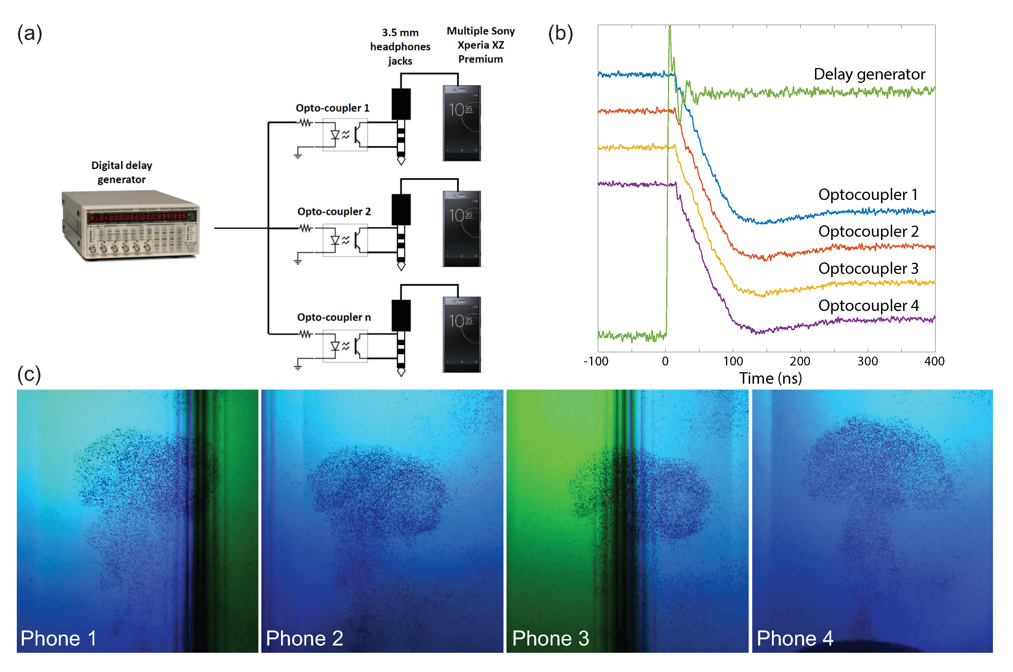
2.2. Smartphone Camera Triggering and Synchronization

Recent advances in smartphone technology have brought the capability of “slow-mo” videography to the general public. Here we use the Sony Xperia™ XZ Premium, released in June 2017, which includes a new sensor of 19 megapixels (Mpx) and the capability of recording “slow-mo” video at 960 fps at a lower pixel resolution $1280\times 720$ pixels equaling 0.92 Mpx. Some of the most relevant specifications are summarized in

Table 1. Summary of relevant specifications of the Sony Xperia™ XZ premium smartphone [34].

Platform	OS	Android 7.1 (Nougat)
	Chipset	Qualcomm MSM8998 Snapdragon 835
	CPU	Octa-core (4 × 2.45 GHz Kryo and 4 × 1.9 GHz Kryo)
	GPU	Adreno 540
Memory	Card Slot	microSD, up to 256 GB
	Internal	64 GB, 4 GB RAM
Cameras	Primary	19 Mpx, f/2.0, 25 mm, EIS (gyro), predictive phase detection and laser autofocus, LED flash
	Features	1/2.3-inch sensor size, 1.22 μm pixel size, geo-tagging, touch focus, face detection, HDR, panorama
	Video	2160p@30 fps, 720p@960 fps, HDR
	Secondary	13 Mpx, f/2.0, 22 mm, 1/3-inch sensor size, 1.12 μm pixel size, 1080 p

. The use of a new sensor technology named “Exmor RS™”, which has a memory stack on the camera sensor, allows faster image capturing and scanning space [34]. One of the drawbacks when recording high-speed video with these smartphones is that the phone is capable of recording only 177 successive frames. Further, synchronization of the recorded video in all the smartphones turns out to be a significant challenge.

In our prior work [33], we used a WiFi router to synchronize and trigger all of the smartphones followed by a long exposure time. Thus, the color flashes were able to “freeze” the same instant in all of the cameras. In contrast, recording at 960 fps results in a captured frame every 1.04 ms, which is faster than the typical response time achieved by the WiFi router used in the earlier study. To overcome this difficulty, we use the phone’s capability of triggering the camera with the pins present on the 3.5 mm audio jack by creating a short circuit between the GND and MIC pins. In our experiments, we use high-performance optocouplers (Fisher model 6N136-1443B) in parallel as relay switches between a TTL signal from a digital delay generator and an electrical input to the smartphones, which provides sufficiently fast temporal response as compared to a mechanical relay. Figure 2a shows a schematic of how the optocouplers are wired to the phones and connected to the delay generator. The time response characteristics are also essential for our high-speed application. Therefore, a test using the digital delay generator to check the response time of the optocoupler was carried out using a digital oscilloscope.

From Figure 2b, we see that the response time of the optocouplers is approximately 150 ns. This response is perfectly adequate for our relatively much lower frequency when recording video at 960 fps (exposure time of 1.04 ms). The fast response time will allow us in principle to synchronize the LED illumination and trigger the cameras simultaneously. However, when connecting the optocouplers to the smartphones and testing them with the LED system, we found that there is a random delay between the outgoing trigger pulse and the start of the frame captured by the each smartphone camera. This limits the number of frames that can be reconstructed since only frames that overlap in time for all the cameras can be used. Presumably, one could measure the delay between the trigger event and the start of recording for each smartphone and adjust the trigger time on the digital delay generator for each smartphone to obtain highly synchronized videos; however, in practice, we found no pattern or repeatability in the relative time offset between smartphones.

The previously mentioned problems may be caused by out-of-sync internal clocks in the different smartphones or the processing of background services typical for the Android OS. To eliminate the background process and applications running on each smartphone, we connected all four phones simultaneously to the same computer via a USB hub. Utilizing the Android Debug Bridge (ADB) [35], which is a command line application for sending shell commands to the Android OS, we were able to kill all of the background applications and processes using the force-stop command for each running process and application prior to triggering the “slow-mo” recording. Killing all of the processes coupled with the optocoupler triggering method increased the total number of frames overlapped by nearly three-fold. Routinely, we achieved between 160 and 170 out of 177 frames overlapping. If subsequent recordings were captured without killing all processes prior to each recording, the number of overlapped frames quickly decreased to less than half of the total number of frames. Unfortunately, even after killing all background processes, we still found no repeatable time offset between smartphones, which would have enabled an even higher degree of synchronization.

Using ADB shell commands also opens an additional cost-effective method to trigger the recordings. Once all of the camera applications are open and running, a volume down key event can be sent from the command-line simultaneously to all of the connected smartphones utilizing the xargs command. This method of triggering had slightly worse performance in achieving maximum frame overlap across all phones achieving routinely 125 to 150 overlapping frames; however, it performed about twice as well as the optocoupler triggering without killing the background applications and processes. The ADB also has an additional benefit of enabling a programmatic method of pulling the recorded videos from the smartphones to the computer terminal via a shell script.

To provide a synchronization reference point encoded in the video recordings, a blue LED is flashed once in the middle of the recording with an exposure time of 80 μs. This information will allow us to pair together and synchronize the recordings during post-processing.

An additional problem we found while testing is that the camera sensor scanning occasionally is out of phase with the illumination. These problems arise because of the rolling shutter nature of the smartphone sensor, in addition to the out-of-phase internal clocks between the smartphones. This produces dark stripes in the sensor or overlapped adjacent flashes in a single frame. To test this problem a green LED is flashed for a frame followed by blue and green LEDs simultaneously, finalizing only with green flashes. Some of the captured images of the vortex ring show overlapped instants in a single frame (see Figure 2c). For the current proof-of-concept study, we overcome this problem by trial and error until capturing in-phase images in all of the camera sensors. In order to completely eliminate this out-of-phase problem, one may need to modify the operating system or internal circuitry of all the smartphones to have a single internal clock controlling all of them simultaneously, which is beyond the scope of this work. Recent work by Ansari et al. [36] proposes a software solution for smartphones to capture still image sequences syncrhonized within 250 μs. However, significant development and extension would be needed to apply this technique to high-speed video capture.

The lack of control of the camera settings when using the high-speed video mode increases the difficulty of our experiment. Due to the commercial nature of these devices and the low exposure time, of each frame, as the consequence of the high frame rate, the camera application used by Sony gives very limited control to the end user. Parameters such as ISO, exposure time, manual focus, RAW capture, and so forth are not manually controlled and are set automatically to obtain optimum illumination of the “slow-mo” video. These features, in our case, produce out of focus images with a very high ISO (grainy images) or overexposed images. To overcome this problem, empirically we found that just before starting the recording we need to flash the LED’s for a few seconds in order to let the camera sensor adjust the parameters for the current lighting conditions.

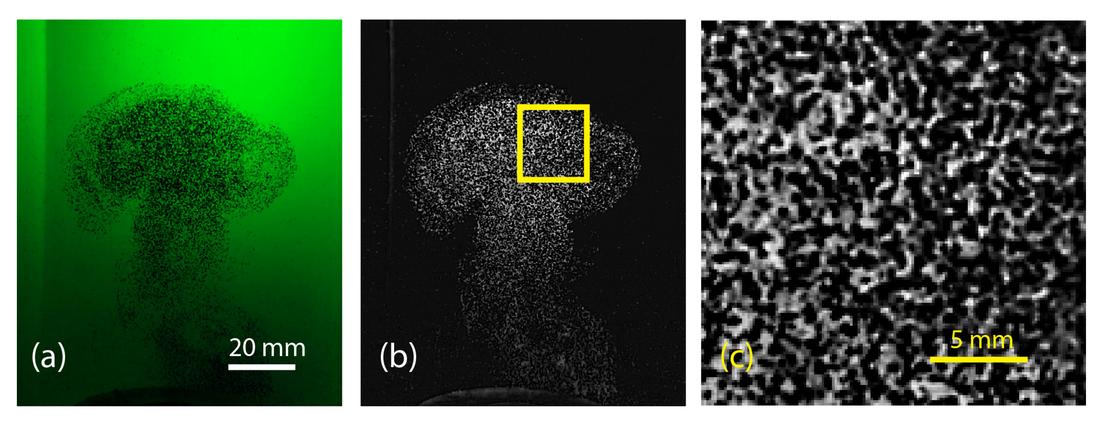
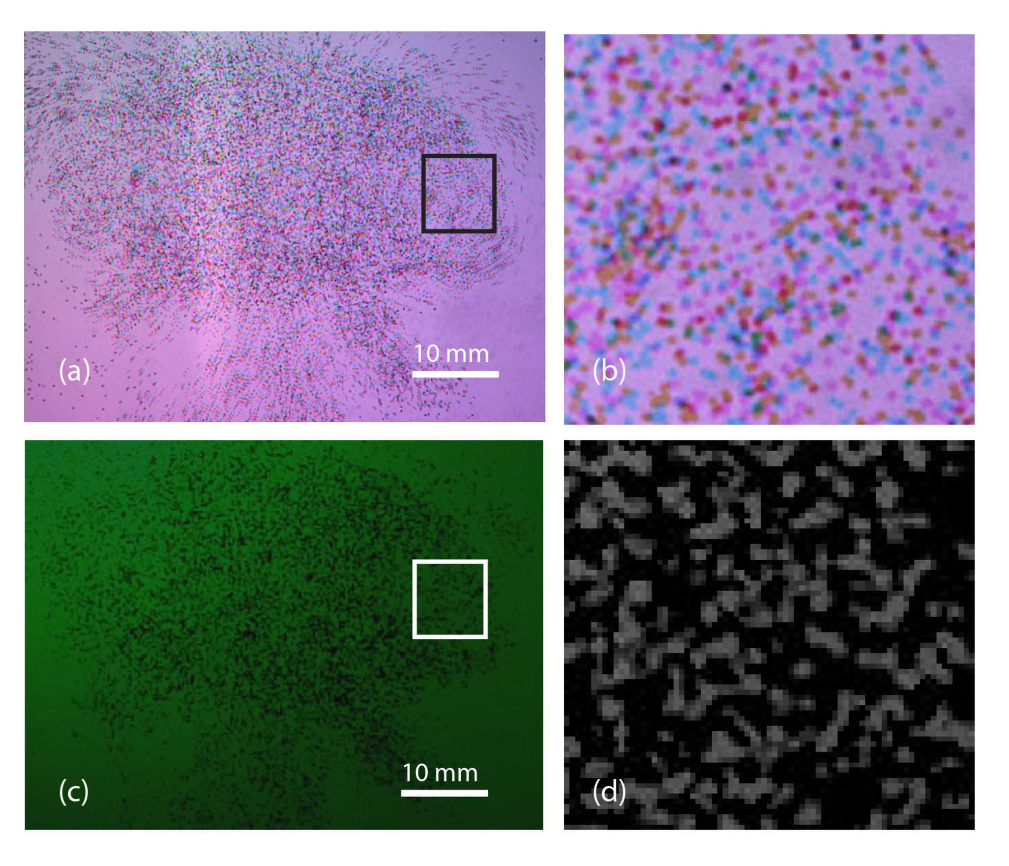
2.3. Image Pre-Processing

Figure 3 shows a typical image captured in the high-speed video mode. Here we can clearly see the vortex ring structure seeded with the black particles forming a “mushroom” shape (see Supplementary Video S1, here we can observe a recording at 960 fps of the vortex ring traveling upwards). The average density of particles inside the seeded region is $N\sim$ 0.08 particles per pixel (ppp). The source density or fraction of the image occupied by particles is $N_s\sim$ 0.5 for these experiments. Each particle is approximately 2 pixels in diameter. The maximum particle displacement between frames in the fastest regions is approximately 5 pixels near the vortex core. The non-uniform background (see Figure 3a) requires some image pre-processing to feed cleaner images to the DaVis software. We split the channels of the captured images, and only the green channel is processed. The open-source package, “Fiji”, is used to process the images and the “subtract background” command is used for this purpose. This command employs the “rolling ball” algorithm proposed by Sternberg [37]. A rolling ball radius of 20 pixels is used and smoothing is disabled to avoid blurring out individual particles. After removing the background, the images are inverted and enhanced by normalizing each frame by its maximum pixel value. Final images exhibit bright particles in a dark background as is required for the DaVis software (see Figure 3b,c). The captured images have a large pixel size of approximately 150 μm/px while our particles are approximately 200 μm in diameter.

The high particle density results in many particles that overlap. However, due to the robust nature of the Tomographic-PIV algorithm, this does not represent a major problem during the correlation process.

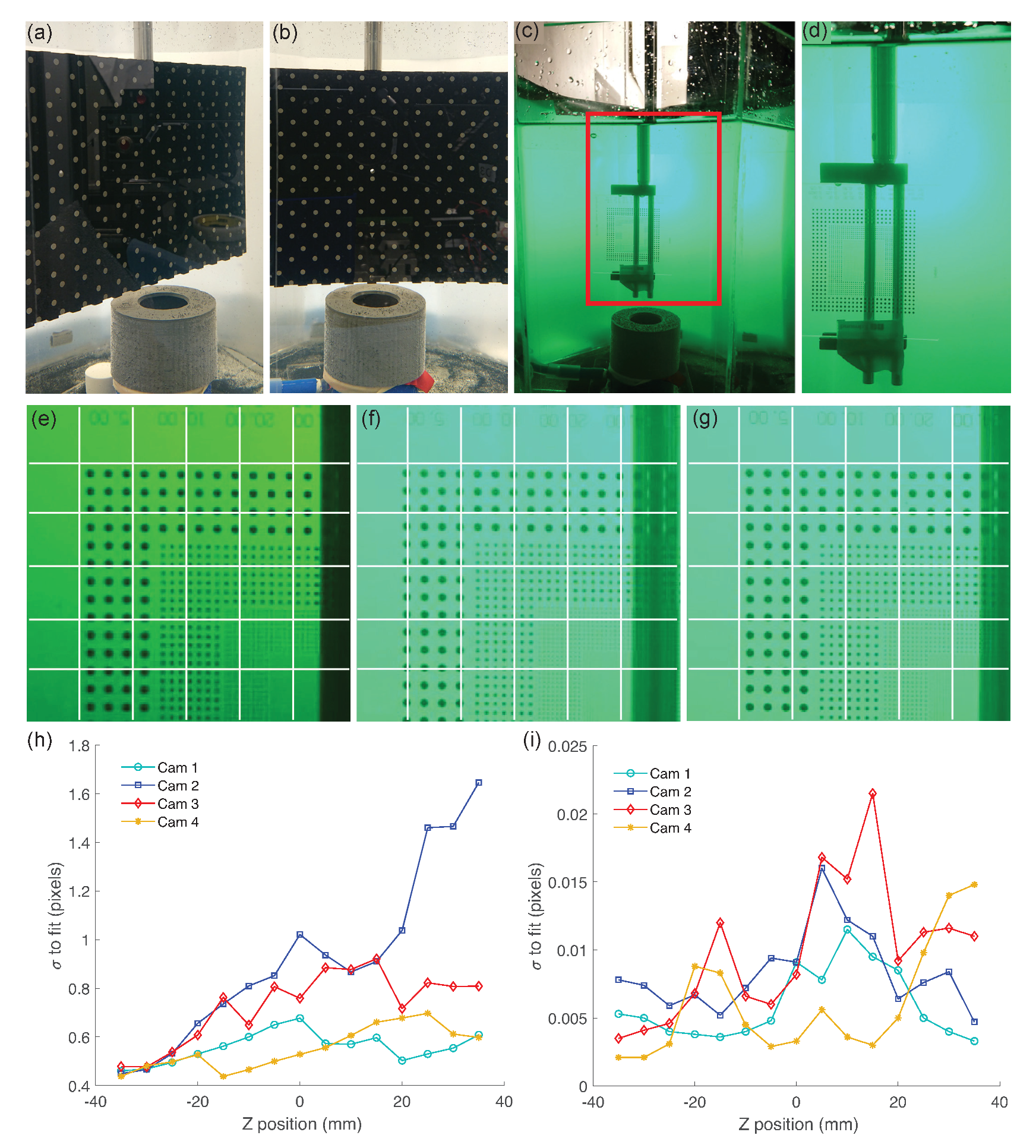
2.4. Tomographic PIV Calibration

A calibration plate Type 22 from LaVision, shown Figure 4a,b, is translated along the volume to be reconstructed, from $z=-35$ mm to $+35$ mm in 5 mm steps. However, since in high-speed mode the cameras focal plane is automatically adjusted, we capture full frame still calibration images of 19 Mpx in manual mode, Figure 4c. We fix the focal plane of each camera at the center of the vortex ring generator and carry out the calibration procedure.

To achieve the appropriate size calibration image, we first must downsample the 19 Mpx image and center crop it to match the dimensions and resolution of the high-speed video mode images, Figure 4d. Originally we assumed that a centered binning of $2\times 2$ in the central portion of the full frame image is used in high-speed video mode. In Figure 4f it is clearly observed that this $2\times 2$ binning produces an out of scale image compared with the high-speed mode image (Figure 4e). By testing the captured images with a dotted calibration target we found empirically that this is slightly off the center and the scaling of the image is not exactly 2, but 1.9267 as shown in Figure 4g. Therefore all the calibration images recorded at 19 Mpx resolution have to be adjusted and binned with a factor of 1.9267 × 1.9267 to reproduce the same field of view when recording in high-speed video mode.

The calibration is performed using the DaVis Tomographic PIV Software package. The initial calibration is carried out on all images of the calibration plate, and the initial calibration error estimation is obtained (see Figure 4h). A third order polynomial is used for the fit model. Camera 2 has the largest standard deviation from the calibration fit with a value of 1.65 pixels. However, the standard deviation is minimized by subsequently performing a self-calibration [38] in the DaVis software, where the reconstructed particles are triangulated and used directly to correct the calibrations via disparity maps. After three iterations of the self-calibration algorithm, the maximum standard deviation of the fit falls below 0.025 pixels as shown in Figure 4i.

2.5. Tomographic PIV Reconstruction and Correlation Procedures

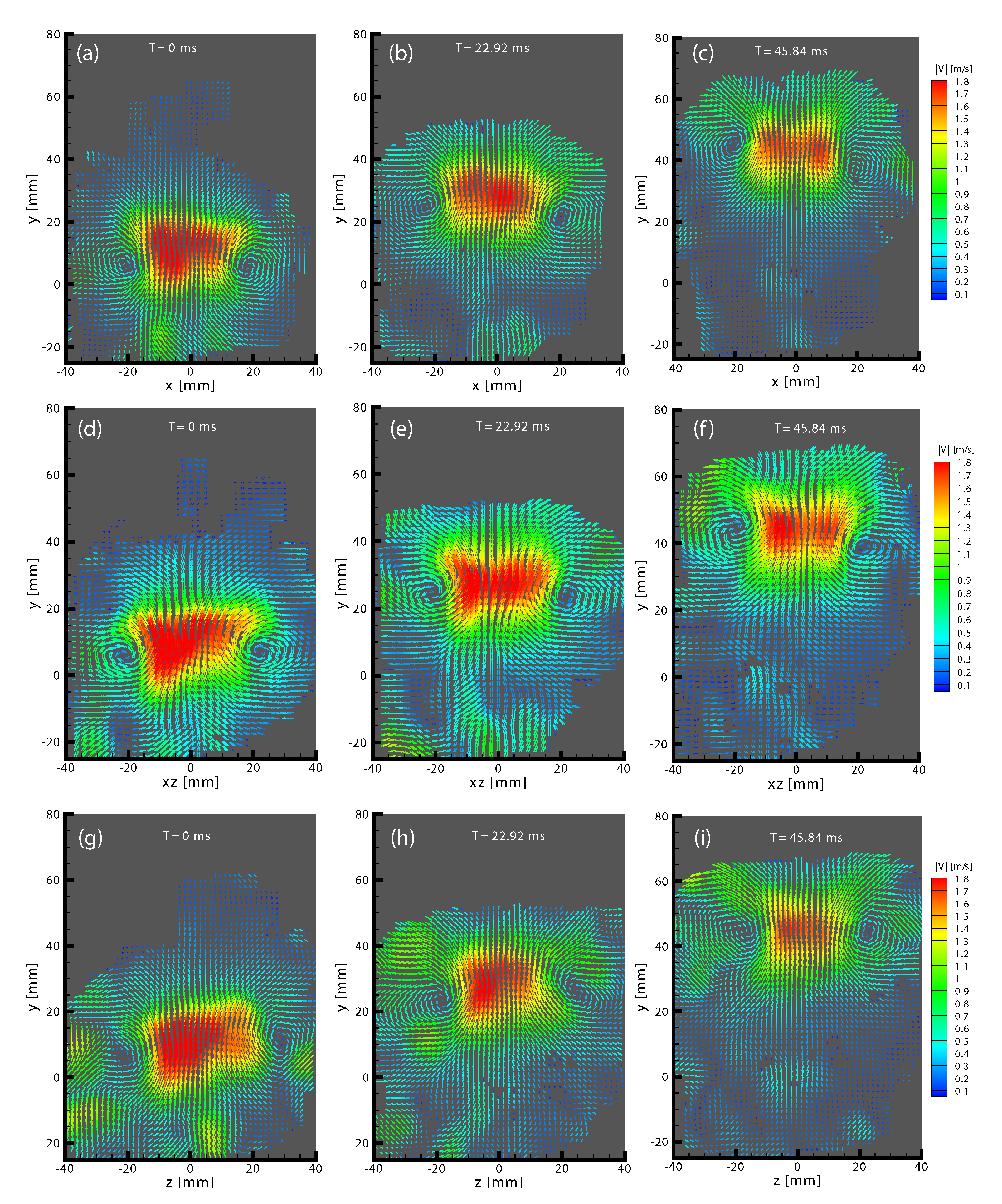
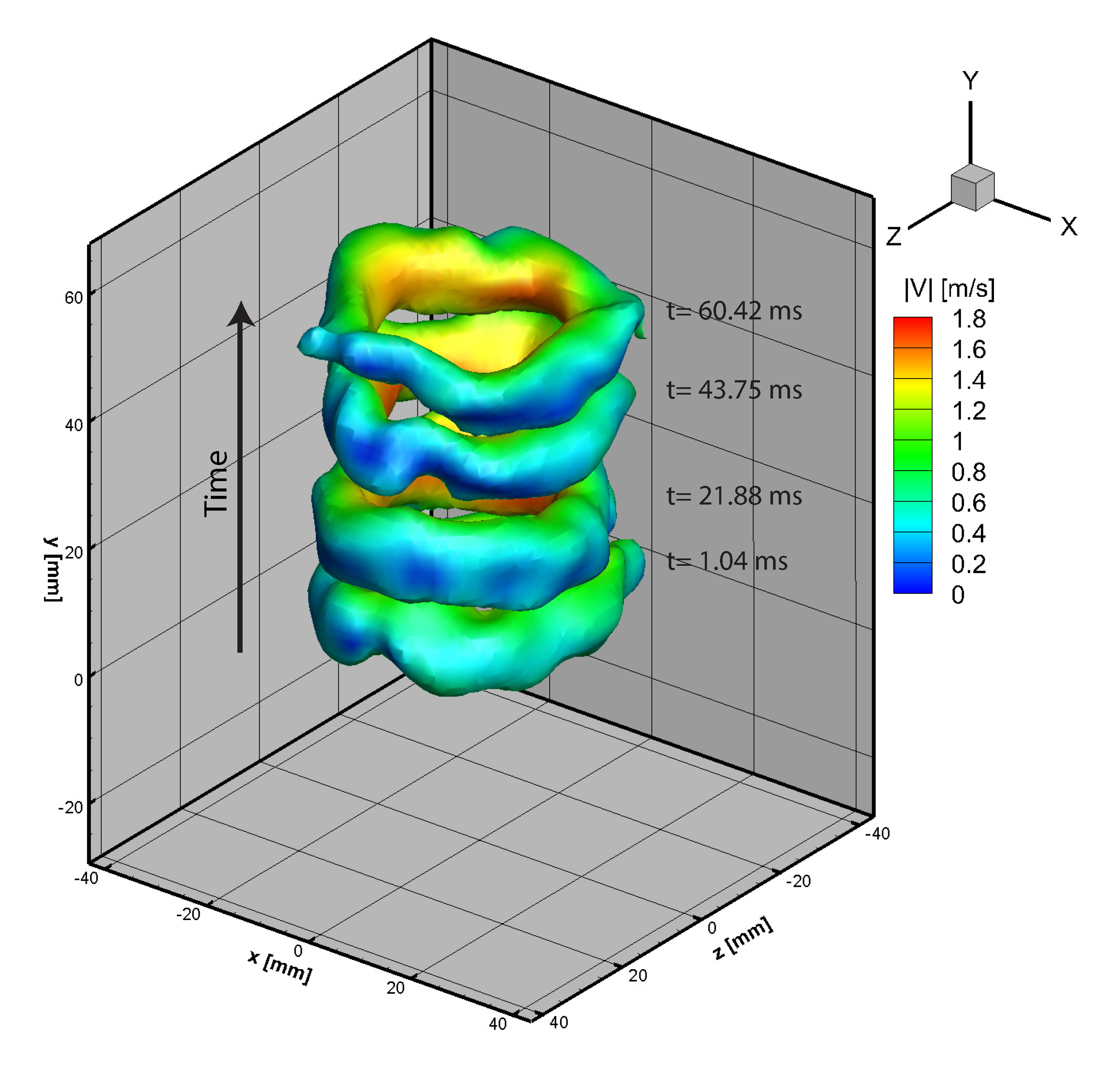
All the video frames are loaded into the DaVis Tomographic PIV Software, together with the calibration images. Particle locations are then reconstructed in a 3D volume using the Fast Multiplicative Algebraic Reconstruction Technique (MART) algorithm, which includes Multiplicative Line-Of-Sight (MLOS) initialization [39] and 10 iterations of the Camera Simultaneous (CS) MART algorithm first implemented by Gan et al. [40]. Therefore the volume of approximately 80 × 100 × 90 mm³ is discretized in the process to 500 × 625 × 593 voxels, having approximately 257 voxels/mm³. This is carried out for every time step.

Direct cross-correlation is carried out between subsequent reconstructions in order to estimate instantaneous velocity fields. This is done in four steps with an initial interrogation volume size of 128³ voxels with 8 × 8 × 8 volume binning. In order to refine the velocity fields, we reduce the interrogation volume size to 96³ voxels and binning of 4 × 4 × 4, 64³ voxels and 2 × 2 × 2 binning with a final interrogation volume size of 48³ voxels with no binning. All steps are repeated with two passes to reduce the number of outlier vectors with a 75% interrogation volume overlap and the final step has 3 passes. Gaussian smoothing of the velocity field is used between iterations to improve the quality of the vector field. As a result, we obtain a velocity field with approximately 1.6 mm vector pitch and approximately 91,500 vectors (in the seeded region).

3. Results

A sequence of 58 consecutive frames recorded at 960 fps, that is, Δt = 1.041 ms, was reconstructed to obtain 57 instantaneous, time-resolved velocity fields with a total of 5.2 × 10⁶ vectors. Figure 5 shows 2D cuts of the 3D velocity field at t = 0, 22.92, 45.84 ms for 3 different planes, the xy plane located at z = 0 mm, the vertical plane 45° from the x-axis, and the yz plane at x = 0 mm. As expected, the highest velocities occur in the center of the vortex ring. The core of the vortex ring is also clearly seen. To better visualize the core structure of the vortex ring, we calculate the vorticity from the velocity vectors. Figure 6 shows surfaces of isovorticity magnitude $\left|\omega \right|$ = 220 s⁻¹ through time, showing the vertical translation of the vortex ring structure. An animation of this process is also presented as Supplementary Video S2.

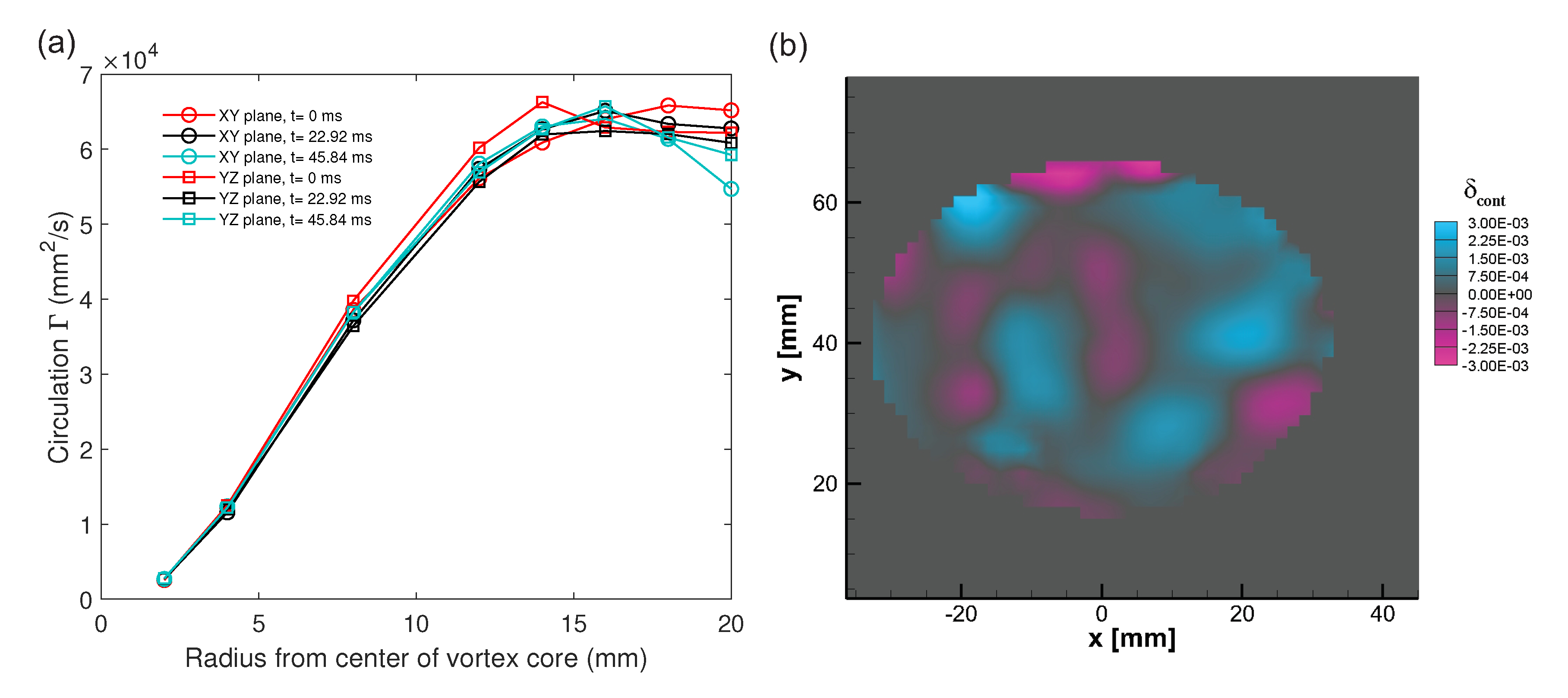
3.1. Circulation and Continuity Verification

To test the consistency of these results, we calculate the circulation and the residual from the continuity equation. We start with the circulation, $\mathsf{\Gamma }$, of the vortex ring, which should be constant around the periphery of the vortex ring.

This is calculated by computing the line integral of the tangential velocity around a closed circle, C, at several radii from the center of the vortex core ranging from 2 to 20 mm, that is,

$$\mathsf{\Gamma }={\oint }_C\mathbf{u}·dl.$$

(1)

Figure 7a shows calculated values of $\mathsf{\Gamma }$ on the $xy$ and $yz$ planes at three different times. As the radius from the vortex core increases, the circulation approaches a constant maximum of $\mathsf{\Gamma }=6.6\times {10}^4$ mm²/s irrespective of the plane. Below a radius of 16 mm, the circulation is nearly constant in space and time. Above 16 mm, the circulation is also nearly constant, but there is more variation in space and time. In all, the circulation is conserved supporting the consistency of the calculated velocity fields. We also estimate the Reynolds number of the vortex ring, $Re=\mathsf{\Gamma }/\nu$. Using the maximum circulation around the vortex core results in $Re=$ 16,500.

We next test the consistency of the velocity field results by verifying the conservation of mass for an incompressible fluid. Consistent results will yield a residual (${\delta }_{cont}$) of the continuity equation ($\nabla ·\mathbf{u}=0$) near zero. We normalize ${\delta }_{cont}$ by the inverse characteristic time scale of ($\tau =$ 0.022 s) which is the ratio of the vortex ring diameter ($D=$ 0.04 m) divided by the maximum velocity magnitude ($\left|V\right|=$ 1.8 m/s), that is, ${\delta }_{cont}=\nabla ·\mathbf{u}(D/|V\left|\right)$. Figure 7b shows the residual in the $xy$ central plane at $t=43.75$ ms. The largest magnitude of the normalized residual shown in the plot is ${\delta }_{cont}=3\times {10}^{-3}$, the mean value is $-2.79\times {10}^{-5}$ and the RMS value is $1.29\times {10}^{-3}$. Considering all velocity fields across every timestep the mean normalized residual is $7.08\times {10}^{-5}$ with an RMS value of $7.39\times {10}^{-4}$. This low value of the mean residual gives us further confidence in the veracity of the velocity fields.

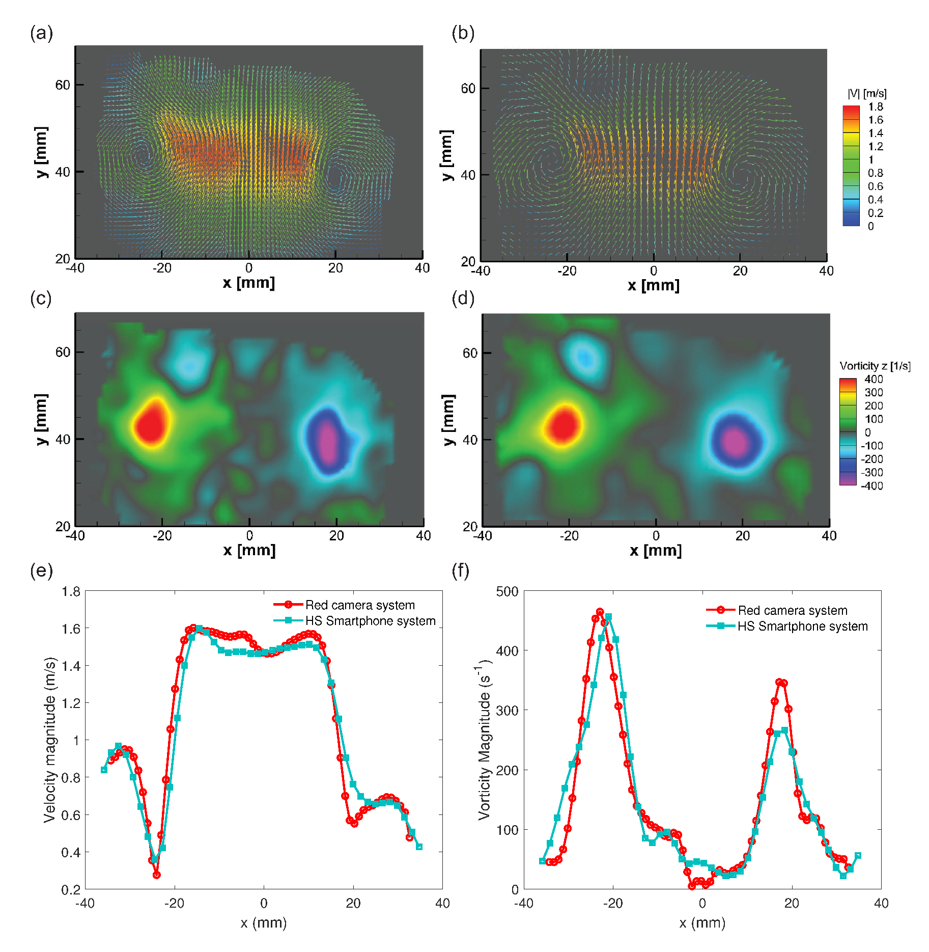
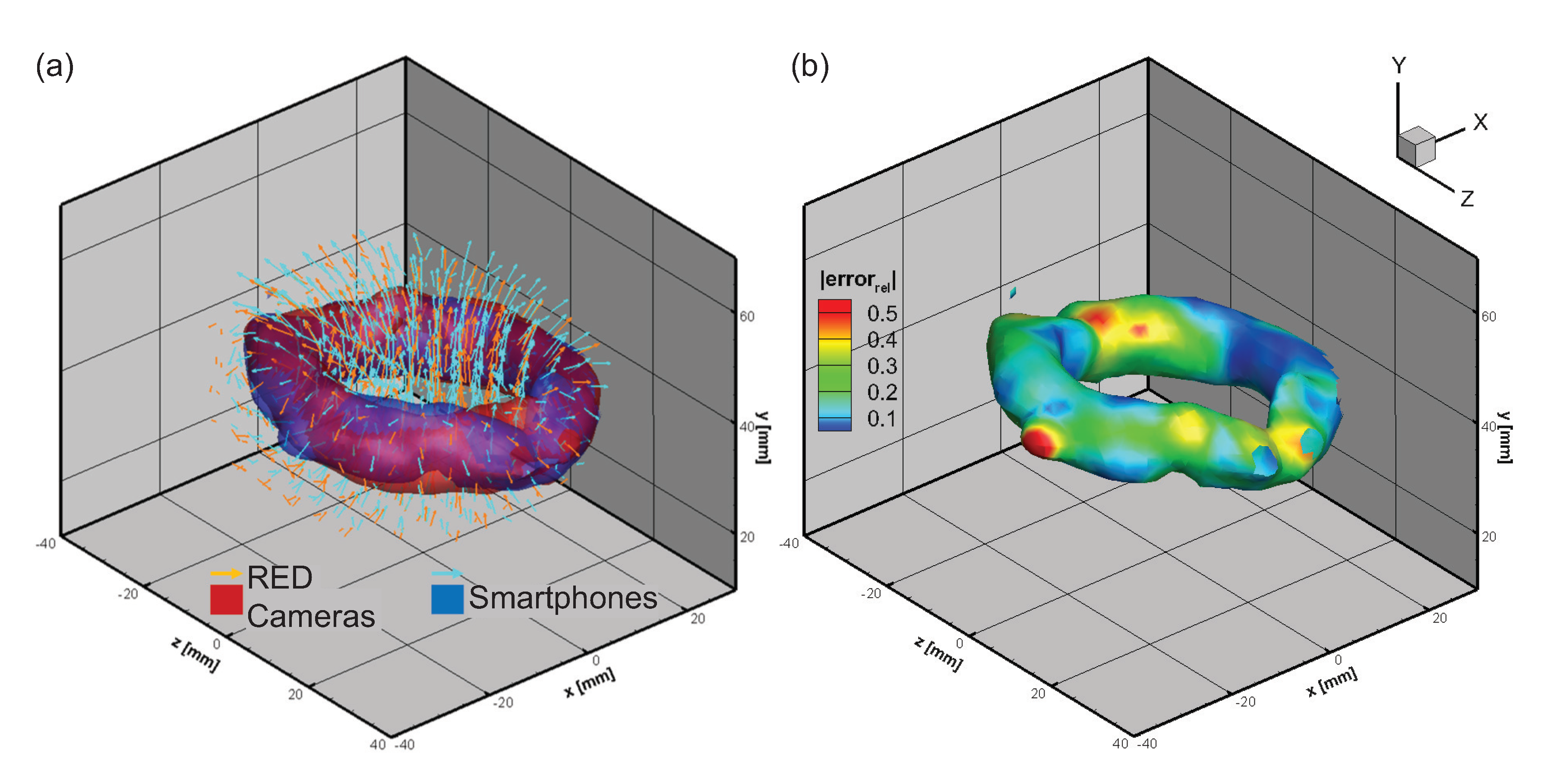
3.2. Comparison with High Resolution Tomographic PIV System

To further ascertain the accuracy of these measurements, we make a benchmark comparison between our high-speed smartphone system and a simultaneous ultra-high resolution camera system measurements. The high-resolution cameras used for this benchmark are 4 RED Cinema Scarlet-X cameras synchronized with a Lockit ACL 204 timecode and sync generator. These cameras record video with 4 K resolution (3840 pixels × 2160 pixels); however, at this resolution the frame-rate is restricted to only 30 fps. To overcome the mismatch in frame rate between the two systems, we encode the time in the color of three LED flashes as done in our previous work [33]; this will allow us to record the position of all the particles at the same instant in both systems (smartphones and RED Cameras) concurrently. The RED cinema cameras are placed close to the location of each of the smartphones (Figure 1). The same calibration plate, type 22, is used to obtain calibration images in both the smartphones and RED Cinema cameras yielding the same coordinate system in both systems. The results of this concurrent experiment are a single image containing the three time steps for each RED Cinema camera (3840 × 2160 pixels), while the smartphone system will produce three consecutive frames in time (1280 × 720 pixels) for each camera. This is approximately nine times difference in total image resolution or number of pixels, allowing us to reconstruct a very detailed velocity field as a reference using the Red Cinema cameras.

We flash a green, then a blue and finally a red LED subsequently with a Δt = 1/960 s and an 80 μs exposure time. This allows us to compare two different velocity fields produced by each system independently. For the RED cameras, the captured raw images have to be processed to separate the color channels, that is, the different time steps, following the method of Aguirre-Pablo et al. [33]. In short, raw images are used which are acquired using the GRBG Bayer filter array on the camera sensor before the interpolation to create the three separate color channels is performed. The images are then separated into colors based on the pixel location on the sensor and the corresponding color in the Bayer filter filling in gaps with a zero intensity. Next each color channel is interpolated using the demosaic method proposed by Malvar et al. [41]. Additionally, a “Zero-time delay” correction is applied to reduce the systematic errors that arise from chromatic aberrations [33,42]. The images captured by the smartphones follow the same post-processing flow as specified in the methods section. Figure 8 shows a comparison of raw images of a vortex ring captured on both the systems demonstrating the difference in resolution.

For the RED Cinema camera system, the 3D reconstruction procedure yields 2025 × 2025 × 1922 voxels for each time step. The same process for the smartphone camera system yields 586 × 586 × 557 voxels. The volume reconstructed in both cases is approximately 80 × 80 × 76 mm³. The direct cross-correlation procedure to obtain velocity vectors for both systems is the same as described previously; however, the interrogation volume size differs between the RED Cinema cameras and the smartphone systems. For the RED Cinema cameras, the final correlation volume size is ${104}^3$ voxels with 75% overlap, whereas for the Xperia™ system the final interrogation volume size is ${48}^3$ voxels with 75% overlap. This produces approximately 4 times more 3D vectors for the RED camera system.

We compare qualitatively the planar velocity fields in Figure 9a,b and the out-of-plane azimuthal vorticity in Figure 9c,d in the central $xy$ plane. The main qualitative features such as the location of the vortex core, velocity, and vorticity magnitude are comparable for both systems. However, the relatively lower resolution in the case of the smartphones is evident from this figure. Further comparison is carried out at a horizontal line (at y = 44 mm) that cuts one side of the vortex core (since the vortex core is not completely horizontal). Despite the high-velocity gradients in the area, Figure 9e shows close similarity between the velocity profiles reconstructed by the two independent systems. Figure 9f shows similar results for the isovorticity magnitude values along the same line. We highlight that the largest errors are due to slight offsets in the vortex core location combined with the strong velocity gradients close to the outer edge of the cores.

In Figure 10a, we present an overlay of an isovorticity surface, $\left|\omega \right|$ = 210 s⁻¹, and velocity vectors obtained with both systems at the same instant. Visually, the isovorticity surfaces and velocity vectors are comparable and describe the same qualitative features of the vortex ring. Nevertheless, one has to keep in mind that the spatial resolution of the velocity field produced by the smartphones is approximately 1/4 of the spatial resolution of the RED cameras. We further perform a node-by-node comparison and obtain an error estimation of the velocity components. Since the resolution of the two systems is different, the RED camera results are downscaled by linear interpolation to match the same grid size as the smartphone system case (i.e., from the original 1.03 × 1.03 × 1.03 mm³ mesh to a 1.64 × 1.64 × 1.64 mm³ per node). This interpolation allows us to obtain the relative error vector of the velocity at every node. The error vector is normalized by the maximum magnitude of velocity (herein, 1.8 m/s). Figure 10b presents an isovorticity surface of 210 s⁻¹ colored by the relative error, this way we can detect the regions where the error is higher. One has to keep in mind that regions close to the vortex core have the greatest velocity gradient. The values presented in the plot represent an upper bound of our error.

4. Discussion and Conclusions

In this study we have demonstrated the use of smartphones, capable of recording high-speed video at 960 fps, for time-resolved measurements in a Tomographic PSV setup. The proof of concept presented herein will facilitate the study of turbulent flows without the need for expensive specialized equipment. The camera and LED illumination system are similar to the one proposed in our previous study [33]. However, synchronization of the cameras is critical for this section due to the high-speed nature of the technique and limited number of frames recorded at 960 fps. Synchronization was accomplished by using high-performance optocouplers that have a typical response time of 150 ns to a TTL pulse from a signal generator. This method resulted in the overlap of ≈90–95% of the frames in all cameras; however, many challenges still exist, such as out of phase clocks of the sensors, random delay in the camera recording startup and manual control of the camera parameters (e.g., exposure and focus). Nevertheless, it is natural to think that future Android and iOS Camera API releases may include manual control functionality while in high-speed mode, as more smartphones integrate a high frame-rate sensor. Extension of software synchronization methods such as Ansari et al. [36] could overcome the synchronization challenges.

To test the proposed technique, measurements of a vortex ring with approximately 40 mm in diameter were carried out. The Reynolds number of the tested rings is $Re=\mathsf{\Gamma }/\nu =$ 16,000. The maximum velocity magnitude measured in these rings is approximately 1.8 m/s. A total of approximately 5.2 million individual vectors are reconstructed over the whole time sequence (approximately 90,000 vectors per time step) with a pitch of 1.6 mm in every direction. The results obtained are then verified with concurrent secondary measurements, in a similar way to Aguirre-Pablo et al. [33]. However, in this work we expand the comparison to the whole 3D flow field. The increase of circulation as a function of the radial distance from the core is compared at different time steps and vertical planes, that is, circulation around the core in different vertical planes, as well as the verification of the closure of the continuity equation yielding similar profiles in all cases. Continuity verification produced a mean normalized residual of ${\delta }_{cont}=6.27\times {10}^{-4}$.

Furthermore, concurrent experiments measuring the vortex ring with the Tomo-PIV smartphone system and an ultra-high resolution (4 K resolution) system using four RED cinema cameras are carried out. The RED cinema system allowed us to benchmark our result to a simultaneous much higher spatial resolution velocity field. However, RED Cinema cameras can record only up to 30 fps at the 4 K resolution, for this reason, we use the technique proposed by Aguirre-Pablo et al. [33] using colored shadows to encode time in both cases. The comparison shows very similar qualitative and quantitative results. As shown in Figure 9 and Figure 10, one can notice the similarity of the results produced for both systems (4 K system and smartphone system). We compare the velocity field, velocity magnitude, vorticity field magnitude and their 3D spatial distribution.

Our proof-of-concept demonstration reduces the cost of the hardware required for full 3D-3C, time resolved Tomographic PSV measurements for turbulent flows by piggy-backing on the economics of scale for consumer electronics. The hardware total cost is approximately $6000 USD, including LED illumination and its drivers, opto-coupler unit, and four smartphones capable of high speed video. The cost is reduced by approximately 30 times when compared to the specialized equipment typically used in Tomographic PIV. Additionally, the portability of the system proposed herein, enables flow measurements in limited space areas.

The system proposed in this work, will lower the entry bar for 3D flow measurements in education, scientific research and industrial applications. However, the most needed improvement in the hardware is a variable-zoom lens. In the “slow-mo” recording mode, manual control of the focus and option to store the video clip in RAW format, will improve color-splitting of the frames and allow multiple light-pulses per frame, thereby increasing the effective frame-rate, using our earlier methods from Aguirre-Pablo et al. [33].

References

1. Adrian, R.J. Particle-imaging techniques for experimental fluid mechanics. Ann. Rev. Fluid Mech. 1991, 23, 261–304. [Google Scholar] [CrossRef]
2. Westerweel, J.; Elsinga, G.E.; Adrian, R.J. Particle image velocimetry for complex and turbulent flows. Ann. Rev. Fluid Mech. 2013, 45, 409–436. [Google Scholar] [CrossRef]
3. Willert, C.E.; Gharib, M. Digital particle image velocimetry. Exp. Fluids 1991, 10, 181–193. [Google Scholar] [CrossRef]
4. Hori, T.; Sakakibara, J. High-speed scanning stereoscopic PIV for 3D vorticity measurement in liquids. Meas. Sci. Technol. 2004, 15, 1067. [Google Scholar] [CrossRef]
5. Elsinga, G.E.; Scarano, F.; Wieneke, B.; van Oudheusden, B.W. Tomographic particle image velocimetry. Exp. Fluids 2006, 41, 933–947. [Google Scholar] [CrossRef]
6. Scarano, F. Tomographic PIV: Principles and practices. Meas. Sci. Technol. 2012, 24, 012001. [Google Scholar] [CrossRef]
7. Belden, J.; Truscott, T.T.; Axiak, M.C.; Techet, A.H. Three-dimensional synthetic aperture particle image velocimetry. Meas. Sci. Technol. 2010, 21, 125403. [Google Scholar] [CrossRef] [Green Version]
8. Bomphrey, R.J.; Henningsson, P.; Michaelis, D.; Hollis, D. Tomographic particle image velocimetry of desert locust wakes: Instantaneous volumes combine to reveal hidden vortex elements and rapid wake deformation. J. R. Soc. Interface 2012, 9, 3378–3386. [Google Scholar] [CrossRef] [Green Version]
9. Langley, K.R.; Hardester, E.; Thomson, S.L.; Truscott, T.T. Three-dimensional flow measurements on flapping wings using synthetic aperture PIV. Exp. Fluids 2014, 55, 1831. [Google Scholar] [CrossRef]
10. Casey, T.A.; Sakakibara, J.; Thoroddsen, S.T. Scanning tomographic particle image velocimetry applied to a turbulent jet. Phys. Fluids 2013, 25, 025102. [Google Scholar] [CrossRef] [Green Version]
11. Ianiro, A.; Lynch, K.P.; Violato, D.; Cardone, G.; Scarano, F. Three-dimensional organization and dynamics of vortices in multichannel swirling jets. J. Fluid Mech. 2018, 843, 180. [Google Scholar] [CrossRef]
12. Mugundhan, V.; Pugazenthi, R.; Speirs, N.B.; Samtaney, R.; Thoroddsen, S.T. The alignment of vortical structures in turbulent flow through a contraction. J. Fluid Mech. 2020, 884, A5. [Google Scholar] [CrossRef] [Green Version]
13. Saaid, H.; Voorneveld, J.; Schinkel, C.; Westenberg, J.; Gijsen, F.; Segers, P.; Verdonck, P.; de Jong, N.; Bosch, J.G.; Kenjeres, S.; et al. Tomographic PIV in a model of the left ventricle: 3D flow past biological and mechanical heart valves. J. Biomech. 2019, 90, 40–49. [Google Scholar] [CrossRef] [PubMed]
14. Willert, C.; Gharib, M. Three-dimensional particle imaging with a single camera. Exp. Fluids 1992, 12, 353–358. [Google Scholar] [CrossRef]
15. Tien, W.H.; Dabiri, D.; Hove, J.R. Color-coded three-dimensional micro particle tracking velocimetry and application to micro backward-facing step flows. Exp. Fluids 2014, 55, 1684. [Google Scholar] [CrossRef]
16. Kreizer, M.; Liberzon, A. Three-dimensional particle tracking method using FPGA-based real-time image processing and four-view image splitter. Exp. Fluids 2011, 50, 613–620. [Google Scholar] [CrossRef]
17. Gao, Q.; Wang, H.P.; Wang, J.J. A single camera volumetric particle image velocimetry and its application. Sci. China Technol. Sci. 2012, 55, 2501–2510. [Google Scholar] [CrossRef]
18. Cenedese, A.; Cenedese, C.; Furia, F.; Marchetti, M.; Moroni, M.; Shindler, L. 3D particle reconstruction using light field imaging. In Proceedings of the International Symposium on Applications of Laser Techniques to Fluid Mechanics, Lisbon, Portugal, 9–12 July 2012. [Google Scholar]
19. Skupsch, C.; Brücker, C. Multiple-plane particle image velocimetry using a light-field camera. Opt. Express 2013, 21, 1726–1740. [Google Scholar] [CrossRef] [Green Version]
20. Shi, S.; Ding, J.; Atkinson, C.; Soria, J.; New, T.H. A detailed comparison of single-camera light-field PIV and tomographic PIV. Exp. Fluids 2018, 59, 46. [Google Scholar] [CrossRef]
21. Rice, B.E.; McKenzie, J.A.; Peltier, S.J.; Combs, C.S.; Thurow, B.S.; Clifford, C.J.; Johnson, K. Comparison of 4-camera Tomographic PIV and Single-camera Plenoptic PIV. In Proceedings of the 2018 AIAA Aerospace Sciences Meeting, Kissimmee, FL, USA, 8–12 January 2018; p. 2036. [Google Scholar]
22. Ido, T.; Shimizu, H.; Nakajima, Y.; Ishikawa, M.; Murai, Y.; Yamamoto, F. Single-camera 3-D particle tracking velocimetry using liquid crystal image projector. In Proceedings of the ASME/JSME 2003 4th Joint Fluids Summer Engineering Conference, Honolulu, HI, USA, 6–10 July 2003; pp. 2257–2263. [Google Scholar]
23. Zibret, D.; Bailly, Y.; Prenel, J.P.; Malfara, R.; Cudel, C. 3D flow investigations by rainbow volumic velocimetry (RVV): Recent progress. J. Flow Vis. Image Process. 2004, 11. [Google Scholar] [CrossRef]
24. McGregor, T.J.; Spence, D.J.; Coutts, D.W. Laser-based volumetric colour-coded three-dimensional particle velocimetry. Opt. Lasers Eng. 2007, 45, 882–889. [Google Scholar] [CrossRef]
25. Ruck, B. Colour-coded tomography in fluid mechanics. Opt. Laser Technol. 2011, 43, 375–380. [Google Scholar] [CrossRef]
26. Xiong, J.; Idoughi, R.; Aguirre-Pablo, A.A.; Aljedaani, A.B.; Dun, X.; Fu, Q.; Thoroddsen, S.T.; Heidrich, W. Rainbow particle imaging velocimetry for dense 3D fluid velocity imaging. ACM Trans. Graphics (TOG) 2017, 36, 36. [Google Scholar] [CrossRef] [Green Version]
27. Xiong, J.; Aguirre-Pablo, A.A.; Idoughi, R.; Thoroddsen, S.T.; Heidrich, W. Rainbow PIV with improved depth resolution—Design and comparative study with TomoPIV. Meas. Sci. Technol. 2020. [Google Scholar] [CrossRef]
28. Aguirre-Pablo, A.; Aljedaani, A.B.; Xiong, J.; Idoughi, R.; Heidrich, W.; Thoroddsen, S.T. Single-camera 3D PTV using particle intensities and structured light. Exp. Fluids 2019, 60, 25. [Google Scholar] [CrossRef] [Green Version]
29. Willert, C.; Stasicki, B.; Klinner, J.; Moessner, S. Pulsed operation of high-power light emitting diodes for imaging flow velocimetry. Meas. Sci. Technol. 2010, 21, 075402. [Google Scholar] [CrossRef] [Green Version]
30. Buchmann, N.A.; Willert, C.E.; Soria, J. Pulsed, high-power LED illumination for tomographic particle image velocimetry. Exp. Fluids 2012, 53, 1545–1560. [Google Scholar] [CrossRef]
31. Estevadeordal, J.; Goss, L. PIV with LED: Particle shadow velocimetry (PSV) technique. In Proceedings of the 43rd AIAA Aerospace Sciences Meeting and Exhibit, Reno, NV, USA, 10–13 January 2005; p. 37. [Google Scholar]
32. Cierpka, C.; Hain, R.; Buchmann, N.A. Flow visualization by mobile phone cameras. Exp. Fluids 2016, 57, 108. [Google Scholar] [CrossRef]
33. Aguirre-Pablo, A.A.; Alarfaj, M.K.; Li, E.Q.; Hernández-Sánchez, J.F.; Thoroddsen, S.T. Tomographic Particle Image Velocimetry using Smartphones and Colored Shadows. Sci. Rep. 2017, 7, 3714. [Google Scholar] [CrossRef] [Green Version]
34. Sonymobile. Sony Xperia XZ Premium. 2017. Available online: https://www.sonymobile.com/global-en/products/phones/xperia-xz-premium/ (accessed on 1 May 2017).
35. Android Debug Bridge (adb): Android Developers. Available online: https://developer.android.com/studio/command-line/adb (accessed on 20 March 2020).
36. Ansari, S.; Wadhwa, N.; Garg, R.; Chen, J. Wireless software synchronization of multiple distributed cameras. In Proceedings of the 2019 IEEE International Conference on Computational Photography (ICCP), Tokyo, Japan, 15–17 May 2019; pp. 1–9. [Google Scholar]
37. Sternberg, S.R. Biomedical image processing. Computer 1983, 16, 22–34. [Google Scholar] [CrossRef]
38. Wieneke, B. Volume self-calibration for 3D particle image velocimetry. Exp. Fluids 2008, 45, 549–556. [Google Scholar] [CrossRef]
39. Atkinson, C.; Soria, J. An efficient simultaneous reconstruction technique for tomographic particle image velocimetry. Exp. Fluids 2009, 47, 553. [Google Scholar] [CrossRef]
40. Gan, L.; Cardesa-Duenas, J.I.; Michaelis, D.; Dawson, J. Comparison of tomographic PIV algorithms on resolving coherent structures in locally isotropic turbulence. In Proceedings of the 16th International Symposium on Applications of Laser Techniques to Fluid Mechanics, Lisbon, Portugal, 9–12 July 2012. [Google Scholar]
41. Malvar, H.S.; He, L.-W.; Cutler, R. High-quality linear interpolation for demosaicing of Bayer-patterned color images. In Proceedings of the 2004 IEEE International Conference on Acoustics, Speech, and Signal Processing, Montreal, QC, Canada, 17–21 May 2004; Volume 3, pp. iii-485–iii-488. [Google Scholar]
42. McPhail, M.J.; Fontaine, A.A.; Krane, M.H.; Goss, L.; Crafton, J. Correcting for color crosstalk and chromatic aberration in multicolor particle shadow velocimetry. Meas. Sci. Technol. 2015, 26, 025302. [Google Scholar] [CrossRef] [PubMed]
Figure 1. (a) Top view sketch of the experimental setup showing the positioning of smartphones, high-resolution (HR) cameras, and LED back-lighting around an octagonal tank. (b) Side-view sketch showing the vertical positioning of the central cameras and a cross-section of the vortex generator at the tank centerline. (c) Photograph of experimental setup. HR Red Cinema cameras are labeled with red circles, while the Xperia smartphones are labeled with green circles and the LED clusters are labeled with orange circles. (d) Close-up detailed photograph of an RGB LED cluster with lenses. (e) Detail photographs of the custom, in-house 3D printed smartphone holder to stiffly mount the smartphones via aluminum struts to the optical table.
Applsci 10 07094 g001
Figure 2. (a) Schematic representation of the synchronization system, proposed for simultaneous capturing high-speed video at 960 fps by multiple smartphone cameras. The TTL signal is generated by a digital delay generator. This signal is sent in parallel to multiple optocouplers that trigger the Xperia™ XZ cameras through the headphone jack. (b) Signal characterization of the optocouplers versus the trigger signal from the digital delay generator. The typical response time of the optocoupler is approximately 150 ns. (c) Images of a vortex ring captured close to the same time. One can note that the scanning of the sensor produces overlapped flashes in phones 1 and 3. Whereas for phones 2 and 4 the flash is in phase with the recorded frame.
Applsci 10 07094 g002
Figure 3. (a) Single frame of a Vortex ring from a High-speed video. (b) Post-processed image. (c) Magnification of a sampled area inside the yellow region in (b).
Applsci 10 07094 g003
Figure 4. (a,b) Smartphone images captured in the manual mode for the calibration plate at z = 0 mm by (a) left camera, phone 1, and (b) central bottom camera, phone 3. The gray cylinder at the bottom is the vortex ring generator. (c,d) Top central camera, phone 2, view of a dotted calibration target located at the central plane of the vortex ring. (c) Captured with manual settings at 19 Mpx resolution. (d) Image of 2 × 2 binned image from 19 Mpx resolution and centered cropped to 1280 × 720 pixels (see the red region in (c)). (eg) Region of Interest (ROI) zoom ( 253 × 247 pixels) from the dotted calibration target. (e) High-speed video recording mode, (f) centered binning of 2 × 2 with top left corner located at x = 624 and y = 588 px (centered down-scaled image) (g) Binning of 1.9267 × 1.9267 with top left corner located in x = 648 and y = 590 px of the binned image. A rectangular grid is shown for comparison. (h) Initial standard deviation of the calibration fit. (i) Final calibration standard deviation after three iterations of the self-calibration algorithm.
Applsci 10 07094 g004
Figure 5. (ac) Two dimensional x y cuts through the center of the vortex ring, showing the instantaneous velocity field. (df) Two dimensional vertical cut of the instantaneous velocity field in a 45-degree x z plane. (gi) Two-dimensional y z cut of the instantaneous velocity field at the center of the vortex ring (note that this plane is not directly visible and is perpendicular to the central camera sensors). Different times are plotted from left to right (0, 22.92 and 45.84 ms respectively, showing the upward translation of the vortex ring). Vectors are colored by their velocity magnitude.
Applsci 10 07094 g005
Figure 6. Time evolution of surfaces with isovorticity magnitude of | ω | = 220 s−1. The color of the surface represents the velocity magnitude where we can see that the inner surface near the axis of symmetry of the vortex ring, has a larger velocity.
Applsci 10 07094 g006
Figure 7. (a) Circulation, Γ , versus radius from the vortex core; data is presented for 2D cuts of planes x y and y z (the latter one is not visible to the central cameras) colored by the three different instants t = 0 (red), 22.92 (black) and 45.84 (blue) ms. The Reynolds number for this vortex ring is R e 16,500. (b) Contour plot of the normalized residual δ c o n t obtained from the continuity equation · u = 0 at the XY central plane ( z = 0 ) of the vortex ring at t = 43.75 ms.
Applsci 10 07094 g007
Figure 8. Raw images from the central camera (camera 3) of a vortex ring captured simultaneously by (a) a RED 4k video camera and (c) an Xperia™ smartphone. Panels (b,d) show the corresponding magnified regions marked in the respective squares in panels (a,c). One can note the difference in the resolution of the two systems. The viewing angles for (a,c) are slightly different. Therefore, the images are not fully comparable.
Applsci 10 07094 g008
Figure 9. (a,b) Side by side comparison of velocity vectors colored by velocity magnitude on the center x y plane for (a) high-resolution RED camera system and (b) high-speed smartphone camera system. (c,d) Contour plots of vorticity magnitude are presented for (c) the high-resolution camera system and (d) the high-speed smartphone camera system. Visually one can notice the difference in spatial resolution of the two systems. (e,f) Comparison of the results along y = 44 mm, (e) velocity magnitude and (f) vorticity magnitude. The red lines represent the results obtained from the RED Cinema camera system. Cyan curves represent the results by the “slow-mo” smartphone system.
Applsci 10 07094 g009
Figure 10. (a) Overlay of an isovorticity surface, | ω | = 210 s−1, and velocity vectors from both systems, the smartphone system result is presented as a blue surface and cyan velocity vectors while the RED camera system results are presented as a red surface and orange velocity vectors. Only every sixth velocity vector is shown. One can visually notice both results overlap and are very similar qualitatively. (b) The contours of the relative error shown on the isovorticity surface of magnitude | ω | = 220 s−1 These regions represent an upper bound of the error due to the large velocity gradients present in this region of the flow.
Applsci 10 07094 g010