Which Influencing Factors Could Reduce Ecological Consumption? Evidence from 90 Countries for the Time Period 1996–2015

Abstract

In the “full world” and Anthropocene, global ecological consumption is beyond natural capital’s regenerative and absorptive abilities, and ecological consumption of humanity has to be reduced to have an ecologically sustainable future. To achieve the goal of ecological sustainability, influencing factors that could reduce ecological consumption need to be explored. Based on three panel datasets for the time period 1996–2015, this paper estimates the impacts of urbanization, renewable energy consumption, service industries, and internet usage on ecological consumption for all 90 sample countries, the 42 developed countries, and the 48 developing countries. Education and income are taken as control variables in the panel regressions. As a consumption-side indicator, the ecological footprint is selected to measure ecological consumption. The estimations find that (1) urbanization has negative impacts for all sample countries and the developed countries, and it is insignificant for the developing countries, (2) renewable energy consumption and service industries have negative impacts for all of the three samples, and (3) internet usage has lagged negative impacts for all sample countries, and it is an independent and significant force of reducing ecological consumption in the developing countries rather than the developed countries. It is found that there is a positive linear relationship, an inversed U-shaped relationship, and a U-shaped relationship between ecological consumption and income in all sample countries, the developed countries, and the developing countries, respectively. The estimated results provide guidance for evidence-based policymaking on reducing ecological consumption.

1. Introduction

In the increasingly “full world” and Anthropocene, and according to the paradigm of strong sustainability, the limiting factor to well-being improvement switched from manmade capital to natural capital [1]. The epochal and fundamental change in the pattern of scarcity warns us that the physical stock of natural capital has to be kept constant, only then enabling an ecologically sustainable future. However, the undisputed fact is that ecological consumption of humanity is beyond natural capital’s regenerative and absorptive abilities and that we are living off the “principal” of natural capital [2,3]. Humanity stepped over at least four planetary boundaries, i.e., climate change, rate of biodiversity loss, nitrogen cycle, and change in land use [4,5]. Natural capital is being gradually liquidated and degraded, which could cause declines in provision of ecosystem goods and services and have negative impacts on ecosystem stability and resilience [6].

Therefore, to have an ecologically sustainable future, ecological consumption of humanity has to be reduced until it is kept below natural capital’s regenerative and absorptive abilities [7,8]. To achieve the goal of ecological sustainability, influencing factors that could reduce ecological consumption need to be explored in detail, which would provide specific guidance for sound and evidence-based policymaking on reducing ecological consumption. Inspired by previous literature, urbanization, renewable energy consumption, service industries, and internet usage are treated as the latent influencing factors. This paper explores the impacts of the influencing factors on ecological consumption at the global level by selecting representative sample countries covering all of the world. More importantly, this paper explores whether the impacts of the influencing factors on ecological consumption are different or not for countries at different development stages, i.e., developed countries and developing countries. Lessons could be drawn and policy implications could be obtained from the possible estimation differences between developed countries and developing countries.

Because exploring how to reduce ecological consumption from the consumption side is more related to individual lifestyles and consumption habits [9], the ecological footprint (EF) is employed as the proxy of ecological consumption. Regressions based on panel datasets are used to estimate the impacts of the influencing factors on ecological consumption, which could minimize estimation bias caused by omitted explanatory variables. In comparison with time series and cross-section regressions, panel regressions are more capable of controlling econometric problems such as serial correlation and heterogeneity [10]. Two important economic–social factors, education and income, are employed as the control variables in the panel regressions. To some extent, the unobserved and unmentioned influencing factors of ecological consumption could be controlled for by education and income. By incorporating income into the panel regressions, whether the “environmental Kuznets curve” (EKC) hypothesis is valid or not could also be estimated.

The developed countries and the developing countries selected as the samples are those with a population larger than one million and 10 million in 2018, respectively, which to some extent guarantees that their empirical data are relatively reliable [11] (classification of developed countries and developing countries is based on the M49 Standard made by the United Nations, which can be seen from the web page of https://unstats.un.org/unsd/methodology/m49/, accessed on 5 October 2019). Furthermore, the development patterns of developed countries with a population of less than one million and developing countries with a population of less than 10 million are more likely to be unstable and more prone to distortion, which may make the empirical estimations biased and unrepresentative. After sorting out all of the data obtained from public sources, a panel dataset of 90 sample countries for the time period 1996–2015 was available for empirical estimations. The EF data of the 90 sample countries in 2016 were also obtained to estimate the lagged impacts of the influencing factors on ecological consumption, which could reduce estimation bias caused by endogeneity and serve as robust checks for the estimation results. In 2018, the population of the 90 sample countries accounted for 83.85% of the total population, which demonstrates that the sample is quite representative of the whole world and that the empirical findings could provide general guidance on reducing ecological consumption. Among the 90 sample countries, there are 42 developed countries and 48 developing countries.

The remaining of this paper is organized as follows: Section 2 introduces the EF and depicts global and national ecological consumption. Section 3 discusses why the four latent influencing factors are chosen and conducts a literature review. Section 4 presents the regression variables, data sources, and econometric framework. Regression estimations of the impacts of the influencing factors and control variables on ecological consumption for all 90 sample countries, the 42 developed countries, and the 48 developing countries are conducted successively in Section 5. Finally, a discussion and conclusions are presented in Section 6.

2. Ecological Footprint and Levels of Ecological Consumption

Despite some criticisms of its rationale and methodology, the EF is one of the most popular and inclusive indicators of ecological consumption [12,13]. Some authors argued that the EF is now the most widely used indicator in sustainable development research [14]. The EF measures ecological consumption by calculating the area of biologically productive and mutually exclusive land and water that is required to provide the resources a population demands and to absorb the corresponding wastes in a given year [8]. The EF consists of grazing land footprint (providing animal-based food and other animal products), cropland footprint (providing plant-based food and fiber products), fish product footprint (providing fish-based food products), forest product footprint (providing timber and other forest products), carbon footprint (providing carbon uptake land for absorption of anthropogenic carbon dioxide emissions), and built-up land (representing ecological productivity lost due to occupation of physical space for shelter and other infrastructure) [15].

The EF measures humanity’s final demand on a wide range of ecological resources and services from the consumption side (EF_consumption = EF_production + EF_imports − EF_exports) [16]. Therefore, the land and water to be calculated are not only within national borders but also outside national borders. Because EF values vary greatly with consumption behaviors and habits, it is not difficult to understand global ecological impacts of individual daily lives with the use of the EF [17,18]. The EF is a biophysical rather than monetary accounting approach to measuring ecological consumption. The measuring unit of the EF is global hectares (gha) per capita. A global hectare represents an ecologically productive hectare with global average biological productivity.

Another prominent advantage of the EF is that it has a counterpart, i.e., the biocapacity (BIO), which measures the theoretical maximum capabilities of ecological systems to meet humanity’s demands for ecological consumption. The measuring unit of the BIO is also gha per capita. Comparing national EF to globally available BIO provides a quantitative criterion to assess whether national ecological consumption exceeds globally average ecological capacities. For countries, if their EF values are higher than globally available BIO values, they are countries with an ecological deficit; otherwise, they are countries with an ecological surplus.

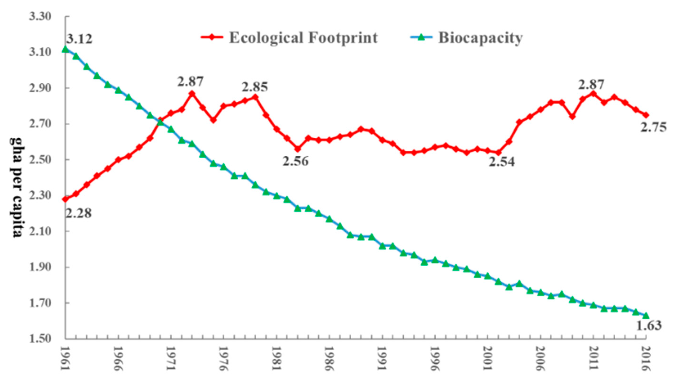
Data of the EF and BIO were obtained from the National Footprint Account results (2019 Edition) provided by Global Footprint Network (GFN). Figure 1 depicts temporal trends of the global EF and BIO from 1961 to 2016. The globally available BIO values declined continuously from 3.12 gha to 1.63 gha per capita. The global EF values increased from 2.28 gha per capita in 1961 to 2.87 gha per capita in 1973 and fluctuated between 2.54 gha and 2.87 gha per capita for the time period 1973–2016. Following 1970, the global EF values were larger than the globally available BIO values, which demonstrates that humanity’s ecological consumption exceeded the regenerative and absorptive capacities of natural capital and that humanity is living in a state of an ecological deficit.

By calculating the ratio of global EF to globally available BIO, how many Earths are needed to support humanity to be ecologically sustainable could be obtained. Figure 2 depicts evolution of the “number of Earths” needed. In 1961, 1970, 1980, 1990, 2000, 2010, and 2016, 0.73, 1.00, 1.19, 1.29, 1.38, 1.67, and 1.69 Earths were needed to support humanity to be ecologically sustainable, respectively. Before 1970, one Earth was sufficient to support humanity to be ecologically sustainable. Since 1970, we needed more than one Earth and, in general, more Earths.

As the most influential countries, the G20 countries are used as examples to illustrate national ecological consumption.

Table 1. Ecological footprint (EF) values and “number of Earths” of G20 countries for the time period 1990–2016.

	1990		2000		2010		2016
	EF	Earths	EF	Earths	EF	Earths	EF	Earths
Argentina	3.07	1.49	3.13	1.69	3.25	1.91	3.37	2.06
Australia	8.04	3.88	8.06	4.33	8.32	4.89	6.64	4.07
Brazil	2.89	1.40	3.08	1.66	3.00	1.76	2.81	1.73
Canada	8.94	4.32	9.10	4.90	8.34	4.90	7.74	4.75
China	1.53	0.74	1.92	1.03	3.36	1.98	3.62	2.22
France	5.59	2.70	5.54	2.98	5.25	3.09	4.45	2.73
Germany	6.90	3.34	5.51	2.96	5.39	3.17	4.84	2.97
India	0.78	0.38	0.86	0.46	1.07	0.63	1.17	0.72
Indonesia	1.20	0.58	1.35	0.73	1.51	0.89	1.69	1.04
Italy	5.18	2.51	5.60	3.01	5.29	3.11	4.44	2.72
Japan	5.46	2.64	5.29	2.84	4.69	2.76	4.49	2.76
Republic of Korea	3.74	1.81	5.06	2.72	5.88	3.46	6.00	3.68
Mexico	2.50	1.21	2.85	1.53	3.18	1.87	2.60	1.60
Russia	6.90	3.34	4.69	2.52	5.35	3.15	5.16	3.17
Saudi Arabia	2.13	1.03	3.77	2.03	5.66	3.33	6.23	3.83
South Africa	3.36	1.62	3.05	1.64	3.60	2.12	3.15	1.93
Turkey	2.58	1.25	2.92	1.57	3.21	1.89	3.36	2.06
United Kingdom	5.84	2.82	5.73	3.08	5.31	3.12	4.37	2.68
United States	9.87	4.77	10.25	5.52	8.94	5.26	8.10	4.97

Notes: The EF value of Russia of 1990 is not available and the data in the row is of the year 1992.

lists the EF values and “number of Earths” of the G20 countries from 1990 to 2016 (“number of Earths” is the ratio of national EF to globally available BIO, which means that, if the level of ecological consumption of one certain country is universal, this is how many Earths would be needed to support humanity to be ecologically sustainable). For the time period 1990–2016, only the EF values of India were lower than the globally available BIO, and India was the only country with an ecological surplus; China and Indonesia transformed from countries with an ecological surplus into countries with an ecological deficit; the EF values of the United States and Canada were extremely large. In 2000, the EF value of the United States was even higher than 10 gha per capita and 5.52 Earths were needed to support the lifestyle of the United States.

It is encouraging to find that the EF values of four developed countries (France, Germany, Japan, and the United Kingdom) show downward trends. The EF values of Germany decreased by the largest extent (29.84%). In 2016, the EF value of Germany was about 40% lower than the EF of the United States. The EF values of seven countries (Argentina, China, India, Indonesia, Turkey, Republic of Korea, and Saudi Arabia) show upward trends. The EF values of Republic of Korea, China, and Saudi Arabia increased by 60.63%, 136.72%, and 193.10%, respectively.

3. Influencing Factors and Control Variables

Why the four influencing factors and two control variables are selected is discussed in detail. The related and most recent literature is reviewed. In terms of the relationships between the four influencing factors and ecological consumption, four hypotheses are established.

3.1. Urbanization

As an important economic and social transformation, urbanization is treated as one of foremost influencing factors of ecological consumption. However, the impacts of urbanization on ecological consumption are controversial. On the one hand, because urbanization typically goes hand-in-hand with the industrial process, urbanization would increase ecological consumption due to more consumption of fossil fuels, construction land, cars, electric appliances, and so on. On the other hand, urbanization goes in parallel with a high population density and more ecologically oriented institutions, policies, plans, and technologies, which would permit more efficient use of ecological consumption and, thus, reduce ecological consumption.

By employing the EF as the proxy of ecological consumption and based on panel datasets, Danish and Wang confirmed a positive relationship between urbanization and ecological consumption in 11 emerging countries during 1971–2014 [19], Baloch et al. confirmed a positive relationship in 59 Belt and Road countries for the time period 1990–2016 [20], and Wang and Dong confirmed a positive relationship in 14 sub-Saharan Africa countries for the time period 1990–2014 [21].

By employing the EF as the proxy of ecological consumption, some literature confirmed a negative relationship between urbanization and ecological consumption. Based on time series datasets, Nathaniel et al. confirmed a negative relationship in South Africa for the time period 1965–2014 [22], Ahmed and Wang confirmed a negative relationship in India for the time period 1971–2014 [23], and Dogan et al. confirmed a negative relationship in Nigeria for the time period 1971–2013 [24]. Based on a panel dataset during 1990–2013, Balsalobre-Lorente et al. confirmed a negative relationship in MINT countries (Mexico, Indonesia, Nigeria, and Turkey) [25]. Based on three panel datasets for the time period 1975–2007, Charfeddine and Mrabet found that urbanization would reduce ecological consumption in 15 Middle East and North African (MENA) countries, eight oil-exporting MENA countries and seven non-oil-exporting MENA countries [26].

It is expected that the negative impacts of urbanization on ecological consumption are stronger than the positive impacts and would dominate the relationships between urbanization and ecological consumption. High-density, compact, and modern urban lifestyles are more likely to bring lower levels of ecological consumption. Therefore, the following hypothesis is established:

Hypothesis 1 (H1).

Urbanization would reduce ecological consumption.

3.2. Renewable Energy Consumption

By employing the EF to measure ecological consumption, the estimated relationship between renewable energy consumption and ecological consumption is consistent. Based on two time series datasets, Dogan et al. found a negative relationship between renewable energy consumption and ecological consumption in Nigeria and Turkey for the time period 1971–2013 [24]. Based on panel datasets, Alola et al. confirmed a negative relationship in 16 European Union (EU) countries for the time period 1997–2014 [27], Shujah-ur-Rahman et al. confirmed a negative relationship in 16 Central and Eastern European Countries for the time period 1991–2014 [28], Wang and Dong confirmed a negative relationship in 14 sub-Saharan African countries for the time period 1990–2014 [21], Balsalobre-Lorente et al. confirmed a negative relationship in the MINT countries for the time period 1990–2013 [25], and Olanipekun et al. confirmed a negative relationship in eleven Central and West African countries for the time period 1996–2015 [29].

Renewable energy consumption would reduce greenhouse gas emissions and other pollutants, which constitute major parts of ecological consumption [30,31]. Renewable energy consumption is considered as a key option for reduction in fossil-fuel consumption [32,33]. Whether the EKC hypothesis is valid or not is determined by the significance of renewable energy consumption [10], and that increasing the role of renewable energy consumption is a fundamental strategy in decreasing environmental pressures. In addition, renewable energy consumption may make individuals conscious of ecologically friendly behaviors and lifestyles. Therefore, the following hypothesis is established:

Hypothesis 2 (H2).

Renewable energy consumption would reduce ecological consumption.

3.3. Service Industries

Relative to agricultural and industrial industries, service industries are generally less material- and energy-intensive [29,34]. More importantly, service industries could improve technical efficiencies in using ecological consumption [35]. If service industries account for larger proportions of economic output, national ecological consumption is more likely to be reduced. A paradigm shift from material-intensive and energy-intensive industries to service-centered industries is urgently needed to mitigate negative impacts of ecological overshoot and crisis [36]. Therefore, the following hypothesis is established:

Hypothesis 3 (H3).

Service industries would reduce ecological consumption.

3.4. Internet Usage

Internet changes traditional ways of consumption and production and creates a new economic form, i.e., the internet economy. The internet economy has the potential to reduce ecological consumption in two ways. Firstly, the internet economy is much less material- and energy-intensive than traditional industries; secondly and more importantly, the internet economy could improve the efficiency of every sector of the economy in transforming ecological consumption into economic output [37]. In addition, the internet promotes and facilitates the collaborative economy or the sharing economy, which has the potential to reduce ecological consumption [38,39]. Therefore, the following hypothesis is established:

Hypothesis 4 (H4).

Internet usage would reduce ecological consumption.

3.5. Control Variables: Education and Income

Because education embodies a lot of information on economic and social progress such as scientific and technological progress and human capital accumulation, it is an important and essential control variable. Education may reduce ecological consumption by stimulating ecological awareness and increasing pro-ecological practices. Higher education levels would enable individuals to have more access to various scientific information and knowledge to understand complicated environmental issues and identify causes and consequences of ecological crisis [29]. Furthermore, higher levels of education would increase individual willingness to live an ecologically sustainable life such as installing more renewable energy equipment and participating more in recycling activities [23].

The negative impacts of education may be insignificant because of the attitude–behavior gap [40]. In practice, higher education levels and enough information and comprehension of the ecological crisis may not be transformed into ecologically friendly lifestyles and consumption habits. Moreover, individuals with higher levels of education tend to have high levels of living standards, which often demand higher levels of ecological consumption. Therefore, it is unclear whether education would reduce ecological consumption or not.

Because the EKC hypothesis is quite well known and the EF is a consumption-side proxy of ecological consumption, income is the most important control variable. The EKC hypothesis implies that there is an inversed U-shaped relationship between ecological consumption and income. At low levels of income, levels of ecological consumption and income tend to increase simultaneously. When income reaches a threshold point, levels of ecological consumption would decrease along with further increases in income levels.

Based on a panel dataset of 16 Central and Eastern European Countries during 1991–2014, Shujah-ur-Rahman et al. validated an N-shaped relationship between income and the EF [28]. Based on a panel dataset of 26 EU countries for the time period 1990–2013 and employing the sub-footprints of the EF as the indicators of ecological consumption, Aydin et al. revealed that the EKC hypothesis is not valid [17]. However, based on a panel dataset of 16 EU countries for the time period 1997–2014, Alola et al. found that a 1% increase in real GDP would reduce total EF by 0.81%, which supports the EKC [27]. The above literature shows that the estimations of the EKC hypothesis for developed countries are inconsistent.

By employing the EF to measure ecological consumption, estimations of the EKC hypothesis for developing countries are also inconclusive. Based on time series datasets, Ahmed and Wang confirmed the EKC in India for the time period 1971–2014 [23], and Dogan et al. confirmed the EKC in each of the MINT countries during 1971–2013 [24]. Based on panel datasets, Balsalobre-Lorente et al. validated the EKC in the MINT countries for the time period 1990–2013 [25], but Wang and Dong indicated that economic growth and ecological consumption were positively related in 14 sub-Saharan Africa countries for the time period 1990–2014 [21]. Based on three panel datasets during 1975–2007, Charfeddine and Mrabet showed that the EKC hypothesis was valid in 15 MENA countries and eight oil-exporting MENA countries, and that the relationship between economic growth and ecological consumption was U-shaped in seven non-oil-exporting MENA countries [26].

4. Regression Variables, Data Sources, and Econometric Framework

To conduct empirical estimations, “urban population (% of total population)” (URB) is employed to measure urbanization, “renewable energy consumption (% of total final energy consumption)” (REN) is employed to measure renewable energy consumption, “services, value added (% of GDP)” (SER) is employed to measure service industries, and “individuals using the internet (% of population)” (INT) is employed to measure internet usage. For the control variables, “mean years of schooling (years)” (MYS) is employed to measure education, and “gross national income per capita, PPP (current international $)” (GNIPC) is employed to measure income. Abbreviations of all of the regression variables are listed in

Table 2. List of abbreviations of the regression variables.

Abbreviation	Variable
EF	Ecological footprint
URB	Urban population (% of total population)
REN	Renewable energy consumption (% of total final energy consumption)
SER	Services, value added (% of GDP)
INT	Individuals using the internet (% of population)
MYS	Mean years of schooling
GNIPC	Gross national income per capita

.

Data of URB, REN, SER, INT, and GNIPC were obtained from the World Bank Indicators. Data of MYS were obtained from the Human Development Reports of the United Nations Development Program. All of the data used were obtained from public and reliable data sources, which could guarantee that the regression estimations are repeatable and testable.

After sorting out all of the data of the seven variables and based on the criteria of selecting the sample countries, we finally obtained three panel datasets, i.e., all sample countries (90), the developed countries (42), and the developing countries (48), for the time period 1996–2015. Lists of the developed countries and the developing countries are presented in

Table 3. List of 42 developed countries.

Developed Countries
Albania	France	North Macedonia
Australia	Germany	Norway
Austria	Greece	Poland
Belarus	Hungary	Portugal
Belgium	Ireland	Romania
Bosnia and Herzegovina	Israel	Russian Federation
Bulgaria	Italy	Serbia
Canada	Japan	Slovak Republic
Croatia	Republic of Korea	Slovenia
Cyprus	Latvia	Spain
Czech	Lithuania	Sweden
Denmark	Moldova	Switzerland
Estonia	Netherlands	United Kingdom
Finland	New Zealand	United States

and

Table 4. List of 48 developing countries.

Developing Countries
Angola	Ecuador	Niger
Argentina	Egypt	Pakistan
Bangladesh	Ethiopia	Peru
Benin	Ghana	Philippines
Bolivia	Guatemala	Rwanda
Brazil	Guinea	Senegal
Burkina Faso	Haiti	South Africa
Burundi	India	Sri Lanka
Cambodia	Indonesia	Thailand
Cameroon	Kazakhstan	Tunisia
Chad	Madagascar	Turkey
Chile	Malawi	Uganda
China	Malaysia	Venezuela
Colombia	Mali	Vietnam
Cote d’Ivoire	Mexico	Zambia
Dominican Republic	Morocco	Zimbabwe

, respectively. Statistical descriptions of the seven variables for all sample countries, the developed countries, and the developing countries are presented in

Table 5. Statistical descriptions of the variables for all sample countries (1996–2015). Obs—observations; Min—minimum; Max—maximum.

Variable	Obs	Mean	SD	Min	Max
EF	1790	3.40	2.22	0.50	10.48
URB	1800	57.13	22.22	7.41	97.88
REN	1796	33.77	29.10	0.61	98.09
SER	1786	53.12	9.86	17.99	77.02
INT	1778	27.40	28.85	0.00	96.81
MYS	1773	8.12	3.40	0.90	14.10
GNIPC	1794	14,562.42	13,688.90	450.00	68,100.00

,

Table 6. Statistical descriptions of the variables for the developed countries (1996–2015).

Variable	Obs	Mean	SD	Min	Max
EF	830	5.27	1.73	1.09	10.48
URB	840	70.41	13.27	39.47	97.88
REN	840	15.79	12.95	0.61	60.19
SER	838	59.22	7.96	35.70	76.92
INT	826	45.83	29.29	0.00	96.81
MYS	832	10.93	1.49	6.50	14.10
GNIPC	835	24,869.68	13,180.40	2180.00	68,100.00

and

Table 7. Statistical descriptions of the variables for the developing countries (1996–2015).

Variable	Obs	Mean	SD	Min	Max
EF	960	1.78	0.99	0.50	6.83
URB	960	45.50	21.97	7.41	91.50
REN	956	49.57	30.17	1.15	98.09
SER	948	47.73	8.08	17.99	77.02
INT	952	11.41	16.10	0.00	76.63
MYS	941	5.63	2.58	0.90	11.70
GNIPC	959	5587.91	5123.61	450.00	26,360.00

, respectively. Furthermore, to estimate the lagged impacts of the independent variables on the EF (lagged by one year) and have as many observations as possible, data of the EF in 2016 for all sample countries were obtained.

Based on panel datasets, the ordinary least square (OLS) was employed to conduct the estimations. We employed Equation (1) to estimate the impacts of the influencing factors and control variables on ecological consumption. Equation (2) is the specification of Equation (1).

$$EF=f(URB,REN,SER,INT,MYS,GNIPC).$$

(1)

$$\begin{array}{l}E{F}_{i,t}=\alpha +{\beta }_{1}UR{B}_{i,t}+{\beta }_{2}RE{N}_{i,t}+{\beta }_3^{}SE{R}_{i,t}+{\beta }_{4}IN{T}_{i,t}+{\beta }_{5}MY{S}_{i,t}\\ +{\beta }_{6}Ln{(GNIPC)}_{i,t}+{\beta }_{7}Ln{(GNIPC)}^2{}_{i,t}+{\epsilon }_{i,t}\end{array}$$

(2)

EF was the dependent variable and URB, REN, SER, INT, MYS, Ln(GNIPC), and Ln(GNIPC)² were the independent variables. Ln(GNIPC) is the natural log form of GNIPC. Ln(GNIPC)² is the square of Ln(GNIPC). Because marginal impacts of income on ecological consumption are supposed to be diminished, Ln(GNIPC) rather than GNIPC is used in Equation (2). Relative to GNIPC, Ln(GNIPC) could minimize the potential estimation bias caused by extreme income values. $\alpha$ represents the intercept term. ${\beta }_1,{\beta }_2,{\beta }_3,{\beta }_4,{\beta }_5,{\beta }_6$, and ${\beta }_7$ represent the slope coefficients of URB, REN, SER, INT, MYS, Ln(GNIPC), and Ln(GNIPC)², respectively. $i$ represents the sample countries (cross-section), which indicates the country-specific effects. $t$ denotes the time period (years), which indicates the time series effects. ${\epsilon }_{i,t}$ is the stochastic error term, which captures the impacts of all unobserved variables on EF.

According to the hypotheses in Section 3, ${\beta }_1,{\beta }_2,{\beta }_3$, and ${\beta }_4$ are expected to be negative. We still could not predict whether ${\beta }_5$ (the coefficient of MYS) is expected to be negative. For ecological consumption and income, there is a monotonically increasing linear relationship if ${\beta }_6>0$ and ${\beta }_7=0$, there is a monotonically decreasing linear relationship if ${\beta }_6<0$ and ${\beta }_7=0$, there is an inversed U-shaped relationship if ${\beta }_6>0$ and ${\beta }_7<0$, which validates the EKC hypothesis, and there is a U-shaped relationship if ${\beta }_6<0$ and ${\beta }_7>0$, which is contrary to the EKC hypothesis. For the inversed U-shaped or U-shaped relationship, it is easy to be calculated that the turning point values of income are exp ($-{\beta }_6/2{\beta }_7$) (the marginal impacts of Ln(GNIPC) on EF are equal to $\frac{dEF}{dLn(GNIPC)}={\beta }_6+2{\beta }_{7}Ln(GNIPC)$. At the turning points, the marginal impacts are zero, and the corresponding values of Ln(GNIPC) are $-{\beta }_6/2{\beta }_7$. Therefore, the corresponding values of GNIPC are exp ($-{\beta }_6/2{\beta }_7$)).

Because values of Ln(GNIPC) are above zero, an inversed U-shaped or U-shaped relationship between ecological consumption and income cannot be validated if ${\beta }_6=0$ and ${\beta }_7\ne 0$. Furthermore, it could not be concluded that income is not a significant influencing factor of ecological consumption if ${\beta }_6=0$ and ${\beta }_7=0$. Under the circumstances, a liner relationship rather than an inversed U-shaped or U-shaped relationship between ecological consumption and income should be explored and estimated. Therefore, we needed to revise Equation (2) and another estimation equation was proposed. The new estimation equation is as follows:

$$\begin{array}{l}E{F}_{i,t}=\alpha +{\beta }_{1}UR{B}_{i,t}+{\beta }_{2}RE{N}_{i,t}+{\beta }_3^{}SE{R}_{i,t}+{\beta }_{4}IN{T}_{i,t}+{\beta }_{5}MY{S}_{i,t}\\ +{\beta }_{6}Ln{(GNIPC)}_{i,t}+{\epsilon }_{i,t}\end{array}$$

(3)

In order to explore the lagged impacts of the independent variables on EF (lagged by one year), the following two equations were estimated:

$$\begin{array}{l}E{F}_{i,t}=\alpha +{\beta }_{1}UR{B}_{i,t-1}+{\beta }_{2}RE{N}_{i,t-1}+{\beta }_3^{}SE{R}_{i,t-1}+{\beta }_{4}IN{T}_{i,t-1}+{\beta }_{5}MY{S}_{i,t-1}\\ +{\beta }_{6}Ln{(GNIPC)}_{i,t-1}+{\beta }_{7}Ln{(GNIPC)}^2{}_{i,t-1}+{\epsilon }_{i,t-1}\end{array}$$

(4)

$$\begin{array}{l}E{F}_{i,t}=\alpha +{\beta }_{1}UR{B}_{i,t-1}+{\beta }_{2}RE{N}_{i,t-1}+{\beta }_3^{}SE{R}_{i,t-1}+{\beta }_{4}IN{T}_{i,t-1}+{\beta }_{5}MY{S}_{i,t-1}\\ +{\beta }_{6}Ln{(GNIPC)}_{i,t-1}+{\epsilon }_{i,t-1}\end{array}$$

(5)

We could present the regression results by mainly estimating Equations (2) and (4). If an inversed U-shaped or U-shaped relationship between ecological consumption and income could not be validated, Equations (3) and (5) were estimated instead to explore the linear relationship. Based on the three panel datasets, this paper follows the subsequent seven regression procedures:

• This paper estimates Equation (2) by employing the country random effects model. The estimation is called Model (1);
• This paper estimates Equation (2) by employing the country fixed effects model. The estimation is called Model (2);
• Between the country random effects model and the country fixed effects model, this paper selects an appropriate model by employing the Hausman test;
• To minimize the potential estimation bias caused by heteroscedasticity, this paper estimates Equation (2) by employing the selected appropriate model and robust standard errors. Robust standard errors are clustered on the country. The estimation is called Model (3);
• To explore the lagged impacts of the independent variables on EF (lagged by one year), this paper estimates Equation (4) by employing the selected appropriate model and robust standard errors. Robust standard errors are clustered on the country. The estimation is called Model (4);
• If there is not an inversed U-shaped or U-shaped relationship between ecological consumption and income, this paper estimates Equation (3) by employing the selected appropriate model and robust standard errors. Robust standard errors are clustered on the country. The estimation is called Model (5);
• If there is not an inversed U-shaped or U-shaped relationship between ecological consumption and lagged income (lagged by one year), this paper estimates Equation (5) by employing the selected appropriate model and robust standard errors. Robust standard errors are clustered on the country. The estimation is called Model (6).

5. Regression Estimation Results

Estimation results of the impacts of the influencing factors and control variables on ecological consumption for the three samples are presented. For all sample countries, Models (1)–(6) are presented, and Models (5) and (6) should be used to describe the impacts. For the developed countries and the developing countries, Models (1)–(4) are presented, and Models (3) and (4) should be used to describe the impacts.

5.1. All Sample Countries (90)

Estimation results of the impacts of the influencing factors and control variables on ecological consumption for all sample countries are presented in

Table 8. Estimations of impacts of influencing factors and control variables for all sample countries.

	Model (1)	Model (2)	Model (3)	Model (4)	Model (5)	Model (6)
	Coefficient (Prob.)	Coefficient (Prob.)	Coefficient (RSE)	Coefficient (RSE)	Coefficient (RSE)	Coefficient (RSE)
URB	−0.003 (0.53)	−0.033 *** (0.00)	−0.033 *** (0.01)	−0.029 ** (0.01)	−0.034 *** (0.01)	−0.030 ** (0.01)
REN	−0.028 *** (0.00)	−0.031 *** (0.00)	−0.031 *** (0.01)	−0.026 *** (0.01)	−0.027 *** (0.01)	−0.025 *** (0.01)
SER	−0.014 *** (0.00)	−0.018 *** (0.00)	−0.018 *** (0.00)	−0.018 *** (0.01)	−0.019 *** (0.01)	−0.019 *** (0.01)
INT	−0.012 *** (0.00)	−0.005 *** (0.00)	−0.005 * (0.00)	−0.005 * (0.00)	−0.002 (0.00)	−0.004 * (0.00)
MYS	0.075 *** (0.00)	0.013 (0.58)	0.013 (0.05)	0.015 (0.05)	0.001 (0.05)	0.010 (0.05)
Ln(GNIPC)	−2.958 *** (0.00)	−0.956 *** (0.01)	−0.956 (0.80)	−0.078 (0.89)	0.592 *** (0.18)	0.591 *** (0.20)
Ln(GNIPC)2	0.215 *** (0.00)	0.093 *** (0.00)	0.093 * (0.05)	0.040 (0.06)
Constant	13.858 *** (0.00)	8.228 *** (0.00)	8.228 *** (3.16)	4.353 (3.48)	2.031 (1.29)	1.673 (1.40)
Prob > F-statistic		0.00	0.00	0.00	0.00	0.00
Prob > chi2	0.00
R-squared	0.68	0.18	0.18	0.15	0.17	0.15
Obs	1728	1728	1728	1729	1728	1729
Groups	90	90	90	90	90	90

Notes: *, **, and *** denote significance at the 10%, 5%, and 1% levels, respectively; for Models (1) and (2), probability values (Prob.) are reported in parentheses; for Models (3–6), robust standard errors (RSE) are reported in parentheses.

. As can be seen from Models (1) and (2), the estimation results based on the country random effects model and the country fixed effects model were different, especially for the impacts of URB and MYS. Therefore, the Hausman test was conducted to select an appropriate model. The result of the Hausman test (the chi-square statistic was significant at the 1% level) shows that the null hypothesis, i.e., the country random effects model is appropriate, was rejected. Therefore, the country fixed effects model was selected.

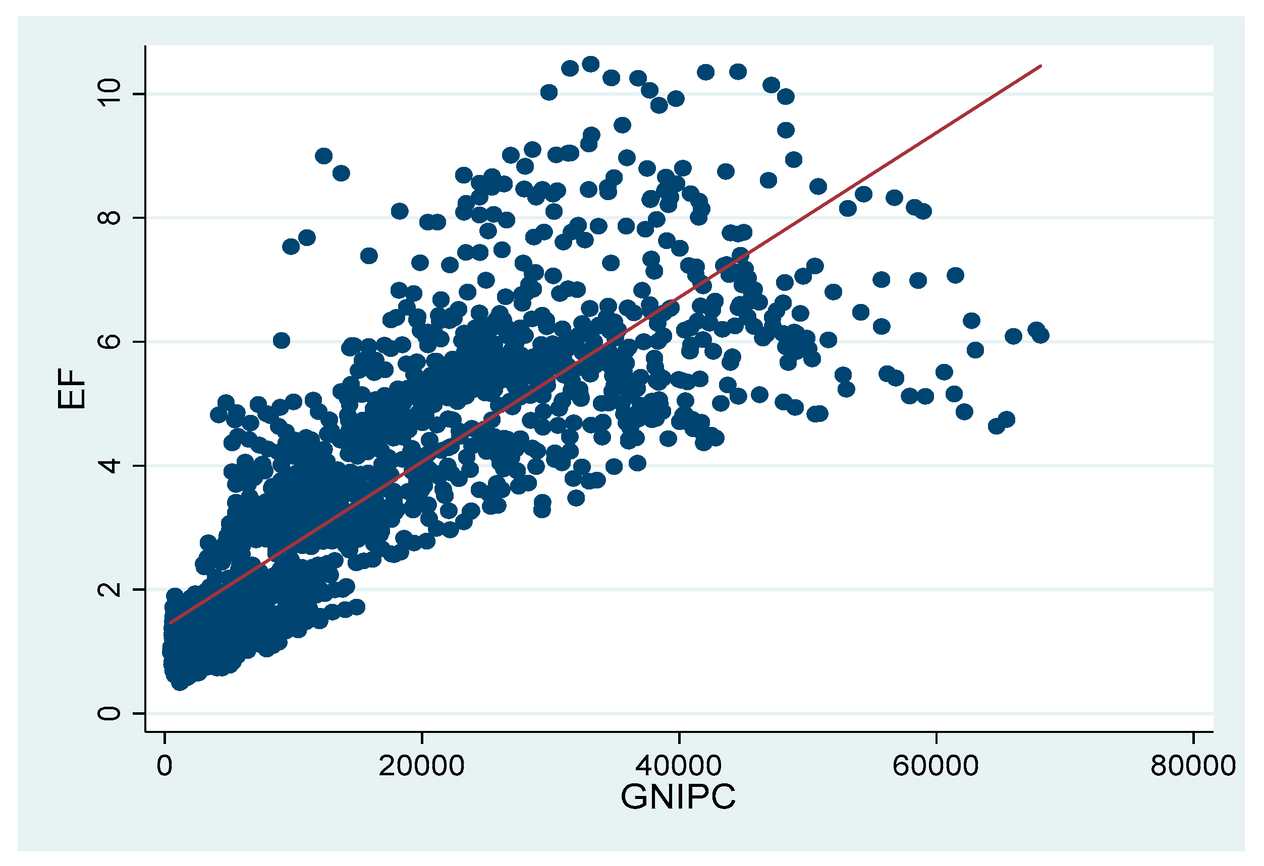
In Model (3), Ln(GNIPC) was not statistically significant. In Model (4), neither Ln(GNIPC) nor Ln(GNIPC)² was significant. According to the arguments in Section 4, an inversed U-shaped or U-shaped relationship between ecological consumption and income could not be statistically validated. Therefore, a linear relationship was explored instead. The scatter plot of EF and GNIPC (Figure 3) further demonstrates that a linear relationship was more appropriate. We ought to interpret the estimated relationships between the independent variables and EF based on the Models (5) and (6).

In Models (5) and (6), the estimated coefficients and significant extents of URB, REN, SER, MYS, and Ln(GNIPC) showed small differences. URB, REN, and SER had statistically significant and negative impacts on EF. Ln(GNIPC) had statistically significant and positive impacts on EF. MYS was statistically insignificant. The fact that INT was statistically significant in Model (6) and insignificant in Model (5) demonstrates that INT only had significant lagged impacts on EF. Relative to URB, REN, and SER, the lagged impacts of INT were weaker. The variance inflation factor (VIF) values of MYS and INT were 4.69 and 3.22, respectively, which demonstrates that the estimations of MYS and INT were not likely affected by the problems with multicollinearity.

To sum up, for all sample countries, urbanization, renewable energy consumption, and service industries were the significant influencing factors of reducing ecological consumption; internet usage only had lagged negative impacts on ecological consumption; education had no significant impacts on ecological consumption; ecological consumption and income were positively related. The relationship was linear rather than inversely U-shaped, and the EKC hypothesis was not supported.

5.2. Developed Countries (42)

Estimation results of the impacts of the influencing factors and control variables on ecological consumption for the developed countries are presented in

Table 9. Estimations of impacts of influencing factors and control variables for the developed countries.

	Model (1)	Model (2)	Model (3)	Model (4)
	Coefficient (Prob.)	Coefficient (Prob.)	Coefficient (RSE)	Coefficient (RSE)
URB	0.004 (0.64)	−0.046 *** (0.00)	−0.046 ** (0.02)	−0.046 ** (0.02)
REN	−0.051 *** (0.00)	−0.058 *** (0.00)	−0.058 *** (0.01)	−0.046 *** (0.01)
SER	−0.060 *** (0.00)	−0.077 *** (0.00)	−0.077 *** (0.01)	−0.069 *** (0.02)
INT	−0.005 *** (0.01)	0.003 (0.18)	0.003 (0.00)	0.003 (0.00)
MYS	0.122 *** (0.00)	0.119 *** (0.00)	0.119 (0.07)	0.091 (0.08)
Ln(GNIPC)	4.498 *** (0.00)	6.017 *** (0.00)	6.017 *** (2.01)	8.407 *** (2.32)
Ln(GNIPC)2	−0.188 *** (0.00)	−0.285 *** (0.00)	−0.285 ** (0.11)	−0.423 *** (0.13)
Constant	−17.801 *** (0.00)	−18.954 *** (0.00)	−18.954 ** (8.83)	−29.425 *** (10.28)
Prob > F-statistic		0.00	0.00	0.00
Prob > chi2	0.00
R-squared	0.12	0.32	0.32	0.28
Obs	810	810	810	811
Groups	42	42	42	42

Notes: *, **, and *** denote significance at the 10%, 5%, and 1% levels, respectively; for Models (1) and (2), probability values (Prob.) are reported in parentheses; for Models (3) and (4), robust standard errors (RSE) are reported in parentheses.

. As can be seen from Models (1) and (2), the estimation results based on the country random effects model and the country fixed effects model were different, especially for the impacts of URB and INT. Therefore, the Hausman test was conducted to select an appropriate model. The result of the Hausman test shows that the country fixed effects model should be selected.

In Models (3) and (4), the estimated coefficients and significant extents of URB, REN, SER, INT, MYS, Ln(GNIPC), and Ln(GNIPC)² showed small differences. URB, REN, and SER had statistically significant and negative impacts on EF. Ln(GNIPC) and Ln(GNIPC)² had significantly positive and negative impacts on EF, respectively, which validated an inversed U-shaped relationship between ecological consumption and income. 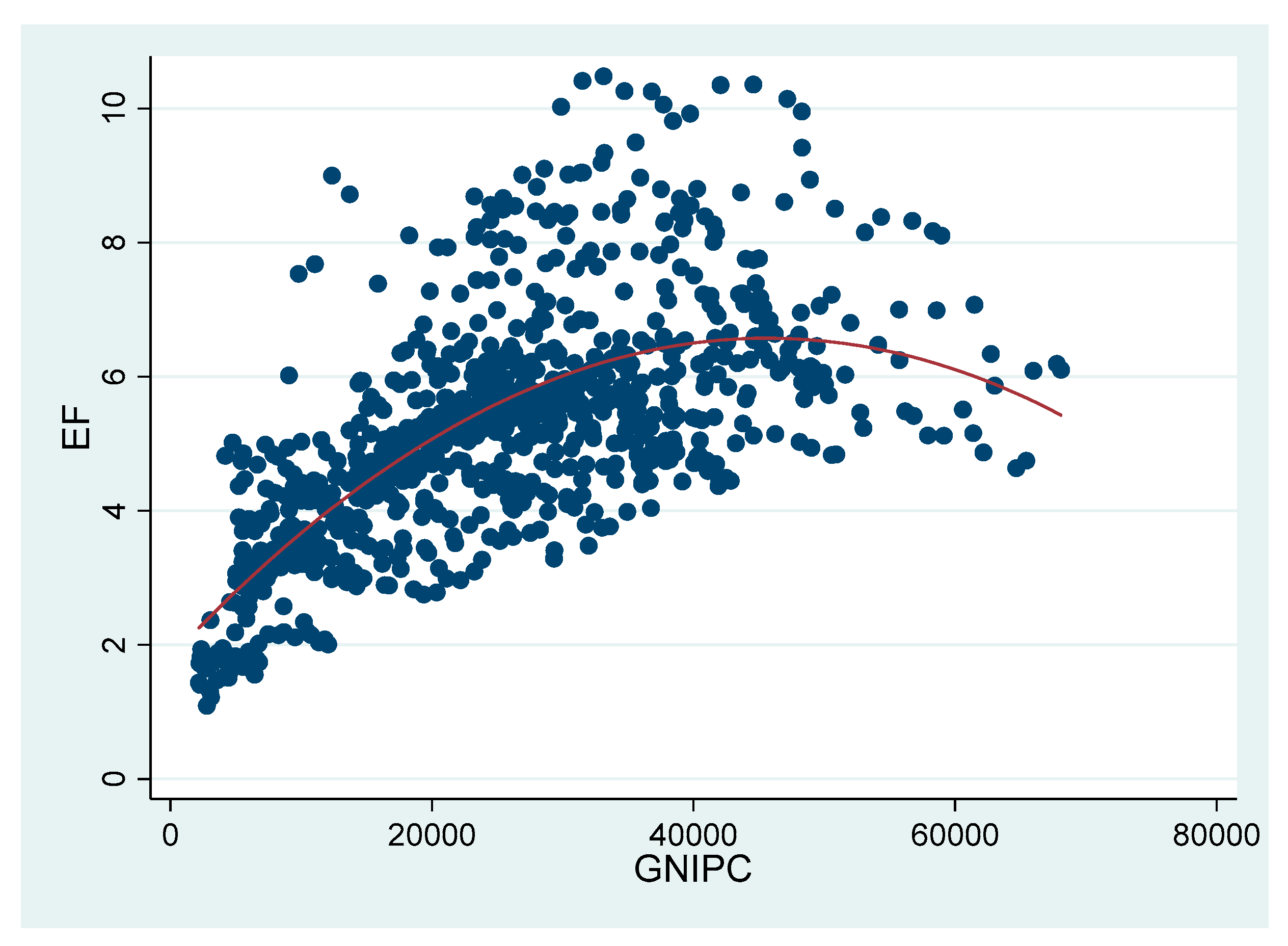According to the estimated coefficients of Ln(GNIPC) and Ln(GNIPC)² in Model (3), the turning point value of GNIPC of the inversed U-shaped relationship was 39,014. The scatter plot of EF and GNIPC (Figure 4) further verifies the turning point. For the sample, there were about 15% of the observations with GNIPC values higher than the turning point. INT and MYS were statistically insignificant. The VIF values of INT and MYS were 3.09 and 2.02, respectively, which demonstrates that the estimations of INT and MYS were not likely affected by the problems with multicollinearity.

To sum up, for the developed countries, urbanization, renewable energy consumption, and service industries were the significant influencing factors of reducing ecological consumption; internet usage and education had no significant impacts on ecological consumption; the relationship between ecological consumption and income was inversely U-shaped, and the EKC was supported.

5.3. Developing Countries (48)

Estimation results of the impacts of the influencing factors and control variables on ecological consumption for the developing countries are presented in

Table 10. Estimations of impacts of influencing factors and control variables for the developing countries.

	Model (1)	Model (2)	Model (3)	Model (4)
	Coefficient (Prob.)	Coefficient (Prob.)	Coefficient (RSE)	Coefficient (RSE)
URB	−0.005 * (0.08)	−0.014 *** (0.00)	-0.014 (0.01)	−0.014 (0.01)
REN	−0.008 *** (0.00)	−0.008 *** (0.00)	−0.008 ** (0.00)	−0.006 * (0.00)
SER	−0.004 ** (0.02)	−0.004 ** (0.02)	−0.004 * (0.00)	−0.006 ** (0.00)
INT	−0.005 *** (0.00)	−0.004 *** (0.00)	−0.004 * (0.00)	−0.006 * (0.00)
MYS	−0.042 ** (0.02)	−0.061 *** (0.00)	−0.061 (0.06)	−0.042 (0.04)
Ln(GNIPC)	−3.090 *** (0.00)	−2.759 *** (0.00)	−2.759 *** (0.91)	−2.941 *** (1.13)
Ln(GNIPC)2	0.228 *** (0.00)	0.210 *** (0.00)	0.210 *** (0.07)	0.225 *** (0.09)
Constant	12.724 *** (0.00)	11.683 *** (0.00)	11.683 *** (3.31)	12.137 *** (4.01)
Prob > F-statistic		0.00	0.00	0.00
Prob > chi2	0.00
R-squared	0.63	0.39	0.39	0.39
Obs	918	918	918	918
Groups	48	48	48	48

Notes: *, **, and *** denote significance at the 10%, 5%, and 1% levels, respectively; for Models (1) and (2), probability values (Prob.) are reported in parentheses; for Models (3) and (4), robust standard errors (RSE) are reported in parentheses.

. As can be seen from Models (1) and (2), the estimation results based on the country random effects model and the country fixed effects model showed some differences. The Hausman test was conducted to select an appropriate model. The result of the Hausman Test shows that the country fixed effects model was more appropriate and should be selected.

In Models (3) and (4), the estimated coefficients and significant extents of URB, REN, SER, INT, MYS, Ln(GNIPC), and Ln(GNIPC)² showed small differences. REN, SER, and INT had statistically significant and negative impacts on EF. Ln(GNIPC) and Ln(GNIPC)² had significantly negative and positive impacts on EF, respectively, which validated a U-shaped relationship between ecological consumption and income. 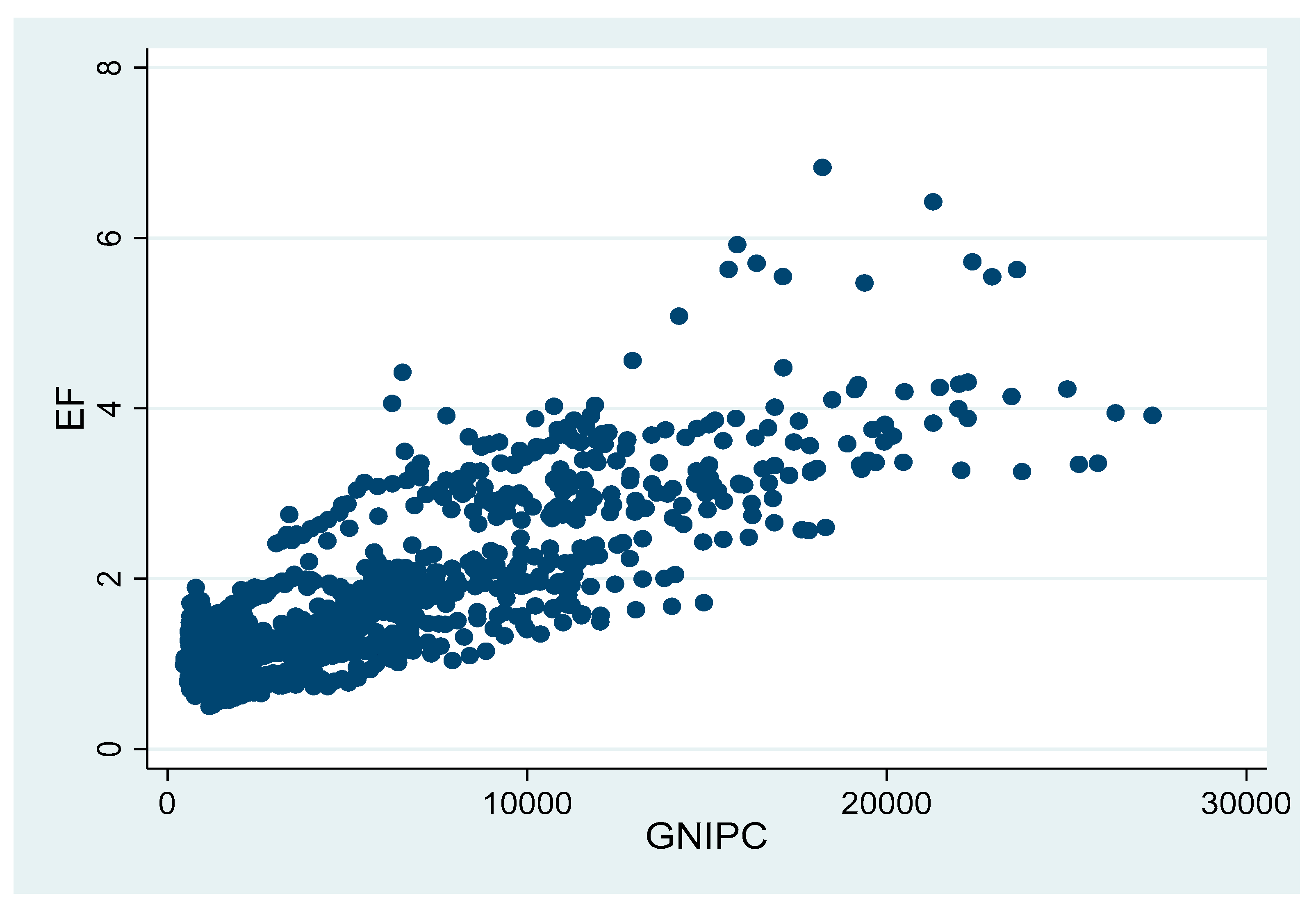According to the estimated coefficients of Ln(GNIPC) and Ln(GNIPC)² in Model (3), the turning point value of GNIPC of the U-shaped relationship was 706. The scatter plot of EF and GNIPC (Figure 5) further certifies the U-shaped relationship and the turning point. For the sample, there were about 95% of the observations with GNIPC values higher than the turning point. URB and MYS were statistically insignificant. The VIF values of URB and MYS were 3.24 and 2.82, respectively, which demonstrates that the estimations of URB and MYS were not likely affected by the problems with multicollinearity.

To sum up, for the developing countries, renewable energy consumption, service industries, and internet usage were the significant influencing factors of reducing ecological consumption; urbanization and education had no significant impacts on ecological consumption; the relationship between ecological consumption and income was U-shaped, and the EKC hypothesis was not supported.

6. Discussion and Conclusions

Humanity as a whole is living with an ecological deficit, which is widening in general. Reducing ecological consumption is a basic prerequisite and necessary condition of achieving global ecological sustainability. More and more literature explored the influencing factors of ecological consumption from multiple research perspectives. Based on three panel datasets for the time period 1996–2015, this paper adds to the literature by exploring the impacts of urbanization, renewable energy consumption, service industries, and internet usage on ecological consumption and taking education and income as the control variables.

The main contributions of this paper are as follows: (1) this paper employed the EF as the indicator of ecological consumption. The EF tracks ecological consumption in dimensions of both sources and sinks from the consumption side, which enlarges the discussion on ecological sustainability beyond a certain specific domain and is more illuminating for the demand-side policymaking; (2) by selecting representative sample countries covering all of the world, this paper estimated the impacts of the influencing factors on ecological consumption at the global level, which is helpful of summarizing universal laws of reducing ecological consumption; (3) this paper divided all 90 sample countries into 42 developed countries and 48 developing countries and found the different impacts of the influencing factors for the developed countries and the developing countries, especially the different impacts of urbanization and internet usage.

Urbanization would reduce ecological consumption in all sample countries and the developed countries. However, urbanization was not an independent and significant influencing factor of ecological consumption in the developing countries. Based on a panel dataset for the time period 1980–2015, Adams and Acheampong also demonstrated that urbanization had indeterminate and insignificant impacts on carbon emissions in 46 sub-Saharan Africa countries [30]. As discussed in Section 3.1, the negative impacts do not dominate the potential relationships between urbanization and ecological consumption in the developing countries. To further strengthen the negative impacts and weaken the positive impacts of urbanization on ecological consumption, the urban areas should be more ecologically planed (more vertical and compact rather than horizontal and sprawled), and the urban residents ought to have easier and more convenient access to ecologically efficient technologies and public infrastructure such as consumer durables and mass transit. Unplanned, scattered, and disordered urban sprawl in developing countries must be controlled through joint governance at various levels and by different public departments [41].

For all three samples, renewable energy consumption and service industries would reduce ecological consumption. Developing new, reliable, and affordable green and clean technologies to further promote renewable energy consumption and accelerating economic structure transition (less agricultural and industrial industries and more service industries) are useful and effective ways of reducing ecological consumption. By comparing Table 9 and Table 10, it could be found that the negative impacts of both renewable energy consumption and service industries in the developed countries were much stronger than those in the developing countries. The much stronger negative impacts could help explain the inversed U-shaped and U-shaped relationships between ecological consumption and income in the developed countries and the developing countries, respectively [10].

Internet usage was an independent and significant force of reducing ecological consumption in the developing countries. Internet not only brings new information, knowledge, technologies, and goods and services markets, but also more ecologically sustainable lifestyles. However, internet usage was not a significant influencing factor of ecological consumption in the developed countries. By employing the same proxy of internet usage and based on a panel dataset, Salahuddin et al. also found that internet usage could not reduce CO₂ emissions in 31 OECD (Organization for Economic Cooperation and Development) countries for the time period 1991–2012 [42]. Therefore, “internet for ecological sustainability” should be a new guidance principle when developed countries design internet businesses and industries.

Education was not an independent and significant influencing factor of ecological consumption for all three samples. The attitude–behavior gap still exists and prevents ecological awareness from being turned into real and specific ecologically friendly actions. The estimated results remind us that the ecological education we need in the “full world” and Anthropocene does not only have to do with “knowing” but also with “doing”. It is hoped that individuals with higher education levels would become the pioneers on living and promoting ecologically sustainable lives.

By employing income as the most important control variable, this paper enriches the long-lasting discussions on the EKC hypothesis and validates three kinds of relationships between ecological consumption and income. For all sample countries, income was a significant factor of increasing ecological consumption, and higher income was not the solution to ecological degradation. For the developing countries, the turning point value of GNIPC of the U-shaped curve was 706, and 95% of the observations were on the right side of the U-shaped curve, which means that, after a very early development stage, ecological consumption began increasing along with further increases in income levels. To our delight, the EKC hypothesis was valid in the developed countries. A positive relationship between ecological consumption and income was significantly reversed when GNIPC values approximately reached 39,014. For the developed countries, because only 15% of the observations were on the right side of the inversed U-shaped curve, more timely and effective measures should be taken to decouple income from ecological consumption and accelerate the arrival of the turning point of the inversed U-shaped curve, which would stimulate developing countries to make corresponding changes and help reduce global ecological consumption by much larger extents.

Much more work needs to be conducted to improve our empirical analysis and further deepen the research context. Because the variables in this paper are defined generally, future research should explore different definitions of the variables, which would give us different perspectives of exploring the influencing factors of ecological consumption. The data quality should also be improved. For example, cultural differences may affect the uniformity of the data in different countries, especially in developed and developing countries. A major drawback of the regression estimations is that we did not find instrumental variables of the influencing factors, especially the instrumental variables of urbanization and internet usage, to conduct sensitivity analyses of the estimation results. Although panel regressions were used to conduct the estimations and lagged impacts were estimated to serve as robust checks for the regression results, the causal relationships between the influencing factors and ecological consumption could not be validated. Additionally, because the regression estimations were on a global level, it was difficult to provide specific measures to reduce ecological consumption of individual countries. Future research can try to combine estimations of global and national levels.

More control variables, for example, political institutional quality and inequality, could be included in the panel regressions in order to refine the estimations. More importantly, the estimated results need further explanation. For example, why the negative impacts of renewable energy consumption and service industries are much stronger in developed countries than in developing countries needs to be explored. The reasons and evidence would provide more specific and scientific policy advice with regard to reducing ecological consumption. Finally, to have an ecologically sustainable future, humanity also has to find solutions to reverse the downward trend of globally available BIO and improve global ecological capacity, which provides more research directions in the field of ecological sustainability.