Article

Receding-Horizon Vision Guidance with Smooth Trajectory Blending in the Field of View of Mobile Robots

1
College of Mechanical and Electrical Engineering, Nanjing University of Aeronautics and Astronautics, Nanjing 210016, China
2
Department of Mechanical Engineering and Centre for Intelligent Machines, McGill University, Montreal, QC H3A 0C3, Canada
3
Department of Mechanical Engineering, Memorial University of Newfoundland, St. John’s, NL A1B 3X5, Canada
*
Author to whom correspondence should be addressed.
Appl. Sci. 2020, 10(2), 676; https://doi.org/10.3390/app10020676
Submission received: 15 November 2019 / Revised: 3 January 2020 / Accepted: 13 January 2020 / Published: 18 January 2020
(This article belongs to the Special Issue Intelligent Robotics)

Abstract

:
Applying computer vision to mobile robot navigation has been studied for over two decades. One of the most challenging problems for a vision-based mobile robot involves accurately and stably tracking a guide path in the robot limited field of view under high-speed manoeuvres. Pure pursuit controllers are a prevalent class of path tracking algorithms for mobile robots, while their performance is rather limited to relatively low speeds. In order to cope with the demands of high-speed manoeuvres, a multi-loop receding-horizon control framework, including path tracking, robot control, and drive control, is proposed in this paper. This is done within the vision guidance of differential-driving wheeled mobile robots (DWMRs). Lamé curves are used to synthesize a trajectory with G 2 -continuity in the field of view of the mobile robot for path tracking, from its current posture towards the guide path. The platform twist—point velocity and angular velocity—is calculated according to the curvature of the Lamé-curve trajectory, then transformed into actuated joint rates by means of the inverse-kinematics model; finally, the motor torques needed by the driving wheels are obtained based on the inverse-dynamics model. The whole multi-loop control process, initiated from Lamé-curve blending to computational torque control, is conducted iteratively by means of receding-horizon guidance to robustly drive the mobile robot manoeuvring close to the guide path. The results of numerical simulation show the effectiveness of our approach.

1. Introduction

Mobility is a distinct characteristic separating mobile robots from their base-fixed counterparts [1]. Navigation is an essential issue to realize the motion of mobile robots, which brings about three basic questions: (a) where am I? (b) where am I heading for? and (c) how do I get there? The third question pertains to path-guidance control [2]. If the position reference is not available temporarily, the navigation system typically enters a mode known as dead reckoning to maintain an estimate of the position [3]. Otherwies guidance involves obtaining a trajectory for a mobile robot from its position and orientation in order to follow a given path [4].
Given paths, or guide paths, the target to be continuously followed by mobile robots can be generated in various possible ways: path planning on a map (environment model) [2,5,6]; a parametric reference in a fixed coordinate frame [7,8,9,10,11]; and a physical landmark (wire, tape, stripe) on the ground [12,13,14,15]. Recently, computer vision has been used to measure the posture of mobile robots when tracking guide pathways. One approach resorts to a ceiling-mounted camera overlooking a mobile robot with specific colored labels on its platform [16,17,18]; another approach relies on an onboard camera looking down at a physical pathway (colored stripe) on the ground from the perspective of the robot [12,14,15].
For the first approach, the stationary cameras fixed in the environment have a large field of view, but at the cost of measurement precision. For example, a high-resolution camera overhead provides a positioning measurement value with a resolution of 14.9 mm for a robot with dimensions of 365 × 419 mm [17]. In this sense, cameras mounted on robots in the second approach are preferred for applications requiring a high accuracy.
Line tracking via an onboard camera is perhaps the prospective vision navigation approach mostly used in industrial environments, since it offers real-time, precise and reliable performance. The computational load relevant to this kind of vision perception is mitigated by coding or learning the specific perceptual knowledge that is expected to extract from the environment [15,19,20,21]. Moreover, gluing colored stripes on the floor is inexpensive, compared not only with laying down a wire under the ground, but also with setting up a plurality of retro reflectors for a laser guidance system [22].
However, the limited field of view of onboard cameras brings great difficulties to the path tracking of differential-driving wheeled mobile robots (DWMRs) in high-speed manoeuvres, especially when only kinematic models [12,14,17] or pure pursuit controllers [23,24,25] are used. In order to cope with the demands of high-speed manoeuvres, dynamic models are used to describe the inherent characteristics of correlating actuation with motion in a DWMR. These models are normally force-driven, second-order differential equations relating wheel forces to robot acceleration [13,18,26]. When motor dynamics is included, robot models evolve to composite models. In these models, the platform twist (A vector array that includes point velocity and rigid-body angular velocity.) can be associated with the time-derivative of motor-armature voltage [8], or with the duty ratio of pulse-width modulation (PWM) of motor voltage [27], or even with the motor current [28].
Controller design is influenced by system models of mobile robots. Pure pursuit controllers are a prevalent class of path tracking algorithms for mobile robots, while their performance is rather limited to relatively low speeds. Hence, the receding-horizon strategy is used to develop a model-based predictive active yaw control implementation for pure-pursuit tracking at high speeds [25]. The strategy is a model-based feedback control solution in terms of the limited sampling and control period, in which an optimal control trajectory is generated for the initial state, and updated at each sampled instant. This strategy can be combined with a sequential convex programming method to develop a closed-loop guidance control scheme that robustly drives a spacecraft maneuvering close to the target [29]. This strategy can also be used to control mobile robots to locate sensor nodes in unknown wireless sensor networks [30]. The strategy has proven to be effective to enhance the scheme quality and reduce the computational burden by dividing the optimization horizon into smaller time windows [31].
The underlying motivation of this paper lies in the need for combining the receding-horizon strategy with Lamé-curve blending for vision guidance in the limited field of view of mobile robots. Our main contribution is twofold. On the one hand, a multi-loop receding-horizon control framework is outlined for vision guidance of mobile robots. Herein, cascaded control loops of path tracking, robot control and drive control are developed based on kinematics and dynamics models. On the other hand, Lamé-curve blending is proposed for kinematic path tracking to generate a trajectory with G 2 -continuity to blend its current posture with a certain point of the guide path.
The balance of the paper is organized as follows: the problem description and the receding-horizon control framework for vision guidance of mobile robots are addressed in Section 2; the kinematics and dynamics models are formulated for DWMRs in Section 3; the kinematic path tracking technique based on Lamé-curve blending is proposed in Section 4; simulation results are reported in Section 5, while conclusions and recommendations for future research work are given in Section 6.

2. Problem Formulation

2.1. Vision Guidance

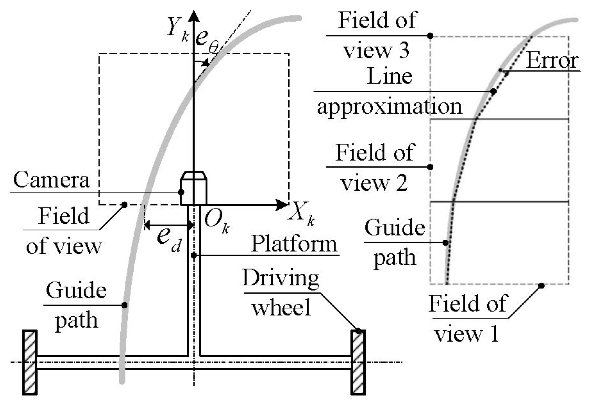
The problem under study consists in guiding a DWMR through a given path by means of a vision guidance system. An onboard camera is assumed to be mounted on the front of the DWMR, looking down obliquely at colored stripes on the ground, as shown in Figure 1.
Colored stripes in the robot field of view are recognized as guide paths. A position error e d and an orientation error e θ of the DWMR are defined with respect to a guide path, as shown in Figure 2. Moreover, e d denotes the x-coordinate of the intersection of the guide path with the X k -axis, e θ referring to the angular error between the tangent of the guide path and the Y k -axis. Fields of view 1, 2 and 3 in Figure 2 represent a sequence of vision samplings at three consecutive instants, as the robot moves. Since the field of view is relatively small, namely, 0.4 × 0.3 m, a guide path can be approximated as a straight line by means of least squares. The linearization error increases with a decrease in the radius of curvature, as shown in Table 1.
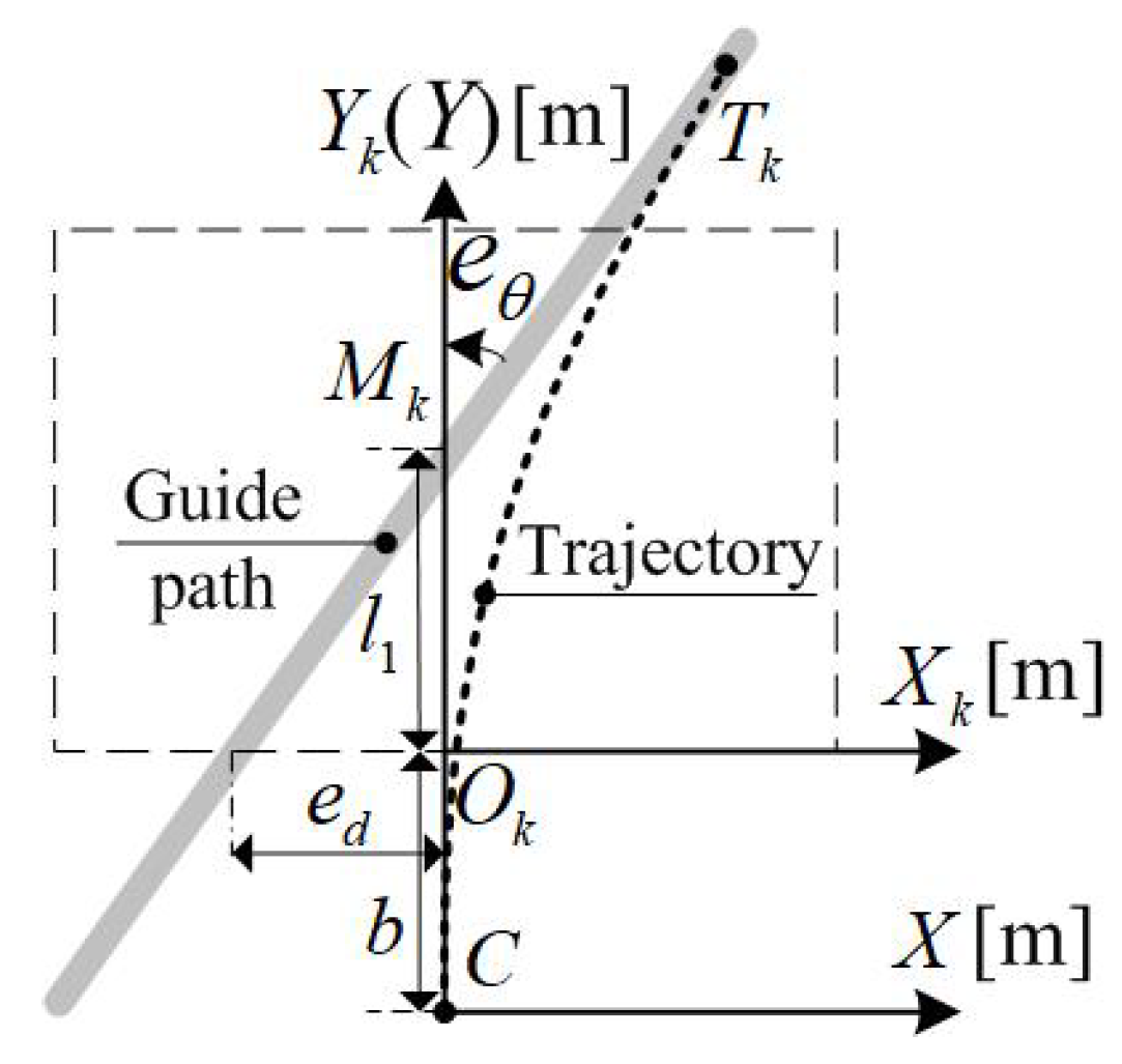
When high-curvature arcs are used for guide paths, the tangents of their different sections undergo a significant change in the field of view. In these cases, an approximation method based on binary-tree guidance window partition can be used to replace the curve with a series of piecewise lines at any given approximation accuracy [32]. Hence, only straight paths are considered as the target of tracking control in the field of view, as shown in Figure 3.
In Figure 3, point C, the centre of mass of the platform, indicates the position of the DWMR, while the angle e θ defines its orientation error with respect to the path. Path tracking can be converted into a trajectory-planning problem from the current pose (point C along the Y-axis) to a target pose (point T k along the path). It is noteworthy that path is distinguished from trajectory here. The former is the colored stripe marked on the floor, which serves to guide the robot; the latter is the curve traced by a reference point of the platform. We choose this point at the platform centre of mass.

2.2. Methodology Overview

Electric motors are the actuators of choice in most mobile robots. A typical motion control system includes a feedback subsystem with three cascaded loops: the outer position loop; the intermediate velocity loop; and the inner current loop. Nowadays, many commercial off-the-shelf motor drives provide the complete control capability for all three loops. Dynamic path-tracking can be implemented by interfacing the torque output of the inverse-dynamics model with the current-loop control of the motor drives, in a hierarchical control framework based on kinematics and dynamics models, as shown in Figure 4.
This control framework combines vision detection with cascaded control loops of path tracking, robot control and drive control, meanwhile facilitating the integration of kinematics and dynamics models with commercial off-the-shelf motor drives. First, colored stripes on the ground are recognized as guide paths, and then robot posture errors are obtained by vision detection, the errors being the vision input. Second, path tracking is used to eliminate these errors by controlling the robot twist, as the first-layer output. Third, the inverse-kinematics model transforms the twist into the actuated joint-rate vector, as the second-layer output. Fourth, the desired torque is calculated from the inverse-dynamics model for the motor drives, as the third-layer output. Finally, torque control is automatically implemented in the current loop by motor drives, which drive the mobile robot manoeuvring close to the guide path.
In this control framework, the path recognition approach based on vision detection can be found in a previous paper [32], while joint rate and torque instructions are not difficult to obtain if kinematics and dynamics models are both available. In this sense, the key issue in our vision guidance study is how to drive the mobile robot from the current pose to a target pose. Lamé-curve blending is proposed for kinematic path tracking in the field of view by means of a receding-horizon model.
The receding-horizon strategy is implemented as explained next. In each sampling period, the path image is updated by the vision guidance system as the initial state of path tracking, as shown in Figure 3. In each control period, the Lamé-curve blending technique is used to plan a trajectory with G 2 -continuity to approach the guide path. In general, several control periods may be needed to complete the process of trajectory tracking. However, only the current robot twist, determined by the trajectory curvature, is used as the control output to the inverse-kinematics model of the robot at the current instant. When the next control period comes, a new Lamé trajectory is generated according to the corresponding new path image, thereby determining a new robot twist as the next control output.
Apparently, the receding-horizon strategy can mitigate the deviations of the actual motion of mobile robots from the predefined trajectory, thereby facilitating the implementation of the kinematics path tracking in the closed-loop vision guidance framework. The sections below focus on both the kinematics and dynamics models of a DWMR, and the kinematic path tracking approach based on Lamé-curve blending.

3. Mobile Robot Modeling

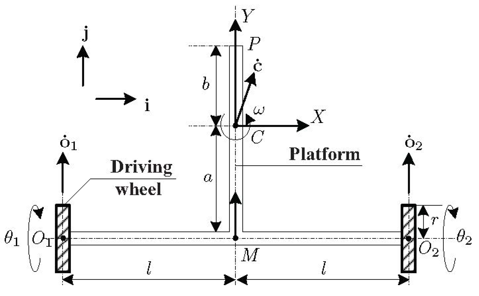
As shown in Figure 5, the platform of a DWMR is depicted as a T-shaped rigid body. Two coaxial wheels are coupled to the platform by means of revolutes of axes passing through points O 1 and O 2 . Let C be the centre of mass of the platform. Point M is the midpoint of segment O 1 O 2 ¯ . Moreover, let the position vectors of C, M, O 1 and O 2 in an inertial frame be denoted by c , m , o 1 and o 2 , respectively. Additionally, let ω be the scalar angular velocity of the platform about a vertical axis. In order to proceed with the kinematic analysis of this system, we define a moving frame F , of axes X , Y , Z , attached to the platform, with Z pointing in the upward vertical direction. Unit vectors i , j , k are defined parallel to the X-, Y-, Z-axes, respectively.

3.1. Kinematics

Let the radius of the actuated wheels be r, their angular displacements being θ 1 and θ 2 . The velocity o ˙ i of point O i , under pure-rolling, for i = 1 , 2 , is given by
o ˙ i = r θ ˙ i j i = 1 , 2
Furthermore, the velocity of C can now be expressed in two-dimensional form as
c ˙ = o ˙ i + ω E ( c o i ) , i = 1 , 2
where E is defined as an orthogonal matrix rotating two-dimensional vectors through an angle of 90 counterclockwise [33], i.e.,
E 0 1 1 0
Let the distance between the two actuated wheels be 2 l . Substituting Equation (1) into Equation (2) and subtracting sidewise the latter from the former, we obtain
r ( θ ˙ 1 θ ˙ 2 ) + 2 ω l = 0
Hence, the scalar angular velocity of the platform is derived from Equation (3) as
ω = r 2 l ( θ ˙ 2 θ ˙ 1 )
The angular velocities of the two actuated wheels are, therefore,
ω 1 = θ ˙ 1 i + ω k = i ( r / 2 l ) k ( r / 2 l ) k θ ˙ ω 2 = θ ˙ 2 i + ω k = ( r / 2 l ) k i + ( r / 2 l ) k θ ˙
with the two-dimensional vector θ ˙ of actuated joint rates defined as
θ ˙ θ ˙ 1 θ ˙ 2
Point P is defined at the front of the platform. Let the distance between C and M be a, that between C and P being b. The velocity c ˙ of point C can be obtained in terms of θ ˙ 1 and θ ˙ 2 as well, upon substitution of Equation (1) into Equation (2), and addition of Equation (2) for i = 1 to its counterpart for i = 2 , thus obtaining
c ˙ = a r 2 l ( θ ˙ 1 θ ˙ 2 ) i + r 2 ( θ ˙ 1 + θ ˙ 2 ) j
Further, the planar twist t of the platform is defined as a three-dimensional array:
t ω c ˙
the forward kinematics model of the platform then being expressed as
t = T θ ˙
with the 3 × 2 matrix T defined as
T r / ( 2 l ) r / ( 2 l ) ( a r / 2 l ) i + ( r / 2 ) j ( a r / 2 l ) i + ( r / 2 ) j
In order to derive the inverse kinematics of the platform, both sides of Equation (7) are dot-multiplied by j , thereby obtaining
c ˙ T j = r 2 ( θ ˙ 1 + θ ˙ 2 )
The scalar equations of the inverse kinematics are readily derived by combining Equations (4) and (9), namely,
θ ˙ 1 = v c r l r ω , θ ˙ 2 = v c r + l r ω
where the longitudinal speed is v c c ˙ T j , the speed of the centre of mass.

3.2. Dynamics

Within the Newton-Euler formulation applied to multibody systems, we distinguish three rigid bodies composing the DWMR, as shown in Figure 5. The 6 × 6 inertia dyad of the two actuated wheels are denoted by M 1 and M 2 , with a similar notation for their six-dimensional twists. Since the platform undergoes planar motion, its 3 × 3 counterpart inertia dyad M 3 is introduced here, while the platform twist becomes, correspondingly, the three-dimensional vector t 3 . Besides, the transformation matrices of the three moving bodies are expressed in a similar way. These relate the body twists with the vector of actuated joint rates θ ˙ , introduced in Equation (6), i.e.,
t i = T i θ ˙ , i = 1 , 2
and
t 3 = T 3 θ ˙
where, from Equations (1), (5) and (8), and considering that the two wheels undergo general six-degree-of -freedom motion,
T 1 = i r / ( 2 l ) k r / ( 2 l ) k r j 0 , T 2 = r / ( 2 l ) k i + r / ( 2 l ) k 0 r j , T 3 = r 2 1 / l 1 / l ( a / l ) i + j ( a / l ) i + j
By means of the natural orthogonal complement [34], the generalized dynamics model is derived from the Newton-Euler equations for the DWMR, which leads to
I θ ¨ = C θ ˙ + τ + δ + γ
where I is the positive definite 2 × 2 generalized inertia matrix, C θ ˙ being the 2-dimensional vector of Coriolis and centrifugal-force terms. Furthermore, τ , δ and γ denote the 2-dimensional vectors of generalized active, dissipative, and gravity forces, respectively. Moreover, the twist t is a linear transformation of the independent generalized speeds θ ˙ , as per Equation (8).
The 2 × 2 generalized inertia matrix I is obtained as
I = I w + I p = i = 1 2 T i T M i T i + ( T 3 ) T M 3 T 3
where I w and I p are the inertia matrices of the two actuated wheels and of the platform, respectively.
The 2 × 2 matrix C of Coriolis and centrifugal force is derived below:
C = i = 1 2 T i T M i T ˙ i + ( T 3 ) T M 3 T ˙ 3 + i = 1 2 T i T W i M i T i + ( T 3 ) T W 3 M 3 T 3
where W i , for i = 1 , 2 , and W 3 are, correspondingly, 6 × 6 and 3 × 3 angular-velocity dyads, defined as
M i I i O 3 O 3 m i 1 3 , W i Ω i O 3 O 3 O 3 , W 3 ω 3 0 2 T 0 2 O 2
with I i and m i denoting the 3 × 3 moment-of-inertia matrix and the mass of the ith body, while Ω i is the 3 × 3 angular velocity matrix, the cross-product matrix of the angular velocity vector ω i , i.e., Ω i = CPM ( ω i ) , defined such that for any r R 3 , ω i × r = Ω i r . Besides, O 3 , O 2 , 0 2 and 1 3 are the 3 × 3 and 2 × 2 zero matrices, the two-dimensional zero vector, and the 3 × 3 identity matrix, respectively.
In order to expand the foregoing matrices, we let I x , I y and I z be the three principal moments of inertia of the two actuated wheels, respectively. Moreover, I 3 denotes the principal moment of inertia of the platform at its centre of mass. Therefore,
I 1 = I 2 = I x 0 0 0 I y 0 0 0 I z , M 3 = I 3 0 2 T 0 2 m 3 1 2
where, 1 2 is the 2 × 2 identity matrix; because of wheel symmetry, I x = I y .
Substitution of Equations (13) and (17) into Equation (15) leads to
I w = H 1 H 2 H 2 H 1 , I p = H 3 H 3 H 3 H 3
where H i , for i = 1 , 2 , 3 , is given below:
H 1 = I x + 1 2 r l 2 I z + m 1 r 2 , H 2 = 1 2 r l 2 I z , H 3 = r 2 l 2 ( I 3 + m 3 a 2 )
The coefficient matrix C is expanded in a similar way. Since the inertia dyad M i and the angular-velocity dyad W i are block-diagonal matrices, the triad { i , j , k } will not appear in matrices T i T M i T i , T i T M i T ˙ i and T i T W i M i T i . Consequently, when the time-history of the actuated joint rates is given, the torque requirements at the different actuated joints can be determined.

4. Path Tracking

4.1. Tracking Target

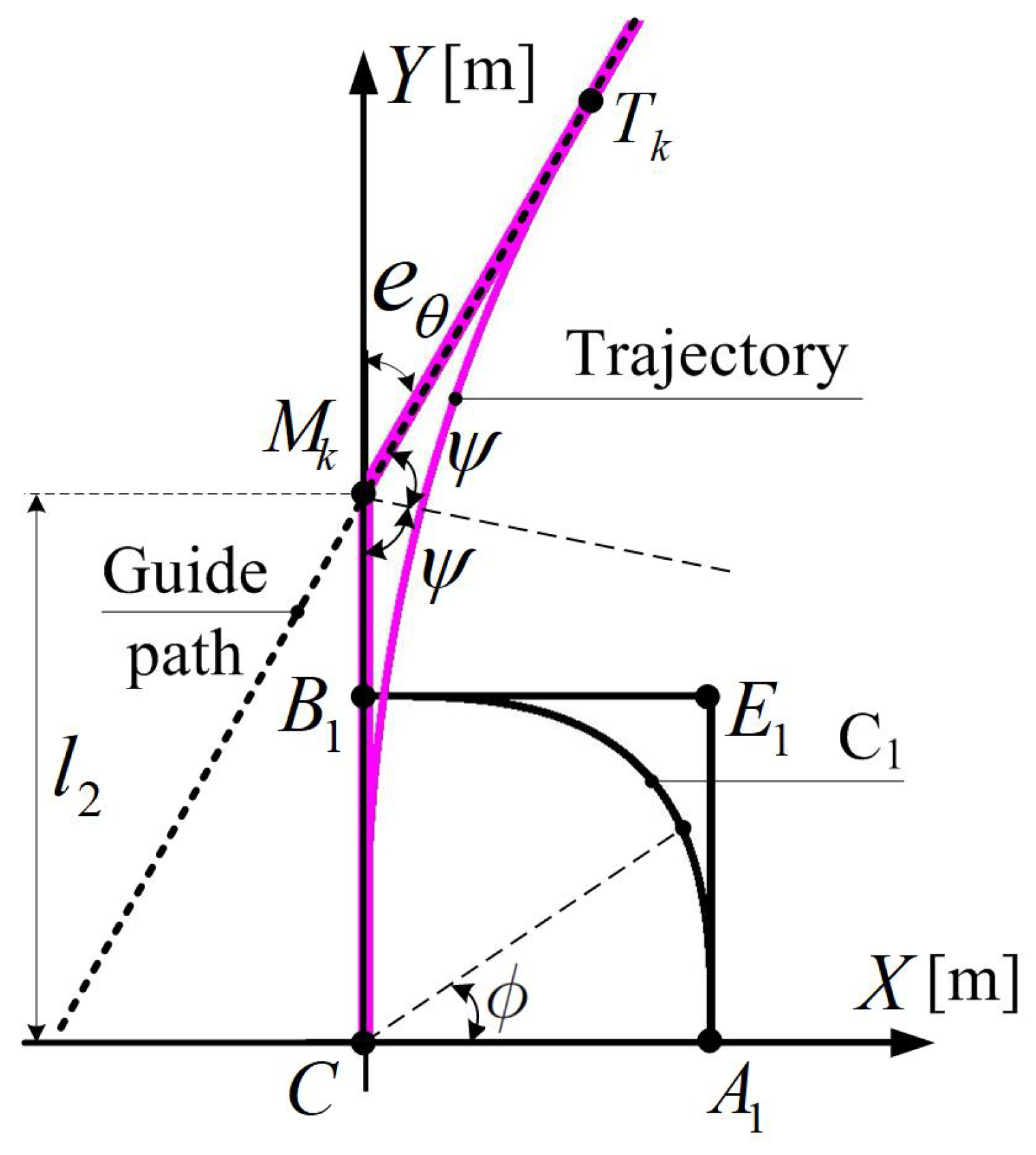
As shown in Figure 3, kinematic path tracking can be regarded as the generation of a trajectory for the mobile robot to travel along, from its current pose to the target pose. Several types of curves can be used here to blend the trajectory with the Y-axis at points C and T k of Figure 3. Compared with circular arcs and ellipses, Lamé curves can provide the full trajectory with G 2 -continuity, meaning that position, tangent and curvature are all continuous along the trajectory, including the blending points.
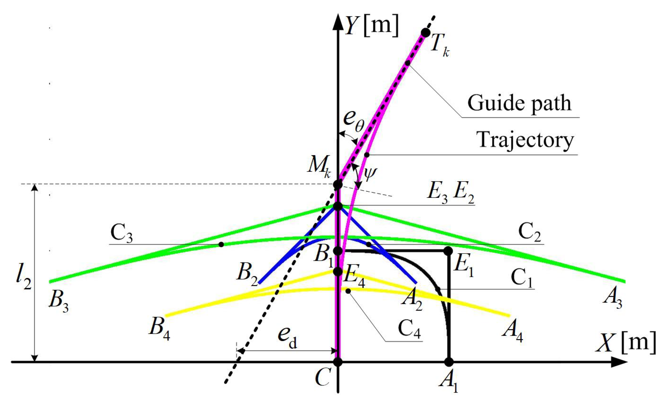
As shown in Figure 6, the trajectory, on which a robot moves toward the target pose on the prescribed path, can be obtained by curve transformation. C 1 is a standard Lamé curve, intersecting the X- and Y-axes at points A 1 and B 1 , respectively. The difference of the orientation angles at these two points is a right angle, namely, the angle formed by the tangents at point E 1 . Point M k is the intersection of the path with the Y-axis. Moreover, C M k T k = 2 ψ = π e θ , and l 2 = l 1 + b , as shown in Figure 3 ( l 1 and b) and Figure 6 ( l 2 ). Affine transformations are used to convert Lamé curve C 1 into the trajectory, curve C T k , by mapping points B 1 , E 1 and A 1 into points C, M k and T k , respectively, while keeping the smoothness of the Lamé curve.
The cubic Lamé curve, the lowest order of this curve family with a variable curvature, is chosen as the trajectory for the DWMR. This curve is defined as [26]
x g x 3 + y g y 3 = 1
where 0 x g x , 0 y g y , while g x and g y are one-half of the side lengths of the circumscribing rectangle.
The explicit parametric equations of this curve can be expressed in terms of a parameter ϕ ( 0 ϕ < π / 2 ) as
x ( ϕ ) = g x ( 1 + tan 3 ϕ ) 1 / 3 , y ( ϕ ) = g y tan ϕ ( 1 + tan 3 ϕ ) 1 / 3
where ϕ is the angle that the position vector of an arbitrary point on the curve makes with the X-axis, as shown in Figure 6. In our case, we use a symmetric Lamé curve, which means g x = g y .

4.2. Trajectory Blending

As shown in Figure 7, Lamé curve C 1 is defined by the above equation. Affine transformations are implemented on Lamé curve C 1 to conform the derived shape and location in frame F . In this way, a smooth trajectory is generated, tangent to both the Y-axis and the path at points C and T k , the tangent lines intersecting at point M k . The homogeneous coordinates of the Lamé curve C j (j = 1, 2, 3, 4) and the trajectory are stored in arrays p j and p 5 . The rotation, the homogeneous scaling and displacement matrices are R ( φ ) , S ( s x , s y ) and D . The first two matrices are given below:
R ( φ ) cos φ sin φ 0 sin φ cos φ 0 0 0 1 , S ( s x , s y ) S x 0 0 0 S y 0 0 0 1
The corresponding transformation procedure follows:
Step 1:
Rotate Lamé curve C 1 through π / 4 around point C counterclockwise to obtain Lamé curve C 2 . Hence, the parametric equation of Lamé curve C 2 can be obtained by using the rotation transformation from that of curve C 1 , i.e., p 2 = R ( π / 4 ) p 1 , where p 1 and p 2 are the position vectors of an arbitrary point on the parametric equations of Lamé curves C 1 and C 2 , respectively.
Step 2:
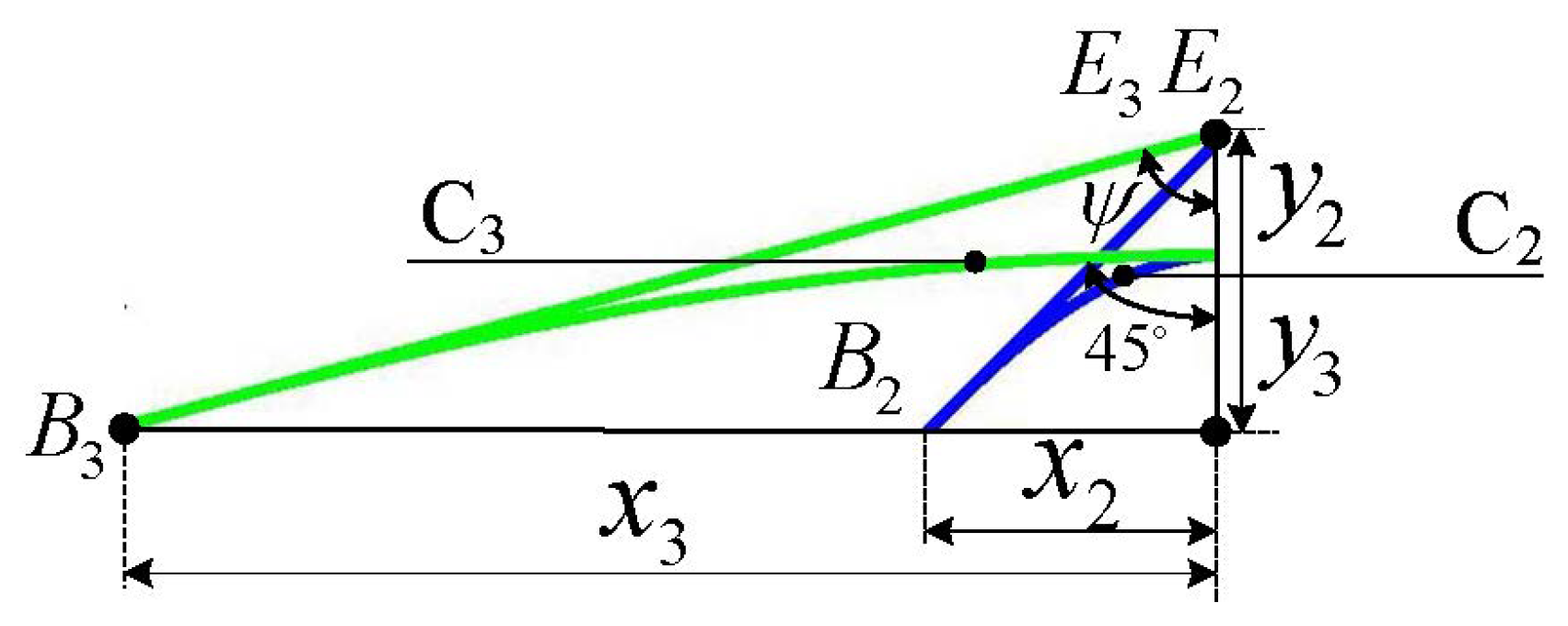
Conform Lamé curve C 2 to curve C 3 in order to make the difference of the orientation angles A 3 E 3 B 3 = 2 ψ . Since y 3 = y 2 and x 3 = x 2 tan ψ , the parametric equation of Lamé curve C 3 can be obtained by using the scaling transformation from that of curve C 2 , i.e., p 3 = S ψ ( tan ψ , 1 ) p 2 , as shown in Figure 8, with p 3 defined as the position vector of an arbitrary point on Lamé curve C 3 . For this curve, two tangent lines stemming from points A 3 and B 3 meet at point E 3 (coinciding with E 2 ), at an angle A 3 E 3 B 3 = C M k T k .
Step 3:
Isotropically scale (An isotropic planar scaling is a resizing of a planar figure by means of identical scalar factors in two orthogonal directions.) Lamé curve C 3 to curve C 4 according to the distance l 2 . Letting the scaling factor be k 1 , and the length of segment B 3 E 3 ¯ be l 0 , k 1 = l 2 / l 0 . Hence, the parametric equation of Lamé curve C 4 can be obtained by using the isotropically scaling transformation from that of curve C 3 , i.e., p 4 = S k ( k 1 , k 1 ) p 3 , with p 4 defined as the position vector of an arbitrary point on Lamé curve C 4 . It is noteworthy that isotropic scaling changes the size of Lamé curve C 3 but preserves its shape, i.e., the length of segment B 4 E 4 ¯ is changed to l 2 , while A 4 E 4 B 4 remains equal to A 3 E 3 B 3 . In this step, Lamé curve C 4 has the size and shape required by the final trajectory.
Step 4:
Displace Lamé curve C 4 to the final trajectory, making points B 4 , E 4 and A 4 coincide with points C, M k and T k , respectively. Store the homogeneous coordinates of points B j , E j , A j , C, M k and T k into arrays b j , e j , a j , c k , m k and t k , respectively. Define five homogeneous coordinate matrices: N j = [ b j e j a j ], for i = 1 , 2 , 3 , 4 , and N 5 = [ c k m k t k ], whose vector blocks are all three dimensional — their entries are the homogeneous coordinates of the corresponding points in the platform frame F . Then, find a homogeneous displacement matrix D satisfying N 5 = D N 4 ; hence, D = N 5 N 4 1 . Finally, the homogeneous coordinates of the trajectory are calculated as the product of these affine transformations starting from Lamé curve C 1 , i.e.,
p 5 = N 5 N 4 1 S k ( k 1 , k 1 ) S ψ ( tan ψ , 1 ) R ( π / 4 ) p 1
with matrix N 4 given by
N 4 = S k ( k 1 , k 1 ) S ψ ( tan ψ , 1 ) R ( π / 4 ) N 1
where matrices N 1 and N 5 are obtained from the homogeneous coordinates of the starting points B 1 , E 1 and A 1 on curve C 1 , and the desired points C, M k and T k on the final trajectory. These matrices are
N 1 = 0 1 1 1 1 0 1 1 1 , N 5 = 0 0 l 2 sin e θ 0 l 2 l 2 ( 1 + cos e θ ) 1 1 1
In order to simplify the calculation, steps 3 and 4 are combined to obtain the homogeneous coordinates of the trajectory from Lamé curve C 3 directly, i.e.,
p 5 = N 5 N 3 1 S ψ ( tan ψ , 1 ) R ( π / 4 ) p 1
with matrix N 3 given by
N 3 = S ψ ( tan ψ , 1 ) R ( π / 4 ) N 1
According to Equations (24)–(26), the composite affine transformation matrix is calculated as
T 5 N 5 N 3 1 S ψ ( tan ψ , 1 ) R ( π / 4 ) = 0 l 3 l 3 l 2 l 4 l 4 0 0 1
with l 3 and l 4 defined as
l 3 = l 2 sin e θ , l 4 = l 2 cos e θ

4.3. Tracking Scheme

Let the curvature of Lamé curve Cj and the trajectory be κ j and κ 5 , respectively. When the DWMR moves along the trajectory at a velocity v c , the robot twist is constrained by
ω = κ 5 v c
Based on Equations (10) and (29), when the DWMR moves along the trajectory, the actuated joint rates follow in terms of κ 5 :
θ ˙ 1 = v c r ( 1 + l κ 5 ) , θ ˙ 2 = v c r ( 1 l κ 5 )
If the DWMR tracks the trajectory at a velocity v c ( t ) , the time-derivatives of the actuated joint rates are
θ ¨ 1 = v ˙ c r ( 1 + l κ 5 ) + v c r l κ ˙ 5 , θ ¨ 2 = v ˙ c r ( 1 l κ 5 ) v c r l κ ˙ 5
As shown in Figure 4, when the actuated joint rates and accelerations are obtained, the desired torques can be readily calculated based on the inverse dynamics model of Equation (14). It is noteworthy that although path tracking is first implemented by means of the Lamé curve blending technique at the level of kinematic control, it is finally converted into the torque control at the dynamic level. Moreover, this multi-loop vision guidance framework is carried out in the receding-horizon mode, implying multi-step planning but one-step control.

5. Simulation Tests

In order to validate the foregoing technique based on curve blending for DWMRs, numerical simulation tests are conducted in the context of geometric trajectory planning, kinematic trajectory tracking and dynamic torque computation. The geometric, kinematic and inertial parameters of the DWMR at hand are given in Table 2 and Table 3. Moreover, the friction coefficient is β = 2 Ns/rad, the rated torque of the onboard motors being τ r = 20 Nm.
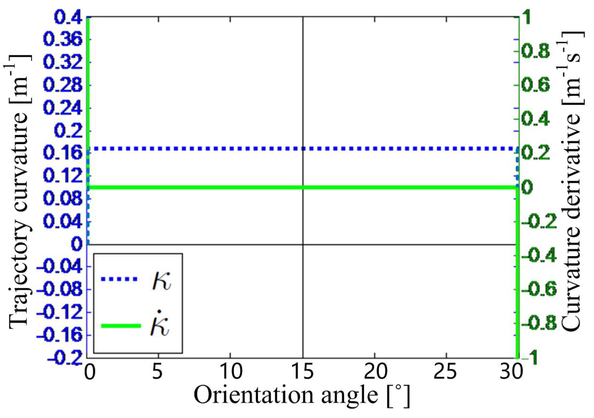
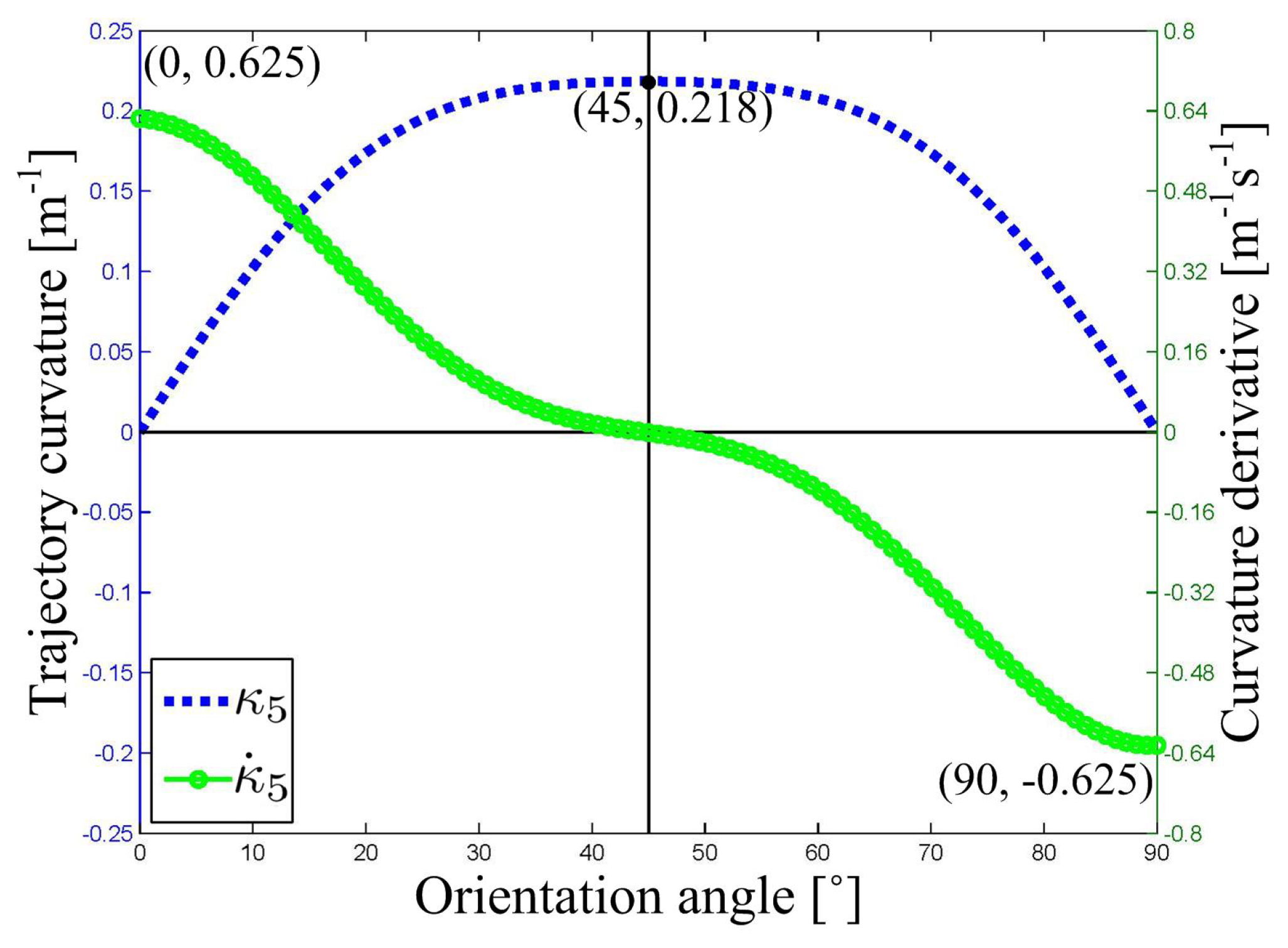
The posture errors are detected as e θ = 30 and l 2 = 1.6 m. The trajectory from the current posture of the DWMR to the guide path is obtained by means of different curves: one is a circular arc, and the other is an affine transformed Lamé curve. The trajectory curvature and its time-derivative are illustrated in Figure 9 and Figure 10, respectively. In Figure 9, the curvature κ of the circular arc has a positive step change from 0 to 0.16 m 1 at the starting point, another negative step change from 0.16 to 0 m 1 at the ending point, and a constant value on the trajectory between these two points. Consequently, one positive and negative impulse occur on the curvature rate of change (RoC) κ ˙ for the circular arc at these two end-points. On the contrary, in Figure 10, the curvature κ 5 of the Lamé curve has a smooth increasing change from 0 m 1 at the starting point, to 0.218 m 1 at the middle point, and then has a smooth decreasing change to 0 m 1 at the ending point. As a result, the curvature RoC κ 5 ˙ of the Lamé curve still remains a smooth curve, changing from an initial finite positive value, going across the 0 value, and reaching a terminal finite negative value.
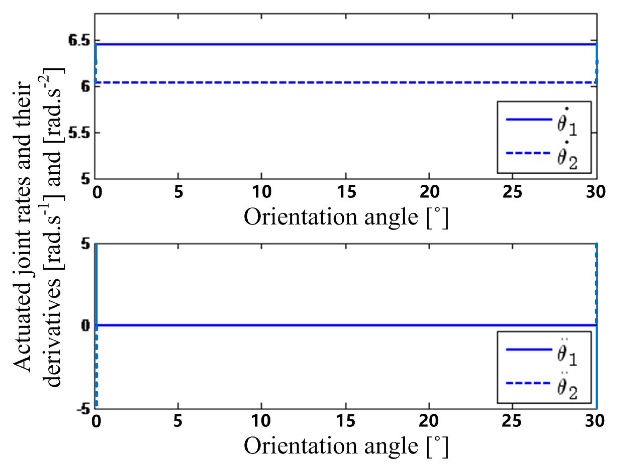
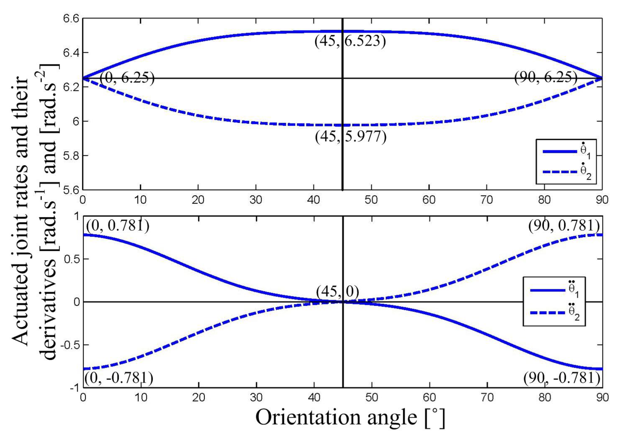
For a constant velocity, v c = 0.5 m/s, the actuated joint rates and their time-derivatives on different trajectories are calculated based on Equations (30) and (31), as shown in Figure 11 and Figure 12, respectively. In Figure 11, the actuated joint rate θ ˙ 1 of the left wheel has a positive step change from 6.25 to 6.5 rad·s 1 at the starting point, another negative step change from 6.5 to 6.25 rad·s 1 at the ending point, and a constant value on the trajectory between these two points. Consequently, one positive and negative impulse occur on the angular acceleration θ ¨ 1 of the left wheel for the circular arc at these two end-points. On the contrary, in Figure 12, the actuated joint rate θ ˙ 1 of the left wheel on the Lamé curve has a smooth increasing change from 6.25 rad·s 1 at the starting point, to 6.523 rad·s 1 at the middle point, and then has a smooth decreasing change to 6.25 rad·s 1 at the ending point. As a result, the angular acceleration θ ¨ 1 of the left wheel for the Lamé curve remains smooth, changing from an initial finite positive value, going across the 0 value, and reaching a terminal finite negative value. From Figure 10 and Figure 12, it is apparent that the trajectory curvature of the Lamé curve and the actuated joint rates of the two wheels on the curve are significantly flat in the middle section.
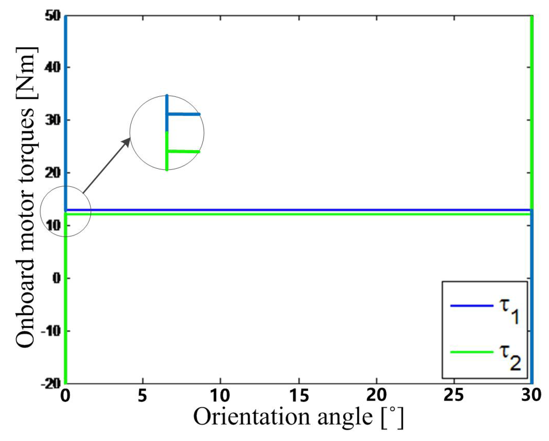
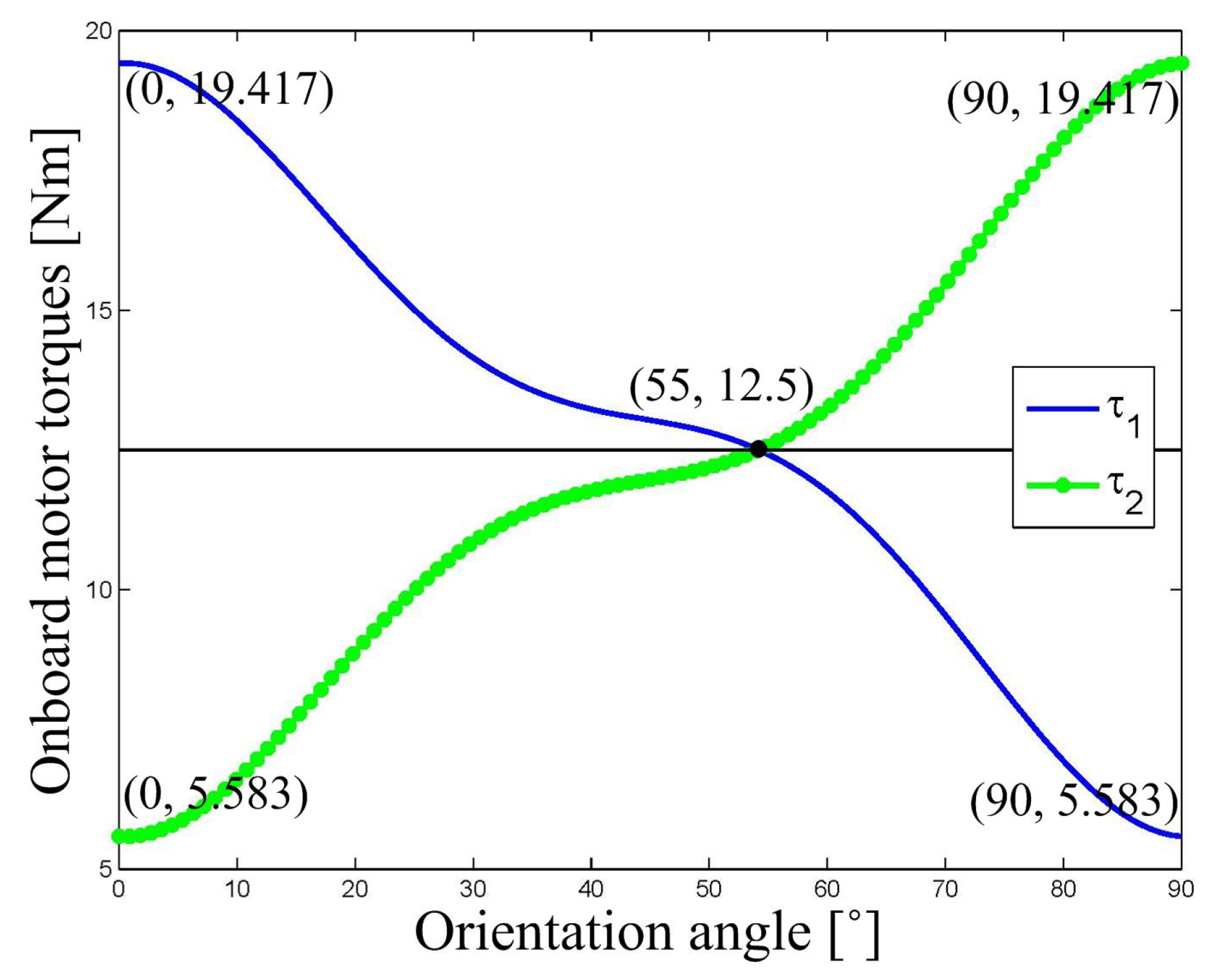
Fianlly, the required torques of the onboard motors of the two driving wheels are computed for the DWMR to move along different trajectories, as shown in Figure 13 and Figure 14, respectively. In Figure 13, the motor torque of the left wheel has a positive impulse at the starting point, another negative impulse at the ending point, and a constant value on the trajectory between these two points. It is noteworthy that the amplitude of the torque impulse is more than 50 Nm, exceeding the rated torque of the onboard motors. On the contrary, in Figure 14, the motor torque of the left wheel for the Lamé curve remains smooth, changing from an initial finite positive value, going across the 0 value, and reaching a terminal finite negative value. The maximum amplitude of the motor torque is always kept below the rated torque.
Moreover, the simulation results reflect the stepwise processing result of the multi-loop vision guidance framework. In the first step, a Lamé-curve trajectory is generated by kinematic path tracking, with its shape as shown in Figure 7, and pertinent parameters, as shown in Figure 10. In the second step, the actuated joint rates and angular accelerations are calculated based on the inverse-kinematics model, as shown in Figure 12. In the third step, the required wheel torques are computed based on the inverse-dynamics model, as shown in Figure 14.

6. Conclusions

Applying computer vision to mobile robot navigation has been studied for more than two decades. Cameras can be fixed on the ceiling with a large field of view, or mounted on the mobile robot with a high recognition accuracy. The limited field of view of onboard cameras brings great difficulties to path tracking of DWMRs in high-speed manoeuvres. In order to cope with the demands of the latter, a multi-loop receding-horizon control framework, including path tracking, robot control, and drive control, is proposed for vision guidance of mobile robots. Lamé curves are used to synthesize a trajectory with G 2 -continuity in the field of view of the mobile robot for path tracking, from its current posture towards the guide path. The whole multi-loop control process, from Lamé-curve blending to computational torque control, is carried out iteratively by means of the receding-horizon strategy. In simulation tests, a circular arc and a Lamé curve are, respectively, used as the blending trajectory for the vision guidance approach. The comparison of trajectory curvature, actuated joint rates and motor torques shows the effectiveness of the vision guidance approach based on Lamé-curve blending. In future research work, our guidance control approach will probably be experimentally integrated with a practical vision guidance system, and further validated on a vision-guided mobile robot running in a shop-floor environment.

Author Contributions

X.W. and J.A. formulated the problems and constructed the research framework; X.W., T.Z. and Q.S. devised the methodologies and designed the experiments; X.W. and C.S. conducted the experiments; C.S. and L.W. provided analysis tools and analyzed the data; X.W. and T.Z. wrote the original draft; J.A., X.W. and T.Z. contributed to the revision, editing and formatting of the paper. All authors have read and agreed to the published version of the manuscript.

Funding

This research work was supported by the National Natural Science Foundation of China (grant number: 61973154), the Natural Sciences and Engineering Research Council of Canada (grant number: 4532-2010), McGill University’s James McGill Professorship of Mechanical Engineering (grant number: 100711), the National Defense Basic Scientific Research Program of China (grant number: JCKY2018605C004), and the Fundamental Research Funds for the Central Universities of China (grant number: NS2019033).

Conflicts of Interest

The authors declare no conflict of interest.

References

  1. Jin, X.B.; Su, T.L.; Kong, J.L.; Bai, Y.T.; Miao, B.B.; Dou, C. State-of-the-art mobile intelligence: Enabling robots to move like humans by estimating mobility with artificial intelligence. Appl. Sci. 2018, 8, 379. [Google Scholar] [CrossRef] [Green Version]
  2. Durrant-Whyte, H. Where am I? A tutorial on mobile vehicle localization. Ind. Robot. 1994, 21, 11–16. [Google Scholar] [CrossRef]
  3. Skulstad, R.; Li, G.; Fossen, T.I.; Vik, B.; Zhang, H. Dead reckoning of dynamically positioned ships: Using an efficient recurrent neural network. IEEE Robot. Autom. Mag. 2019, 26, 39–51. [Google Scholar] [CrossRef] [Green Version]
  4. Vale, A.; Ventura, R.; Lopes, P.; Ribeiro, I. Assessment of navigation technologies for automated guided vehicle in nuclear fusion facilities. Robot. Auton. Syst. 2017, 97, 153–170. [Google Scholar] [CrossRef]
  5. Salichs, M.A.; Moreno, L. Navigation of mobile robots: Open questions. Robotica 2000, 18, 227–234. [Google Scholar] [CrossRef]
  6. Seder, M.; Baotic, M.; Petrovic, I. Receding horizon control for convergent navigation of a differential drive mobile robot. IEEE Trans. Control Syst. Technol. 2017, 25, 653–660. [Google Scholar] [CrossRef]
  7. Coelho, P.; Nunes, U. Path following control of a robotic wheelchair. IFAC Proc. Vol. 2004, 37, 179–184. [Google Scholar] [CrossRef]
  8. Shojaei, K.; Shahri, A.M.; Tarakameh, A.; Tabibian, B. Adaptive trajectory tracking control of a differential drive wheeled mobile robot. Robotica 2011, 29, 391–402. [Google Scholar] [CrossRef]
  9. Zhu, X.; Kim, Y.; Merrell, R.; Minor, M.A. Cooperative motion control and sensing architecture in compliant framed modular mobile robots. IEEE Trans. Robot. 2007, 23, 1095–1101. [Google Scholar]
  10. Bianco, C.G.L. Minimum-jerk velocity planning for mobile robot applications. IEEE Trans. Robot. 2013, 29, 1317–1326. [Google Scholar] [CrossRef]
  11. Do, K.D. Bounded controllers for global path tracking control of unicycle-type mobile robots. Robot. Auton. Syst. 2013, 61, 775–784. [Google Scholar] [CrossRef]
  12. Coulaud, J.B.; Campion, G.; Bastin, G.; De Wan, M. Stability analysis of a vision-based control design for an autonomous mobile robot. IEEE Trans. Robot. 2006, 22, 1062–1069. [Google Scholar] [CrossRef] [Green Version]
  13. Wu, X.; Shen, W.; Lou, P.; Wu, B.; Wang, L.; Tang, D. An automated guided mechatronic tractor for path tracking of heavy-duty robotic vehicles. Mechatronics 2016, 35, 23–31. [Google Scholar] [CrossRef]
  14. Ko, M.H.; Ryuh, B.S.; Kim, K.C.; Suprem, A.; Mahalik, N.P. Autonomous greenhouse mobile robot driving strategies from system integration perspective: Review and application. IEEE/ASME Trans. Mechatron. 2015, 20, 1705–1716. [Google Scholar] [CrossRef]
  15. Xing, W.; Peihuang, L.; Jun, Y.; Xiaoming, Q.; Dunbing, T. Intersection recognition and guide-path selection for a vision-based AGV in a bidirectional flow network. Int. J. Adv. Robot. Syst. 2014, 11, 39. [Google Scholar] [CrossRef] [Green Version]
  16. Yang, J.L.; Su, D.T.; Shiao, Y.S.; Chang, K.Y. Path-tracking controller design and implementation of a vision-based wheeled mobile robot. Proc. Inst. Mech. Eng. Part I J. Syst. Control Eng. 2009, 223, 847–862. [Google Scholar] [CrossRef]
  17. Yi, J.; Wang, H.; Zhang, J.; Song, D.; Jayasuriya, S.; Liu, J. Kinematic modeling and analysis of skid-steered mobile robots with applications to low-cost inertial-measurement-unit-based motion estimation. IEEE Trans. Robot. 2009, 25, 1087–1097. [Google Scholar]
  18. Khalaji, A.K.; Moosavian, S.A.A. Robust adaptive controller for a tractor-trailer mobile robot. IEEE/ASME Trans. Mechatron. 2014, 19, 943–953. [Google Scholar] [CrossRef]
  19. Beccari, G.; Caselli, S.; Zanichelli, F.; Calafiore, A. Vision-based line tracking and navigation in structured environments. In Proceedings of the 1997 IEEE International Symposium on Computational Intelligence in Robotics and Automation CIRA’97, Towards New Computational Principles for Robotics and Automation, Monterey, CA, USA, 10–11 July 1997; pp. 406–411. [Google Scholar]
  20. Lee, J.; Hyun, C.H.; Park, M. A vision-based automated guided vehicle system with marker recognition for indoor use. Sensors 2013, 13, 10052–10073. [Google Scholar] [CrossRef]
  21. Zhang, H.; Hernandez, D.; Su, Z.; Su, B. A low cost vision-based road-following system for mobile robots. Appl. Sci. 2018, 8, 1635. [Google Scholar] [CrossRef] [Green Version]
  22. Martínez-Barberá, H.; Herrero-Pérez, D. Autonomous navigation of an automated guided vehicle in industrial environments. Robot. Comput. Integr. Manuf. 2010, 26, 296–311. [Google Scholar] [CrossRef]
  23. Morales, J.; Martínez, J.L.; Martínez, M.A.; Mandow, A. Pure-pursuit reactive path tracking for nonholonomic mobile robots with a 2D laser scanner. EURASIP J. Adv. Signal Process. 2009, 3, 935237. [Google Scholar] [CrossRef] [Green Version]
  24. Szepe, T.; Assal, S.F.M. Pure pursuit trajectory tracking approach: Comparison and experimental validation. Int. J. Robot. Autom. 2012, 27, 355–363. [Google Scholar] [CrossRef]
  25. Elbanhawi, M.; Simic, M.; Jazar, R. Receding horizon lateral vehicle control for pure pursuit path tracking. J. Vib. Control 2018, 24, 619–642. [Google Scholar] [CrossRef]
  26. Wu, X.; Angeles, J.; Zou, T.; Xiao, H.; Li, W.; Lou, P. Steering-angle computation for the multibody modelling of differential-driving mobile robots with a caster. Int. J. Adv. Robot. Syst. 2018, 12, 1–13. [Google Scholar] [CrossRef] [Green Version]
  27. Kim, Y.; Kim, B.K. Efficient time-optimal two-corner trajectory planning algorithm for differential-driven wheeled mobile robots with bounded motor control inputs. Robot. Auton. Syst. 2015, 64, 35–43. [Google Scholar] [CrossRef]
  28. Hwang, C. Comparison of path tracking control of a car-like mobile robot with and without motor dynamics. IEEE/ASME Trans. Mechatron. 2016, 21, 1801–1811. [Google Scholar] [CrossRef]
  29. Zhou, D.; Zhang, Y.Q.; Li, S.L. Receding horizon guidance and control using sequential convex programming for spacecraft 6-DOF close proximity. Aerosp. Sci. Technol. 2019, 87, 459–477. [Google Scholar] [CrossRef]
  30. Chen, D.; Lu, Q.; Peng, D.; Yin, K.; Zhong, C.; Shi, T. Receding horizon control of mobile robots for locating unknown wireless sensor networks. Assembly Autom. 2019, 39, 445–459. [Google Scholar] [CrossRef]
  31. Dauod, H.; Serhan, D.; Wang, H.; Khader, N.; Yoon, S.W.; Srihari, K. Robust receding horizon control strategy for replenishment planning of pharmacy robotic dispensing systems. Robot Comput. Integr. Manuf. 2019, 59, 177–188. [Google Scholar] [CrossRef]
  32. Wu, X.; Sun, C.; Zou, T.; Xiao, H.; Wang, L.; Zhai, J. Intelligent path recognition against image noises for vision guidance of automated guided vehicles in a complex workspace. Appl. Sci. 2019, 9, 4108. [Google Scholar] [CrossRef] [Green Version]
  33. Angeles, J. The role of the rotation matrix in the teaching of planar kinematics. Mech. Mach. Theory 2015, 89, 28–37. [Google Scholar] [CrossRef]
  34. Angeles, J. The natural orthogonal complement. In Fundamentals of Robotic Mechanical Systems: Theory, Methods, Algorithms, 4th ed.; Springer: New York, NY, USA, 2014; pp. 306–316. [Google Scholar]
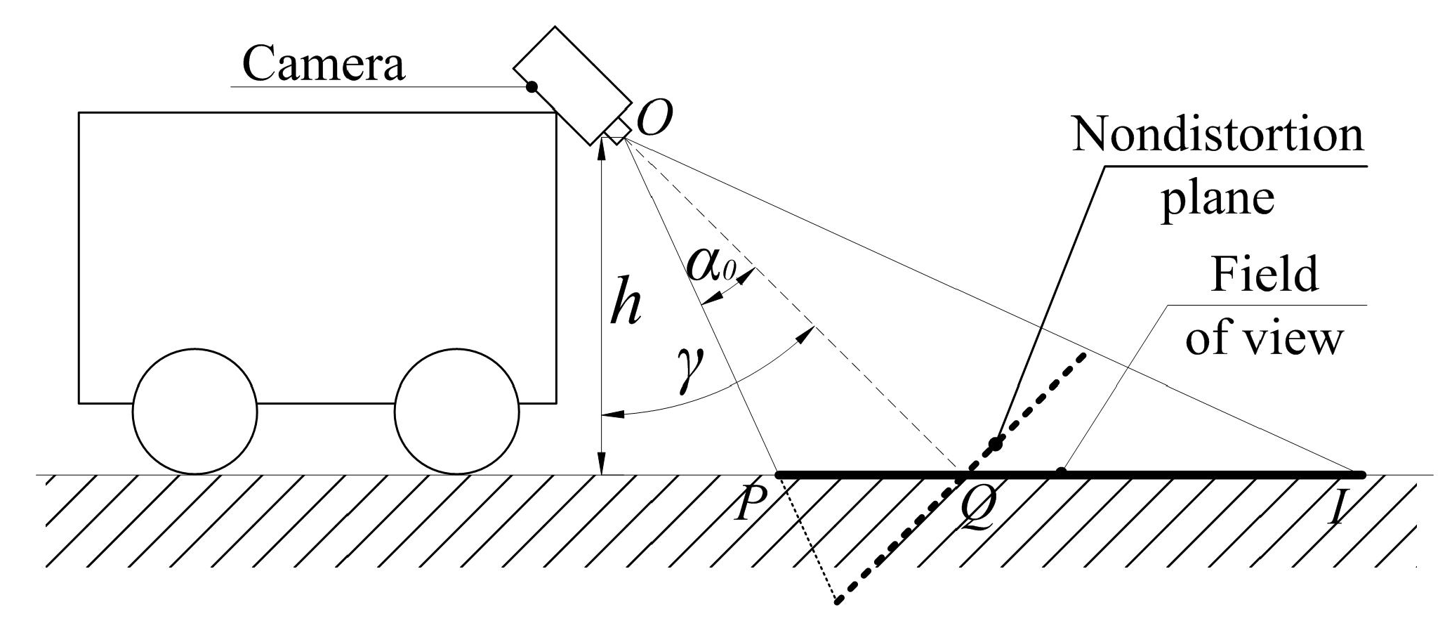
Figure 1. The field of view of an onboard camera.
Applsci 10 00676 g001
Figure 2. Top view of path tracking of a DWMR.
Applsci 10 00676 g002
Figure 3. Path approaching within the field of view.
Applsci 10 00676 g003
Figure 4. A closed-loop receding-horizon control framework.
Applsci 10 00676 g004
Figure 5. Diagram of a DWMR.
Applsci 10 00676 g005
Figure 6. Path tracking based on trajectory blending.
Applsci 10 00676 g006
Figure 7. Affine transformations of Lamé curves for tracking.
Applsci 10 00676 g007
Figure 8. Zoom-in of Lamé curves C 2 and C 3 .
Applsci 10 00676 g008
Figure 9. The curvature of the circular arc and its time-derivative.
Applsci 10 00676 g009
Figure 10. The curvature of the Lamé curve and its time-derivative.
Applsci 10 00676 g010
Figure 11. Actuated joint rates and angular accelerations on the circular arc.
Applsci 10 00676 g011
Figure 12. Actuated joint rates and angular accelerations on the Lamé curve.
Applsci 10 00676 g012
Figure 13. Required motor torques of the DWMR on the circular arc.
Applsci 10 00676 g013
Figure 14. Required motor torques of the DWMR on the Lamé curve.
Applsci 10 00676 g014
Table 1. Linearization error.
Curvature [m]21.81.61.41.21.0
Error [ 10 3 m]5.065.636.347.258.4810.20
Relative error [%]0.2530.3130.3960.5180.7071.02
Table 2. Geometric and kinematic parameters.
r [m]l [m]a [m]b [m] v c [m/s]
0.080.20.180.420.5
Table 3. Inertial parameters.
m 1 2 kg I x 0.0064 kg·m 2 I y 0.0032 kg·m 2
m 2 2 kg I z 0.0032 kg·m 2 I 3 104 kg·m 2
m 3 200 kg H 4 0.0192 kg·m 2 H 5 8.8581 kg·m 2