Deep Learning for Black-Box Modeling of Audio Effects †


Abstract
1. Introduction
2. Background
2.1. Modeling of Nonlinear Audio Effects
2.2. Modeling of Time-Varying Audio Effects
2.3. Deep Learning for Audio Effects Modeling
3. Methods
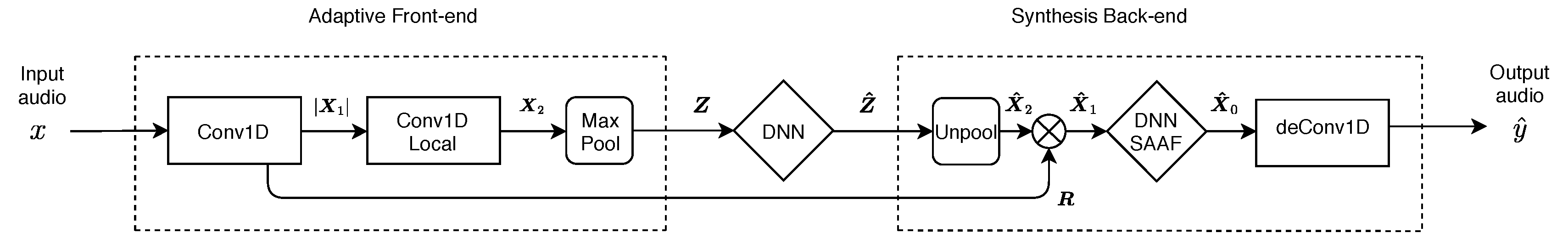
3.1. Convolutional Audio Effects Modeling Network: CAFx
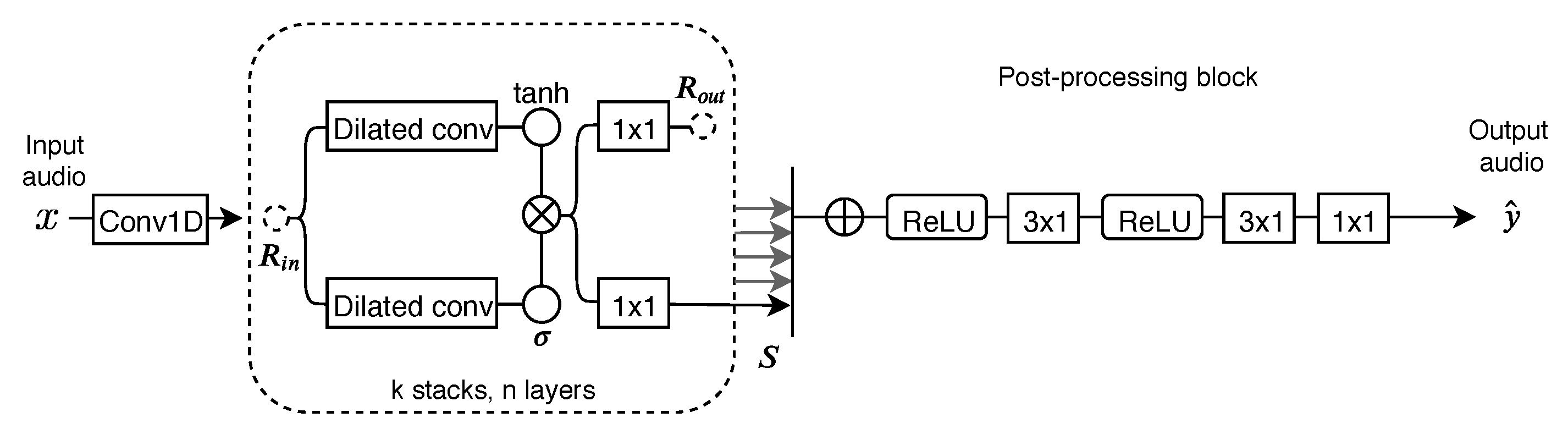
3.2. Feedforward WaveNet Audio Effects Modeling Network—WaveNet
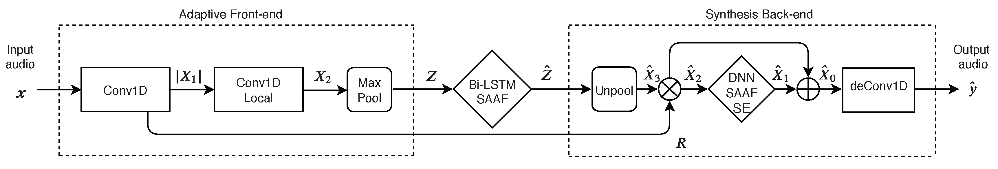
3.3. Convolutional Recurrent Audio Effects Modeling Network—CRAFx
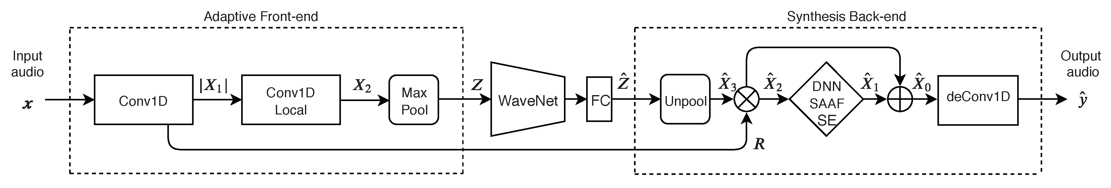
3.4. Convolutional and WaveNet Audio Effects Modeling Network - CWAFx
4. Experiments
4.1. Training
4.2. Dataset
4.2.1. Universal Audio Vacuum-Tube Preamplifier 610-B
4.2.2. Universal Audio Transistor-Based Limiter Amplifier 1176LN
4.2.3. 145 Leslie Speaker Cabinet
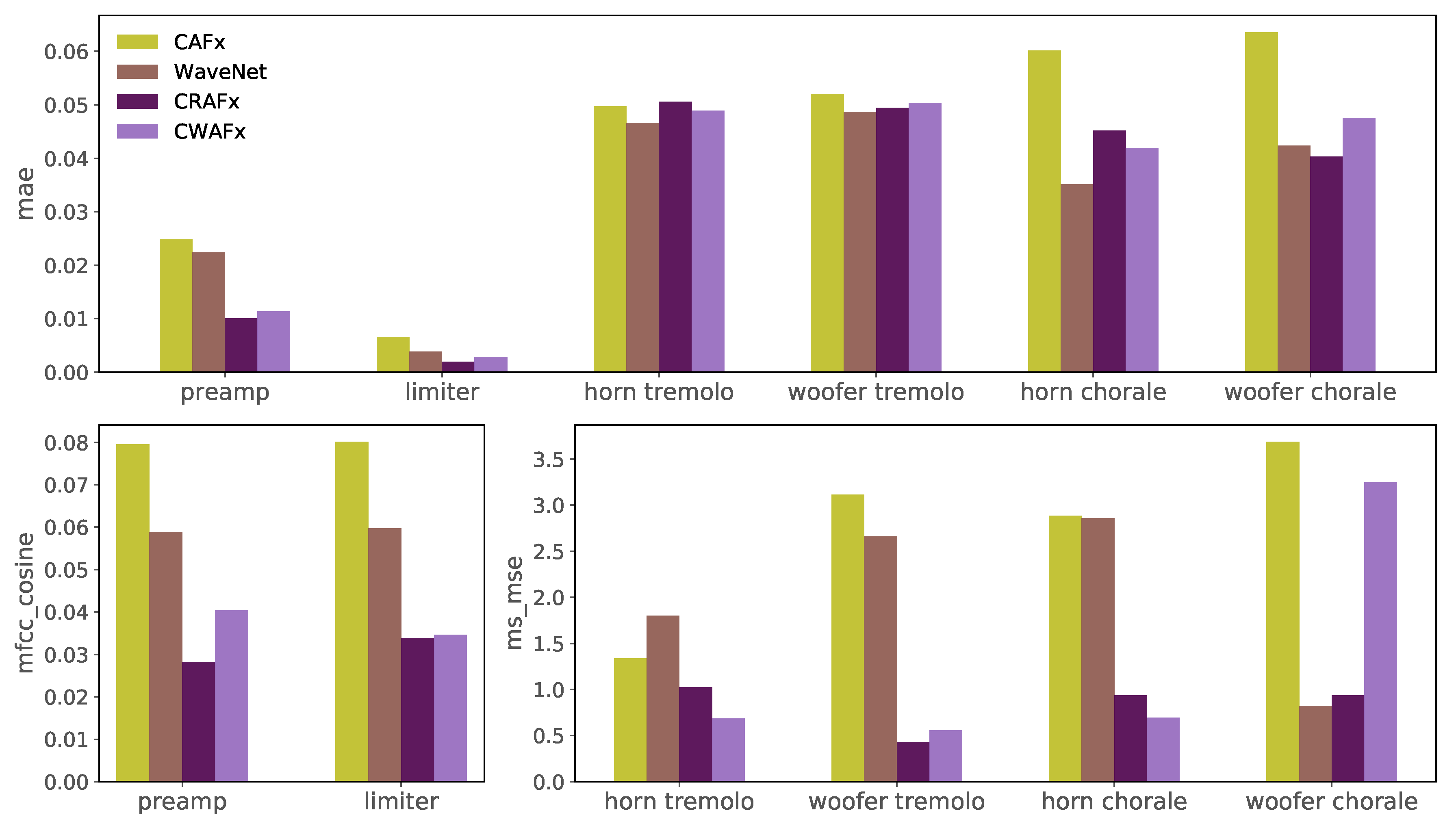
4.3. Objective Metrics
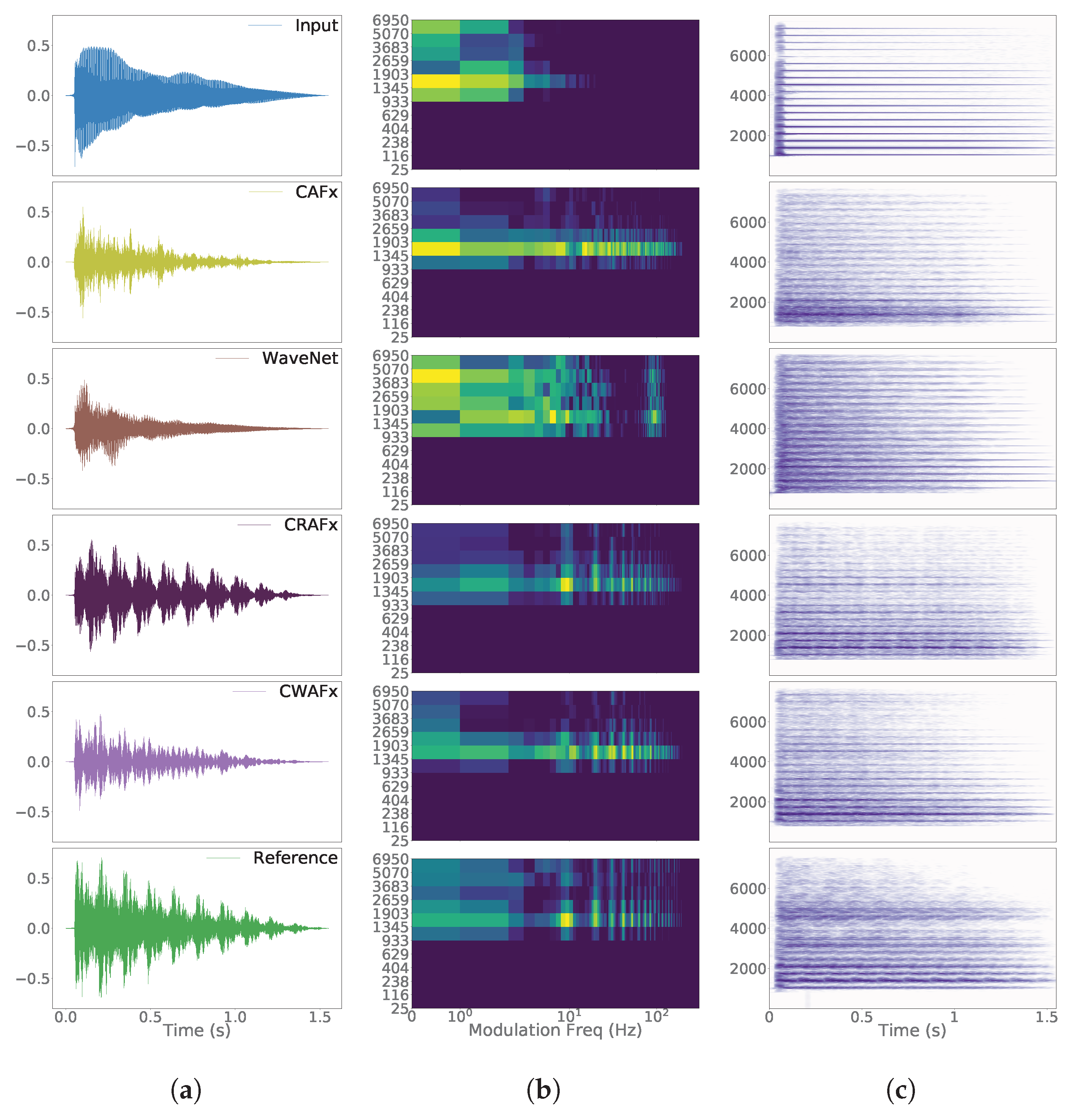
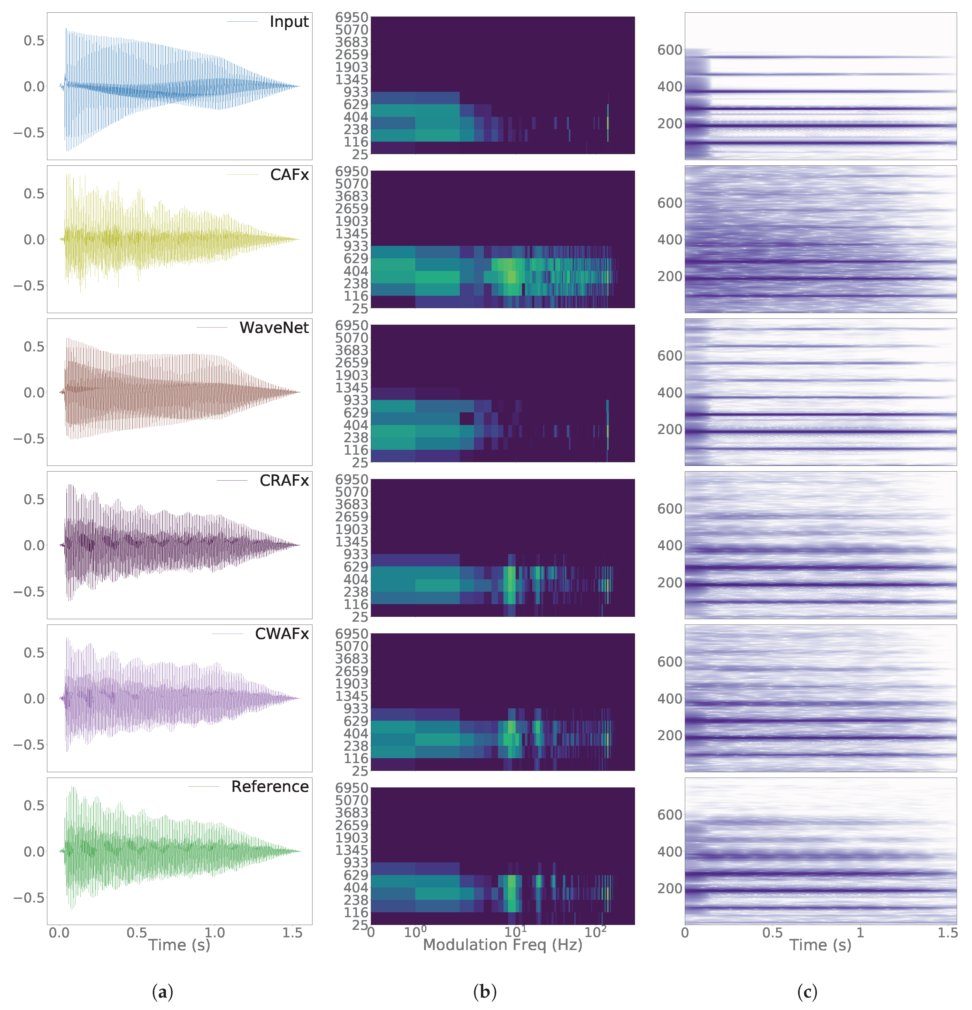
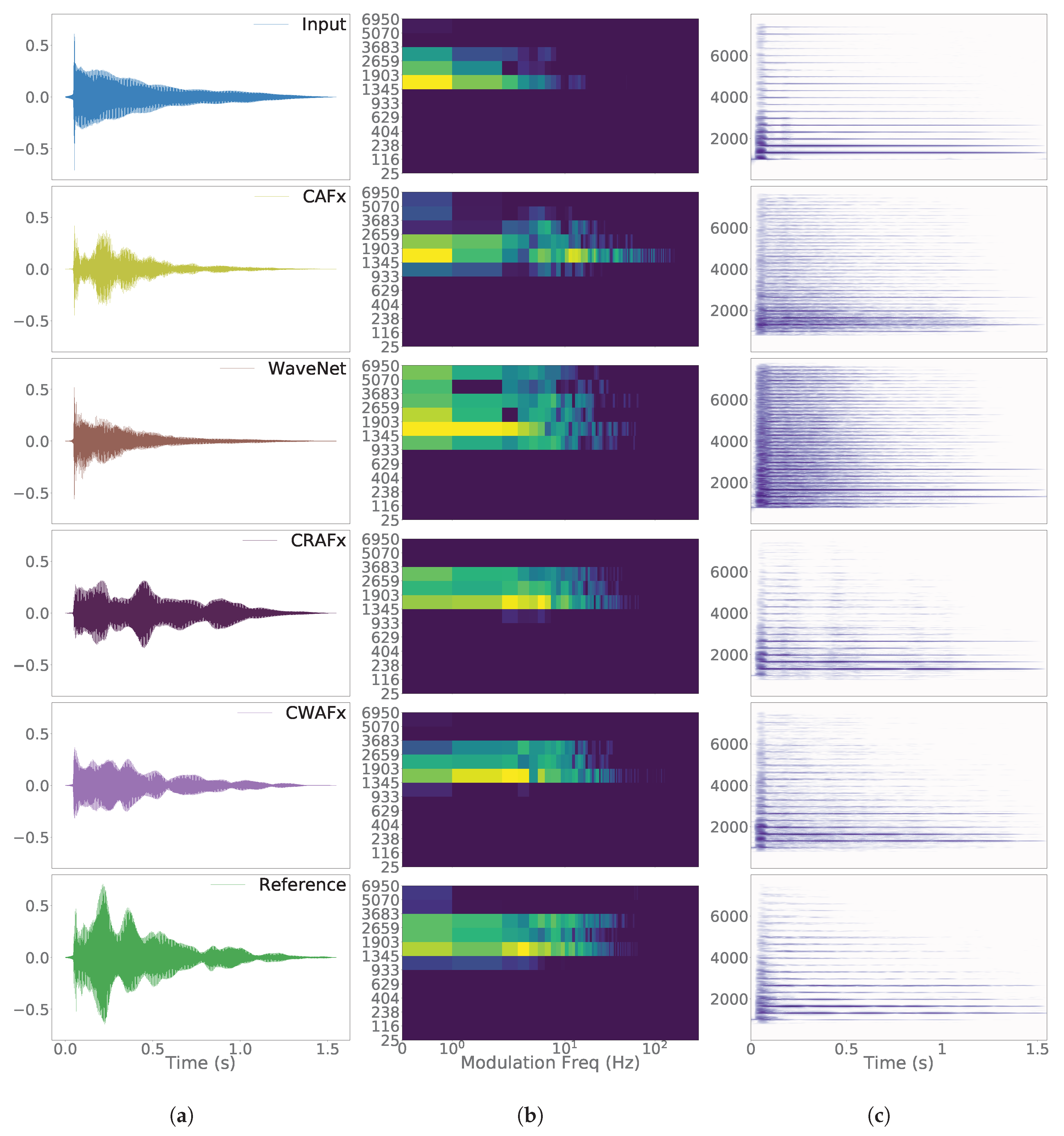
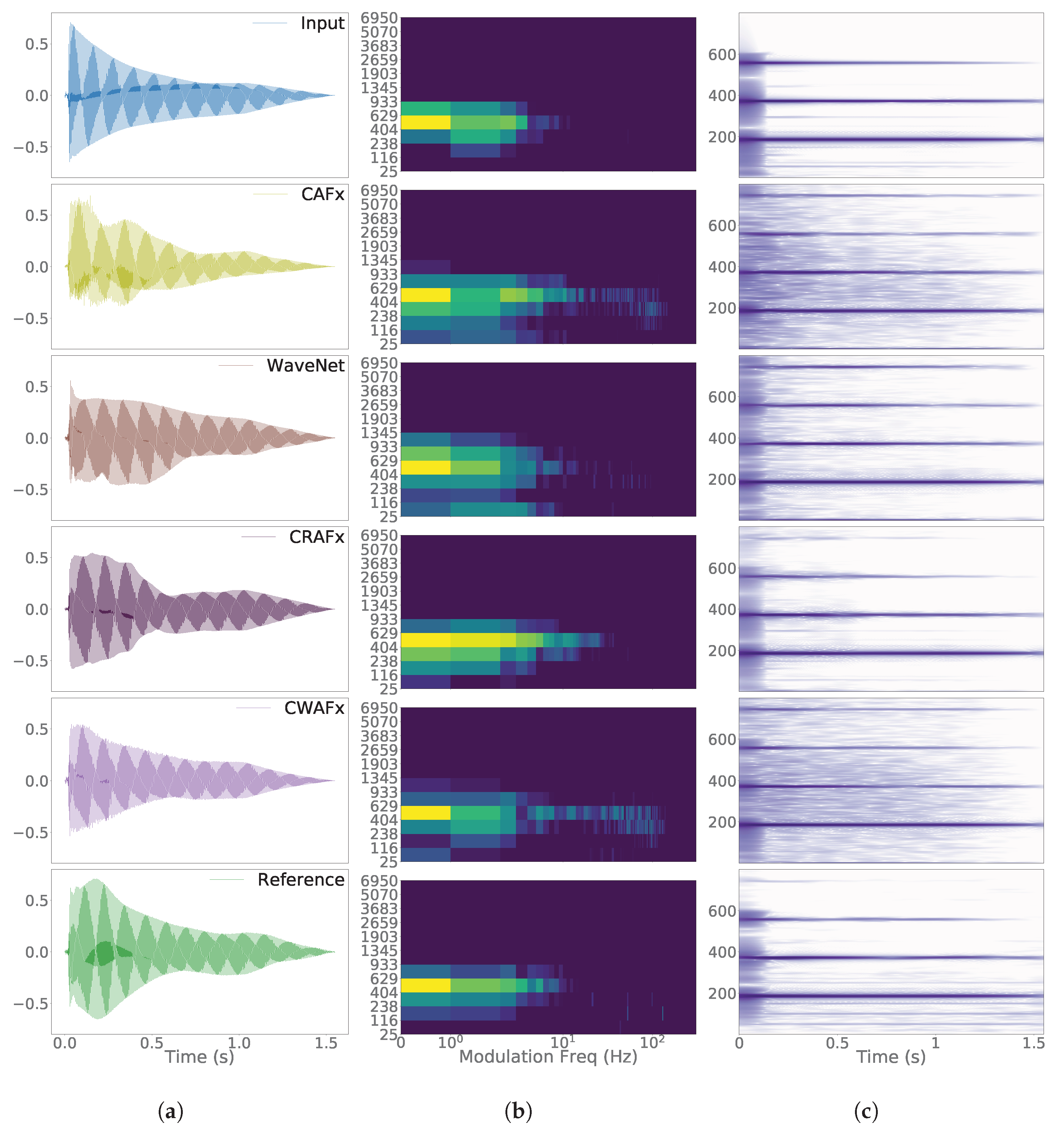
- A Gammatone filter bank is applied to the target and output entire waveforms. In total we use 12 filters, with center frequencies spaced logarithmically from 26 Hz to 6950 Hz.
- The envelope of each filter output is calculated via the magnitude of the Hilbert transform and downsampled to 400 Hz.
- A Modulation filter bank is applied to each envelope. In total we use 12 filters, with center frequencies spaced logarithmically from Hz to 100 Hz.
- The Fast Fourier Transform (FFT) is calculated for each modulation filter output of each Gammatone filter. The energy is summed across the Gammatone and Modulation filter banks and the ms_mse metric is the mean squared error of the logarithmic values of the FFT frequency bins.
- A log-power-melspectogram is computed from the energy-normalized waveforms. This is calculated with 40 mel-bands and audio frames of 4096 samples and hop size.
- 13 MFCCs are computed using the discrete cosine transform and the mfcc_cosine metric is the mean cosine distance across the MFCC vectors.
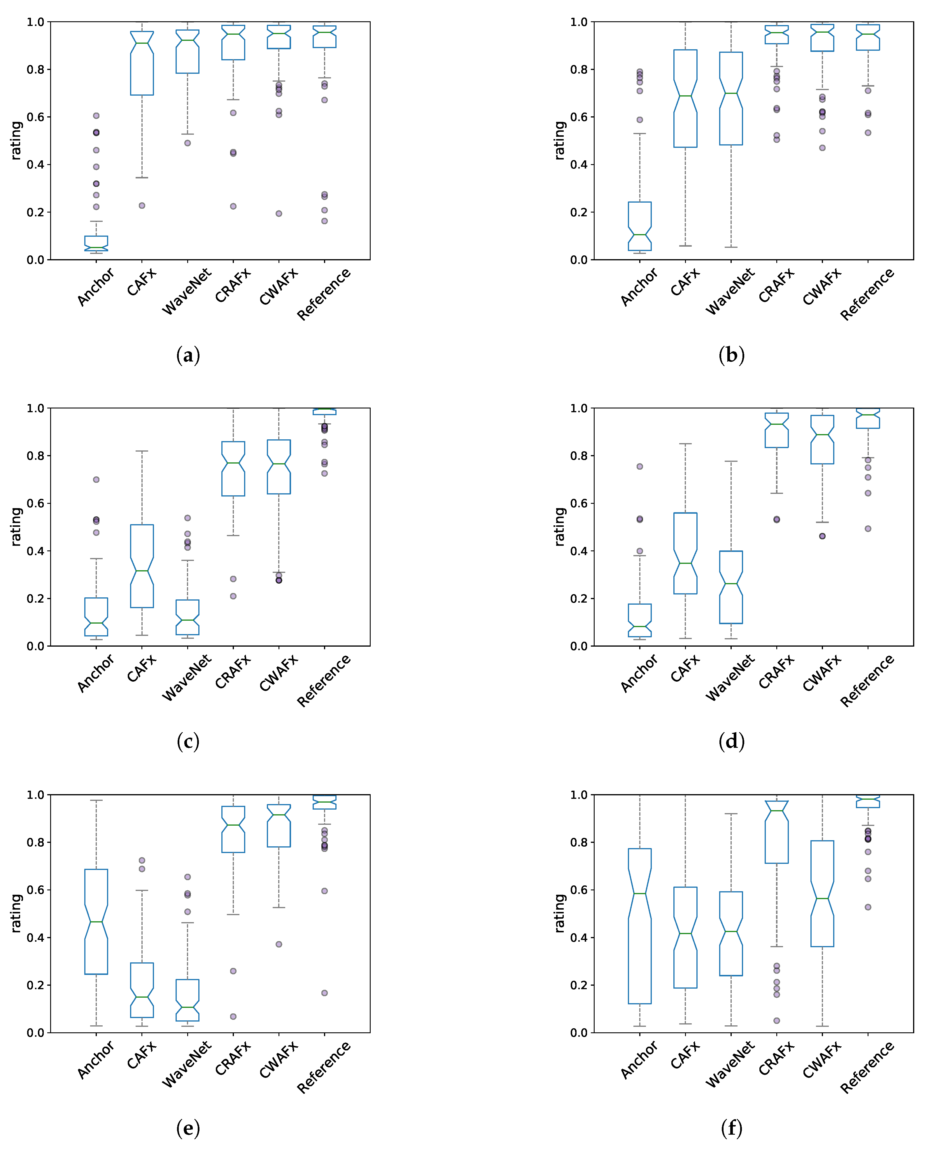
4.4. Listening Test
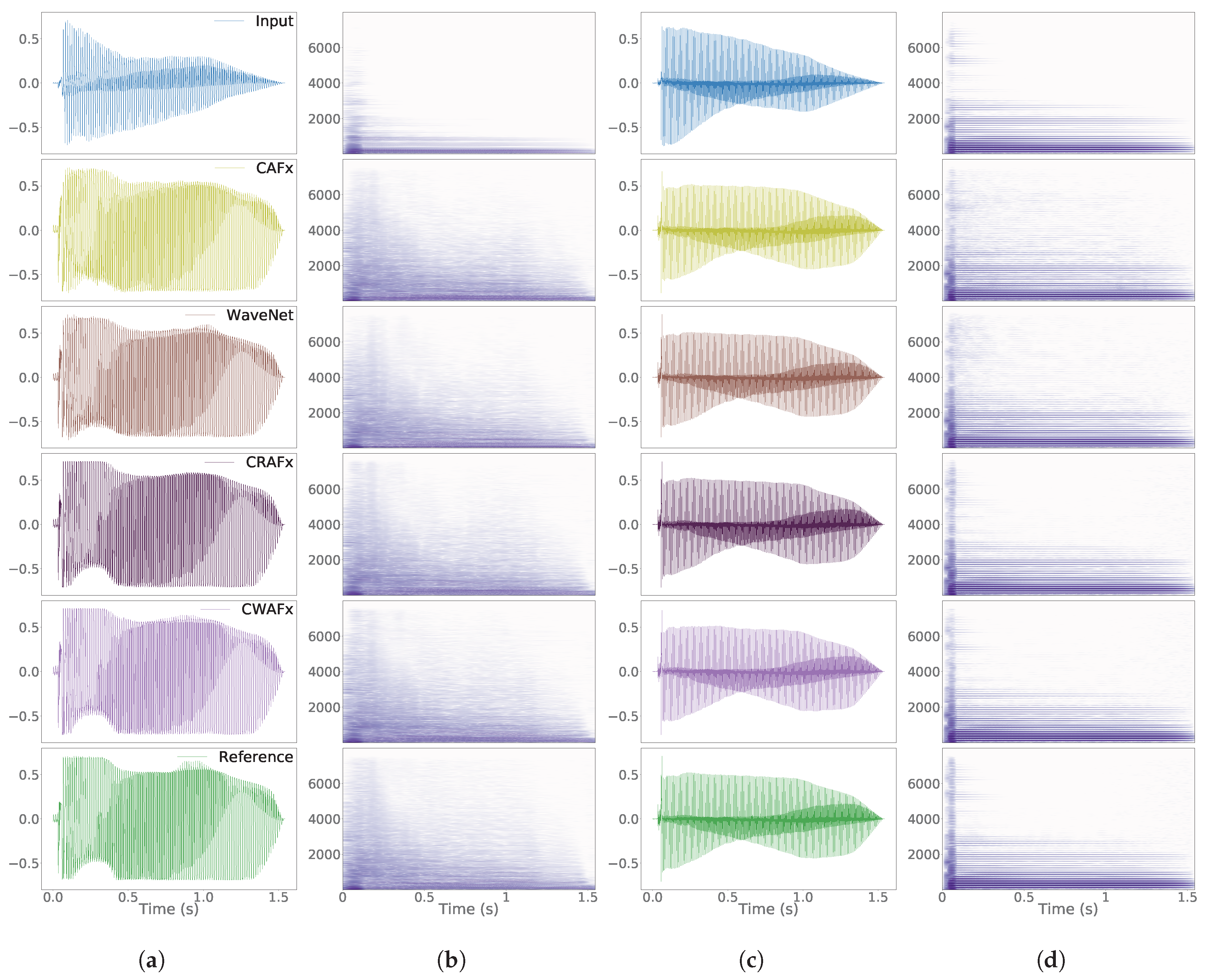
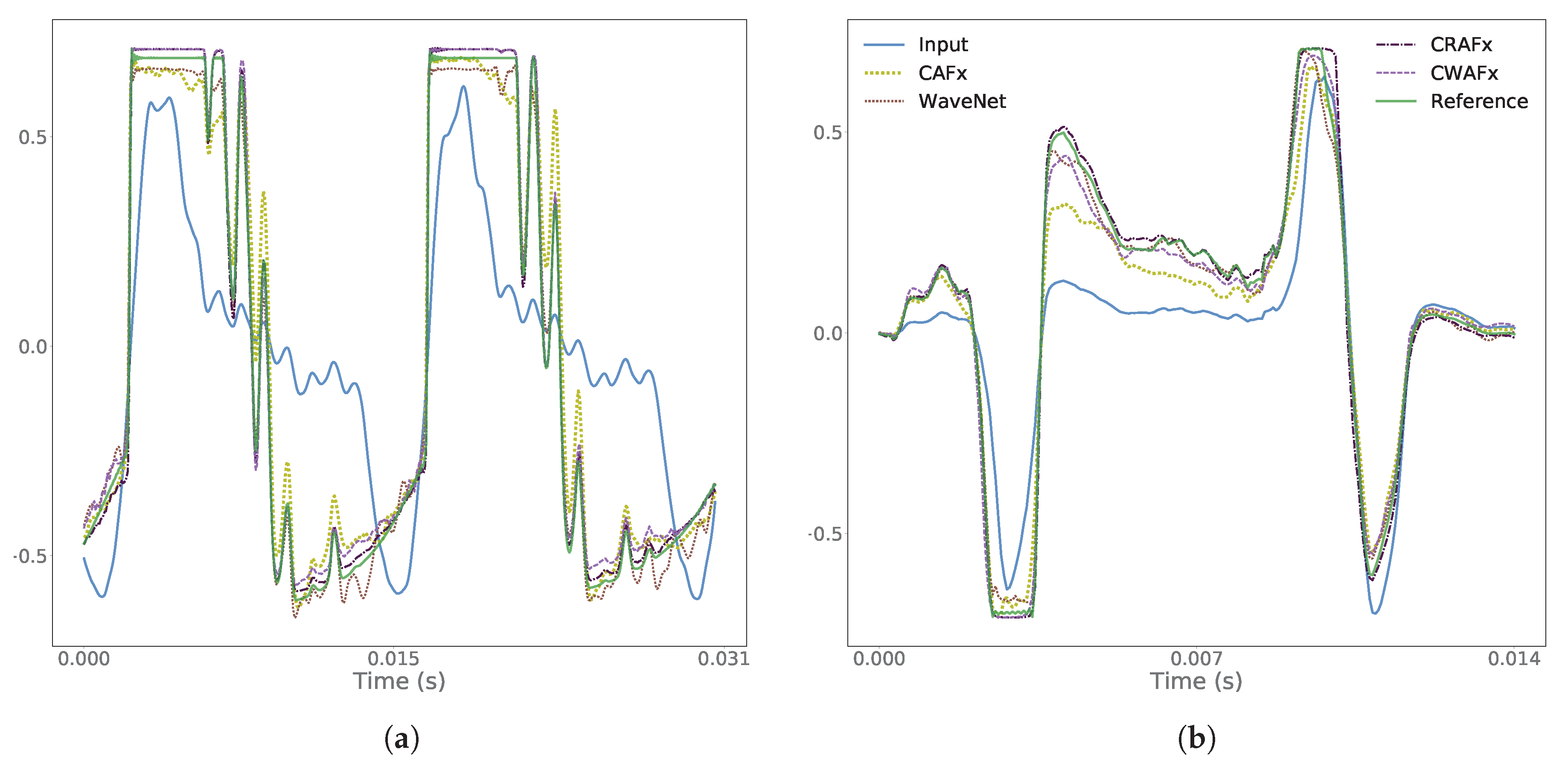
5. Results
6. Discussion
6.1. Nonlinear Task with Short-Term Memory - Preamp
6.2. Time-Dependent Nonlinear Task - Limiter
6.3. Time-Varying Task: Leslie Speaker
7. Conclusions
Author Contributions
Funding
Acknowledgments
Conflicts of Interest
Appendix A

| Model | Number of Parameters | GPU Time (s) | CPU Time (s) |
|---|---|---|---|
| CAFx | 604,545 | 0.0842 | 1.2939 |
| WaveNet | 1,707,585 | 0.0508 | 1.0233 |
| CRAFx | 275,073 | 0.4066 | 2.8706 |
| CWAFx | 205,057 | 0.0724 | 2.9552 |
References
- Smith, J.O. Physical Audio Signal Processing: For Virtual Musical Instruments and Audio Effects; W3K Publishing. 2010. Available online: http://www.w3k.org/books/ (accessed on 10 November 2019).
- Zölzer, U. DAFX: Digital Audio Effects; John Wiley & Sons: Hoboken, NJ, USA, 2011. [Google Scholar]
- Puckette, M. The Theory and Technique of Electronic Music; World Scientific Publishing Company: Singapore, 2007. [Google Scholar]
- Reiss, J.D.; McPherson, A. Audio Effects: Theory, Implementation and Application; CRC Press: Boca Raton, FL, USA, 2014. [Google Scholar]
- Henricksen, C.A. Unearthing the mysteries of the leslie cabinet. Recording Engineer/Producer Magazine, April 1981. [Google Scholar]
- Martínez Ramírez, M.A.; Reiss, J.D. End-to-end equalization with convolutional neural networks. In Proceedings of the 21st International Conference on Digital Audio Effects (DAFx-18), Aveiro, Portugal, 4–8 September 2018. [Google Scholar]
- Martínez Ramírez, M.A.; Reiss, J.D. Modeling of nonlinear audio effects with end-to-end deep neural networks. In Proceedings of the IEEE International Conference on Acoustics, Speech, and Signal Processing (ICASSP), Brighton, UK, 12–17 May 2019. [Google Scholar]
- Martínez Ramírez, M.A.; Benetos, E.; Reiss, J.D. A general-purpose deep learning approach to model time-varying audio effects. In Proceedings of the 22nd International Conference on Digital Audio Effects (DAFx-19), Birmingham, UK, 2–6 September 2019. [Google Scholar]
- Damskägg, E.P.; Juvela, L.; Thuillier, E.; Vesa, V. Deep learning for tube amplifier emulation. In Proceedings of the IEEE International Conference on Acoustics, Speech, and Signal Processing (ICASSP), Brighton, UK, 12–17 May 2019. [Google Scholar]
- Oord, A.v.d.; Dieleman, S. Wavenet: A Generative Model for Raw Audio; Deepmind: London, UK, 2016. [Google Scholar]
- Möller, S.; Gromowski, M.; Zölzer, U. A measurement technique for highly nonlinear transfer functions. In Proceedings of the 5th International Conference on Digital Audio Effects (DAFx-02), Hamburg, Germany, 26–28 September 2002. [Google Scholar]
- Karjalainen, M.; Mäki-Patola, T.; Kanerva, A.; Huovilainen, A. Virtual air guitar. J. Audio Eng. Soc. 2006, 54, 964–980. [Google Scholar]
- Yeh, D.T.; Jonathan, S.A.; Andrei, V.; Smith, J. Numerical methods for simulation of guitar distortion circuits. Comput. Music J. 2008, 32, 23–42. [Google Scholar] [CrossRef]
- Yeh, D.T.; Smith, J.O. Simulating guitar distortion circuits using wave digital and nonlinear state-space formulations. In Proceedings of the 11th International Conference on Digital Audio Effects (DAFx-08), Espoo, Finland, 1–4 September 2008. [Google Scholar]
- Yeh, D.T.; Abel, J.S.; Smith, J.O. Automated physical modeling of nonlinear audio circuits for real-time audio effects Part I: Theoretical development. IEEE Trans. Audio Speech Lang. Proc. 2010, 18, 728–737. [Google Scholar] [CrossRef]
- Abel, J.S.; Berners, D.P. A technique for nonlinear system measurement. In Proceedings of the 121st Audio Engineering Society Convention, San Francisco, CA, USA, 5–8 October 2006. [Google Scholar]
- Hélie, T. On the use of Volterra series for real-time simulations of weakly nonlinear analog audio devices: Application to the Moog ladder filter. In Proceedings of the 9th International Conference on Digital Audio Effects (DAFx-06), Montreal, QC, Canada, 18–20 September 2006. [Google Scholar]
- Gilabert Pinal, P.L.; Montoro López, G.; Bertran Albertí, E. On the Wiener and Hammerstein models for power amplifier predistortion. In Proceedings of the IEEE Asia-Pacific Microwave Conference, Suzhou, China, 4–7 December 2005. [Google Scholar]
- Eichas, F.; Zölzer, U. Black-box modeling of distortion circuits with block-oriented models. In Proceedings of the 19th International Conference on Digital Audio Effects (DAFx-16), Brno, Czech Republic, 5–9 September 2016. [Google Scholar]
- Eichas, F.; Zölzer, U. Virtual analog modeling of guitar amplifiers with Wiener-Hammerstein models. In Proceedings of the 44th Annual Convention on Acoustics (DAGA 2018), Munich, Germany, 19–22 March 2018. [Google Scholar]
- Schmitz, T.; Embrechts, J.J. Nonlinear real-time emulation of a tube amplifier with a Long Short Time Memory neural-network. In Proceedings of the 144th Audio Engineering Society Convention, Milan, Italy, 24–26 May 2018. [Google Scholar]
- Zhang, Z.; Olbrych, E.; Bruchalski, J.; McCormick, T.J.; Livingston, D.L. A vacuum-tube guitar amplifier model using Long/Short-Term Memory networks. In Proceedings of the IEEE SoutheastCon, Tampa Bay Area, FL, USA, 19–22 April 2018. [Google Scholar]
- Wright, A.; Edward, O.; Joseph, B.; Thomas, J.M.; David, L.L. Real-time black-box modelling with recurrent neural networks. In Proceedings of the 22nd International Conference on Digital Audio Effects (DAFx-19), Birmingham, UK, 2–6 September 2019. [Google Scholar]
- Parker, J.; Esqueda, F. Modelling of nonlinear state-space systems using a deep neural network. In Proceedings of the 22nd International Conference on Digital Audio Effects (DAFx-19), Birmingham, UK, 2–6 September 2019. [Google Scholar]
- Kröning, O.; Dempwolf, K.; Zölzer, U. Analysis and simulation of an analog guitar compressor. In Proceedings of the 14th International Conference on Digital Audio Effects (DAFx-11), Paris, France, 19–23 September 2011. [Google Scholar]
- Eichas, F.; Gerat, E.; Zölzer, U. Virtual analog modeling of dynamic range compression systems. In Proceedings of the 142nd Audio Engineering Society Convention, Berlin, Germany, 20–23 May 2017. [Google Scholar]
- Gerat, E.; Eichas, F.; Zölzer, U. Virtual analog modeling of a UREI 1176LN dynamic range control system. In Proceedings of the 143rd Audio Engineering Society Convention, New York, NY, USA, 18–21 October 2017. [Google Scholar]
- Hawley, S.H.; Colburn, B.; Mimilakis, S.I. SignalTrain: Profiling audio compressors with deep neural networks. In Proceedings of the 147th Audio Engineering Society Convention, New York, NY, USA, 21–24 October 2019. [Google Scholar]
- Parker, J. A simple digital model of the diode-based ring-modulator. In Proceedings of the 14th International Conference on Digital Audio Effects (DAFx-11), Paris, France, 19–23 September 2011. [Google Scholar]
- Huovilainen, A. Enhanced digital models for analog modulation effects. In Proceedings of the 8th International Conference on Digital Audio Effects (DAFx-05), Madrid, Spain, 20–22 September 2005. [Google Scholar]
- Eichas, F.; Martin, H.; Udo, Z. Physical modeling of the MXR Phase 90 guitar effect pedal. In Proceedings of the 17th International Conference on Digital Audio Effects (DAFx-14), Erlangen, Germany, 1–5 September 2014. [Google Scholar]
- Bogason, Ó.; Werner, K.J. Modeling circuits with operational transconductance amplifiers using wave digital filters. In Proceedings of the 20th International Conference on Digital Audio Effects (DAFx-17), Edinburgh, Scotland, 5–9 September 2017. [Google Scholar]
- Mačák, J. Simulation of analog flanger effect using BBD circuit. In Proceedings of the 19th International Conference on Digital Audio Effects (DAFx-16), Brno, Czech Republic, 5–9 September 2016. [Google Scholar]
- Smith, J.; Stefania, S.; Jonathan, A.; David, B. Doppler simulation and the Leslie. In Proceedings of the 5th International Conference on Digital Audio Effects (DAFx-02), Hamburg, Germany, 26–28 September 2002. [Google Scholar]
- Pekonen, J.; Pihlajamäki, T.; Välimäki, V. Computationally efficient Hammond organ synthesis. In Proceedings of the 14th International Conference on Digital Audio Effects (DAFx-11), Paris, France, 19–23 September 2011. [Google Scholar]
- Herrera, J.; Hanson, C.; Abel, J.S. Discrete time emulation of the Leslie speaker. In Proceedings of the 127th Audio Engineering Society Convention, New York, NY, USA, 9–12 October 2009. [Google Scholar]
- Holters, M.; Parker, J.D. A combined model for a bucket brigade device and its input and output filters. In Proceedings of the 21st International Conference on Digital Audio Effects (DAFx-17), Aveiro, Portugal, 4–8 September 2018. [Google Scholar]
- Kiiski, R.; Esqueda, F.; Välimäki, V. Time-variant gray-box modeling of a phaser pedal. In Proceedings of the 19th International Conference on Digital Audio Effects (DAFx-16), Brno, Czech Republic, 5–9 September 2016. [Google Scholar]
- Pakarinen, J.; Yeh, D.T. A review of digital techniques for modeling vacuum-tube guitar amplifiers. Comput. Music J. 2009, 33, 85–100. [Google Scholar] [CrossRef]
- Raffel, C.; Smith, J. Practical modeling of bucket-brigade device circuits. In Proceedings of the 13th International Conference on Digital Audio Effects (DAFx-10), Graz, Austria, 6–10 September 2010. [Google Scholar]
- Yeh, D.T. Automated physical modeling of nonlinear audio circuits for real-time audio effects Part II: BJT and vacuum tube examples. IEEE Trans. Audio Speech Lang. Proc. 2012, 20, 1207–1216. [Google Scholar] [CrossRef]
- De Sanctis, G.; Sarti, A. Virtual analog modeling in the wave-digital domain. IEEE Transactions on Audio Speech Lang. Proc. 2009, 18, 715–727. [Google Scholar] [CrossRef]
- Rämö, J.; Välimäki, V. Neural third-octave graphic equalizer. In Proceedings of the 22nd International Conference on Digital Audio Effects (DAFx-19), Birmingham, UK, 2–6 September 2019. [Google Scholar]
- Sheng, D.; Fazekas, G. A feature learning siamese model for intelligent control of the dynamic range compressor. In Proceedings of the International Joint Conference on Neural Networks (IJCNN), Budapest, Hungary, 14–19 July 2019. [Google Scholar]
- Dieleman, S.; Schrauwen, B. End-to-end learning for music audio. In Proceedings of the International Conference on Acoustics, Speech and Signal Processing (ICASSP), Florence, Italy, 4–9 May 2014. [Google Scholar]
- Rethage, D.; Pons, J.; Serra, X. A wavenet for speech denoising. In Proceedings of the IEEE International Conference on Acoustics, Speech and Signal Processing (ICASSP), Calgary, AB, Canada, 15–20 April 2018. [Google Scholar]
- Ronneberger, O.; Fischer, P.; Brox, T. U-net: Convolutional networks for biomedical image segmentation. In Proceedings of the International Conference on Medical Image Computing and Computer-Assisted Intervention, Munich, Germany, 5–9 October 2015. [Google Scholar]
- Lim, T.Y.; Raymond, A.Y.; Xu, Y.; Do Minh, N.; Mark, H.-J. Time-frequency networks for audio super-resolution. In Proceedings of the IEEE International Conference on Acoustics, Speech and Signal Processing (ICASSP), Calgary, AB, Canada, 15–20 April 2018. [Google Scholar]
- Venkataramani, S.; Casebeer, J.; Smaragdis, P. Adaptive front-ends for end-to-end source separation. In Proceedings of the 31st Conference on Neural Information Processing Systems, Long Beach, CA, USA, 4–9 December 2017. [Google Scholar]
- Hou, L.; Samaras, D.; Kurc, T.M.; Gao, Y.; Saltz, J.H. ConvNets with smooth adaptive activation functions for regression. In Proceedings of the 20th International Conference on Artificial Intelligence and Statistics (AISTATS), Fort Lauderdale, FL, USA, 20–22 April 2017. [Google Scholar]
- Graves, A.; Mohamed, A.r.; Hinton, G. Speech recognition with deep recurrent neural networks. In Proceedings of the IEEE International Conference on Acoustics, Speech, and Signal Processing (ICASSP), Vancouver, BC, Canada, 26–30 May 2013. [Google Scholar]
- Graves, A.; Schmidhuber, J. Framewise phoneme classification with bidirectional LSTM and other neural network architectures. Neural Netw. 2005, 18, 602–610. [Google Scholar] [CrossRef] [PubMed]
- Hu, J.; Shen, L.; Sun, G. Squeeze-and-excitation networks. In Proceedings of the IEEE Conference on Computer Vision and Pattern Recognition, Salt Lake City, UT, USA, 18–23 June 2018. [Google Scholar]
- Kim, T.; Lee, J.; Nam, J. Sample-level cnn architectures for music auto-tagging using raw waveforms. In Proceedings of the IEEE International Conference on Acoustics, Speech, and Signal Processing (ICASSP), Calgary, AB, Canada, 15–20 April 2018. [Google Scholar]
- Bai, S.; Kolter, J.Z.; Koltun, V. Convolutional sequence modeling revisited. In Proceedings of the 6th International Conference on Learning Representations (ICLR), Vancouver, BC, Canada, 30 April–3 May 2018. [Google Scholar]
- MatthewDavies, E.; Böck, S. Temporal convolutional networks for musical audio beat tracking. In Proceedings of the 27th IEEE European Signal Processing Conference (EUSIPCO), A Coru na, Spain, 2–6 September 2019. [Google Scholar]
- Kingma, D.; Ba, J. Adam: A method for stochastic optimization. In Proceedings of the 3rd International Conference on Learning Representations (ICLR), San Diego, CA, USA, 7–9 May 2015. [Google Scholar]
- Stein, M.; Abeßer, J.; Dittmar, C.; Schuller, G. Automatic detection of audio effects in guitar and bass recordings. In Proceedings of the 128th Audio Engineering Society Convention, London, UK, 22–25 May 2010. [Google Scholar]
- Sukittanon, S.; Atlas, L.E.; Pitton, J.W. Modulation-scale analysis for content identification. IEEE Trans. Signal Proc. 2004, 52, 3023–3035. [Google Scholar] [CrossRef]
- McDermott, J.H.; Simoncelli, E.P. Sound texture perception via statistics of the auditory periphery: Evidence from sound synthesis. Neuron 2011, 71, 926–940. [Google Scholar] [CrossRef] [PubMed]
- McKinney, M.; Breebaart, J. Features for audio and music classification. In Proceedings of the 4th International Society for Music Information Retrieval Conference (ISMIR), Baltimore, MD, USA, 26–30 October 2003. [Google Scholar]
- Jillings, N.; Man, B.D.; Moffat, D.; Reiss, J.D. Web Audio Evaluation Tool: A browser-based listening test environment. In Proceedings of the 12th Sound and Music Computing Conference, Maynooth, Ireland, 26 July–1 August 2015. [Google Scholar]


| Type | Audio Effect | Approach | Reference | |
|---|---|---|---|---|
| tube amplifier | static waveshaping | [11] | ||
| tube amplifier | dynamic nonlinear filters | [12] | ||
| distortion | static waveshaping & numerical methods | [13] | ||
| distortion | circuit simulation | K-method & WDF | [14] | |
| distortion | circuit simulation | Nodal DK | [15] | |
| speaker, amplifier | analytical method | Volterra series | [16] | |
| Moog ladder filter | analytical method | Volterra series | [17] | |
| nonlinear | power amplifier | black-box | Wiener & Hammerstein | [18] |
| with short-term memory | distortion | black-box | Wiener | [19] |
| tube amplifer | black-box | Wiener-Hammerstein | [20] | |
| equalization | black-box | end-to-end DNN | [6] | |
| tube amplifier | black-box | end-to-end DNN | [21] | |
| tube amplifier | black-box | end-to-end DNN | [22] | |
| equalization & distortion | black-box | end-to-end DNN | [7] | |
| tube amplifier | black-box | end-to-end DNN | [9] | |
| tube amplifier, distortion | black-box | end-to-end DNN | [23] | |
| distortion | circuit simulation & DNN | [24] | ||
| compressor | circuit simulation | state-space | [25] | |
| time-dependent nonlinear | compressor | black-box | system-identification | [26] |
| compressor | gray-box | system-identification | [27] | |
| compressor | gray-box | end-to-end DNN | [28] | |
| ring modulator | static waveshaping | [29] | ||
| phaser | circuit simulation | numerical methods | [30] | |
| phaser | circuit simulation | Nodal DK | [31] | |
| modulation based with OTAs | circuit simulation | WDF | [32] | |
| flanger with BBDs | circuit simulation | Nodal DK | [33] | |
| modulation based with BBDs | circuit simulation & system-identification | [32] | ||
| time-varying | Leslie speaker horn | digital filter-based & system identification | [34] | |
| Leslie speaker horn & woofer | digital filter-based | [35] | ||
| Leslie speaker horn & woofer | digital filter-based | [36] | ||
| flanger, chorus | digital filter-based | [30] | ||
| modulation based with BBDs | digital filter-based | [37] | ||
| modulation based | gray-box | system-identification | [38] | |
| modulation based & compressor | black-box | end-to-end DNN | [8] | |
| Layer | Output Shape | Weights | Output |
|---|---|---|---|
| Input | (4096, 1) | . | |
| Conv1D | (4096, 128) | 128(64) | |
| Residual | (4096, 128) | . | |
| Abs | (4096, 128) | . | . |
| Conv1D-Local | (4096, 128) | 128(128) | |
| MaxPooling | (64, 128) | . | |
| Dense-Local | (128, 64) | 64(128) | . |
| Dense | (128, 64) | 64 | |
| Unpooling | (4096, 128) | . | |
| (4096, 128) | . | ||
| Dense | (4096, 128) | 128 | . |
| Dense | (4096, 64) | 64 | . |
| Dense | (4096, 64) | 64 | . |
| Dense | (4096, 128) | 128 | . |
| SAAF | (4096, 128) | 128(25) | |
| deConv1D | (4096, 1) | . |
| Layer–Output Shape–Weights | Output | ||||
|---|---|---|---|---|---|
| Input (5118, 1) | |||||
| Conv1D (5118, 16)–16(3) | |||||
| Dilated conv (5118, 16)–16(3) | Dilated conv (5118, 16)–16(3) | . | |||
| Tanh (5118, 16) | Sigmoid (5118, 16) | . | . | ||
| Multiply (5118, 16) | z | ||||
| Conv1D (5118, 16)–16(1) | Conv1D (5118, 16)– 16(1) | ||||
| Add (4096, 16) | . | ||||
| ReLU (4096, 16) | . | ||||
| Conv1D (4096, 2048)–2048(3) | . | ||||
| ReLU (4096, 16) | . | ||||
| Conv1D (4096, 256)–256(3) | . | ||||
| Conv1D (4096, 1)–1(1) | |||||
| Layer | Output Shape | Weights | Output |
|---|---|---|---|
| Input | (9, 4096, 1) | . | |
| Conv1D | (9, 4096, 32) | 32(64) | |
| Residual | (4096, 32) | . | |
| Abs | (9, 4096, 32) | . | . |
| Conv1D-Local | (9, 4096, 32) | 32(128) | |
| MaxPooling | (9, 64, 32) | . | |
| Bi-LSTM | (64, 128) | 2(64) | . |
| Bi-LSTM | (64, 64) | 2(32) | . |
| Bi-LSTM | (64, 32) | 2(16) | . |
| SAAF | (64, 32) | 32(25) | |
| Unpooling | (4096, 32) | . | |
| Multiply | (4096, 32) | . | |
| Dense | (4096, 32) | 32 | . |
| Dense | (4096, 16) | 16 | . |
| Dense | (4096, 16) | 16 | . |
| Dense | (4096, 32) | 32 | . |
| SAAF | (4096, 32) | 32(25) | |
| Abs | (4096, 32) | . | . |
| Global Average | (1, 32) | . | . |
| Dense | (1, 512) | 512 | . |
| Dense | (1, 32) | 32 | |
| (4096, 32) | . | ||
| (4096, 32) | . | ||
| deConv1D | (4096, 1) | . |
| Layer–Output Shape–Weights | Output | ||||
|---|---|---|---|---|---|
| (576, 32) | . | ||||
| Conv1D (576, 32)–32(3) | |||||
| Dilated conv (576, 32)–32(3) | Dilated conv (576, 32) –32(3) | . | |||
| Tanh (576, 32) | Sigmoid (576, 32) | . | . | ||
| Multiply (576, 32) | . | ||||
| Conv1D (576, 32)–32(1) | Conv1D (576, 32)–32(1) | ||||
| Add (576, 32) | . | ||||
| ReLU (576, 32) | . | ||||
| Conv1D (576, 32)–32(3) | . | ||||
| ReLU (576, 32) | . | ||||
| Conv1D (576, 32)–32(3) | . | ||||
| Dense (32, 64)–64 | |||||
© 2020 by the authors. Licensee MDPI, Basel, Switzerland. This article is an open access article distributed under the terms and conditions of the Creative Commons Attribution (CC BY) license (http://creativecommons.org/licenses/by/4.0/).
Share and Cite
Martínez Ramírez, M.A.; Benetos, E.; Reiss, J.D. Deep Learning for Black-Box Modeling of Audio Effects. Appl. Sci. 2020, 10, 638. https://doi.org/10.3390/app10020638
Martínez Ramírez MA, Benetos E, Reiss JD. Deep Learning for Black-Box Modeling of Audio Effects. Applied Sciences. 2020; 10(2):638. https://doi.org/10.3390/app10020638
Chicago/Turabian StyleMartínez Ramírez, Marco A., Emmanouil Benetos, and Joshua D. Reiss. 2020. "Deep Learning for Black-Box Modeling of Audio Effects" Applied Sciences 10, no. 2: 638. https://doi.org/10.3390/app10020638
APA StyleMartínez Ramírez, M. A., Benetos, E., & Reiss, J. D. (2020). Deep Learning for Black-Box Modeling of Audio Effects. Applied Sciences, 10(2), 638. https://doi.org/10.3390/app10020638