An Integrated Approach to Determining the Capacity of Ecosystems to Supply Ecosystem Services into Life Cycle Assessment for a Carbon Capture System

Featured Application

This integrated approach allows for a carbon capture system: (a) the identification of the requirement of ecosystem services to fulfill a task, (b) identification of potential biophysical constraints to socio-ecological systems, and (c) implementation of mitigation plans according to the external biophysical constraints identified.

Abstract

In the life cycle assessment (LCA) method, it is not possible to carry out an integrated sustainability analysis because the quantification of the biophysical capacity of the ecosystems to supply ecosystem services is not taken into account. This paper considers a methodological proposal connecting the flow demand of a process or system product from the technosphere and the feasibility of the ecosystem to supply based on the sink capacity. The ecosystem metabolism as an analytical framework and data from a case study of an LCA of combined heat and power (CHP) plant with and without post-combustion carbon capture (PCC) technology in Mexico were applied. Three scenarios, including water and energy depletion and climate change impact, are presented to show the types of results obtained when the process effect of operation is scaled to one year. The impact of the water–energy–carbon nexus over the natural infrastructure or ecological fund in LCA is analyzed. Further, the feasibility of the biomass energy with carbon capture and storage (BECCS) from this result for Mexico is discussed. On the supply side, in the three different scenarios, the CHP plant requires between 323.4 and 516 ha to supply the required oil as stock flow and 46–134 ha to supply the required freshwater. On the sink side, 52–5,096,511 ha is necessary to sequester the total CO₂ emissions. Overall, the CHP plant generates 1.9–28.8 MW/ha of electricity to fulfill its function. The CHP with PCC is the option with fewer ecosystem services required.

1. Introduction

The combined heat and power (CHP) plant is an integrated energy system that is used in the power and manufacturing sectors to generate electricity and steam from a single fuel source and process. The CHP has generally been used to support the midstream and downstream operations in the oil and gas (O&G) industry. In the U.S oil refinery industry, gas turbine CHP is considered to be the most suitable technology for mitigating CO₂ [1] as well as for the reduction of the primary energy source (PES). The installed capacity of CHP plants in Mexico is 4042 MW, corresponding to 5.3% of the total capacity [2]. In the Mexican O&G industry (PEMEX), the CHP plants that cover the middle and high steam and electricity demands of gas processing, oil refinery, and petrochemical processes are suitable for reducing fossil fuel consumption and CO₂ [3]. However, on the supply side, the CHP plants face water supply competition between different users and sectors as well as moderate and severe water scarcity due to changes in land use in the middle and north of the country [4,5], which could affect their operations.

Indeed, recognizing the importance of these interlinkages between resources, externalities, and the territory with the economic process, it is advisable to use the conceptual water–energy–food (WEF) nexus to address inter-related issues at different scales and dimensions in order to perform a quantitative analysis of sustainability with a different approach [6,7,8]. In this sense, natural infrastructure (soil, aquatic, and terrestrial ecosystems, atmosphere as ecological resources) or ecological funds (EFs) have been recognized as key components for achieving the 2030 Sustainable Development Goals (SDGs). Ecosystem integrity is the cornerstone of the concepts of water security, food security, energy security, and their nexus [9]. A wide range of policies seek to build resilient cities, drive sustainable development, and to create a stable climate that includes nature-based solutions and green infrastructure strategies [10,11]. This approach has been addressed since the early 1970s through a fund-flow (FF) model developed by Georgescu-Roegen [12]. The FF conceptual model has been applied to environmental accounting to assess the metabolic pattern of societies and ecosystems at different scales and dimensions [13,14], which is important because the requirement of flows, stocks (oil, gas, coal, biomass), and natural infrastructure for the production and consumption of goods and services (technosphere) depends on the capacity of ecosystems (biosphere) to supply ecosystem services. However, there are challenges regarding how to accurately address and handle the integrated management of biotic and abiotic resources and energy systems or goods and services beyond using a simple indicator or number [13].

Finding emerging approaches to the water–energy–carbon (WEC) nexus analysis could contribute significantly to the goals of the Mexican energy sector that seek to attend to and achieve reductions in the supply of energy, water, and emissions [15,16], as well as to address the requirements of the new PEMEX´s Business Plan 2019–2023, which considers enhanced oil recovery (CO₂-EOR) [17]. In this regard, the capture, use, and sequestration (CCUS) of CO₂ have been established as a narrative by several institutions [18,19,20] and authors [21,22] as the only possible technological option of the electrical and industrial sector to mitigate climate change (CC). A contribution between 12% and 14% [20,22] of total mitigation and cost of 30–60 USD/t for CO₂ capture [23] is estimated. Other studies support that this technology would only contribute 1% in the case of the chemical conversion of CO₂ and between 4% and 8% [24,25] for EOR-CCS. However, this estimation does not consider: (i) the positive feedback effect of CO₂-EOR, due to the extraction of PES and the production of gasoline, and greenhouse gases permanently [3,26] and (ii) the biophysical constraints or the capacity of the ecosystem to supply ecosystem services that would have to carry out such technological development. The analysis of other emergent tools for the use (function) of the CO₂ that are more suitable for society when coupled with such technology as CCUS [27,28], as well as the role that it has in the mitigation of climate change is therefore essential for responsible development.

For instance, Dai et al. [29] reported 70 tools and methods that can be used to assess the water–energy (WE) nexus at multiple levels, which includes the performance of a life cycle assessment (LCA) through their standards—ISO-14040, 2006 and ISO-14044, 2006—and other emerging approaches like the multi-scale integrated assessment of society and ecosystem metabolism (MuSIASEM) [8,11,30].

In this sense, in an overview of peer-reviewed journals from 2008 to 2017, Mannan et al. [31] identified 11 articles on LCA and the water–energy–food (WEF) nexus from different databases as well as water–land–energy and global warming. Also, Karabulut et al. [32] highlighted the importance of integrating ecosystem services into the LCA by proposing a synthesis matrix to relate the ecosystem–water–food–land–energy (EWFLE) nexus, emphasizing the need to achieve food security. Liu and Bakshi [33] developed an approach for techno-ecological synergy in LCA (TES-LCA) by expanding the steps in conventional LCA on ecosystem services at multiple spatial scales. This approach uses an environmental sustainability criterion based on the demand of flows given by the product system (PS) that does not exceed the supply flow by the ecosystem. In other words, there is a concern regarding the incorporation of the EWFLE or WEF nexus into LCA, but the nature of infrastructure assessment to provide ecosystem services is not considered.

Companies and practitioners have used LCA as a tool to assess the potential environmental impacts of different processes and PS, can guide their decisions to improve their eco-efficiency [34]. LCA uses a spatially global characterization factor based on local and regional scales [35,36]. However, there are problems concerning the reconciliation between requirements for material and energy flows to cover the needs of the society to provide goods and services and use natural resources.

The evidence shows some theoretical and methodological weaknesses in traditional LCA, as follows:

(i)

The scope of the definition of the FU, which refers to a quantitative description of the function or service, and which is the basis for determining the reference flow of process or PS, is very short (e.g., hours, minutes, or seconds) [37,38,39,40]. Thus, LCA only considers one scale (micro-temporal) and one dimension (technological) at a time.

(ii)

The life cycle inventory (LCI) provides different flows (material, energy, resources) that have been handled as individual or isolated numbers without considering that they may come from a limited source of resources. A key distinguishing feature of the LCA is that the mathematical protocol developed for measuring the elementary flows—materials and energy—is steady-state-based and uses a top-down causality model [35] rather than a constant flow rate (mass per unit time) [41]. Additionally, LCA accounts for flows but not natural infrastructure or ecological funds (EFs) that means that the inflows (LCI) and outflows (products and potential environmental impacts) of LCA do not take into account the EF´s availability (soil, aquatic, and terrestrial ecosystems, atmosphere, and ecological resources) to assess the PS [42]. This means that LCA does not consider reciprocal relationships between the EFs and their flows, i.e., its nexus.

(iii)

On the supply side, or profile requirement, there is a lack of spatial resolution and predictive ecological information to reveal key impacts that allow the external constraints on the ecosystem services to be checked in a region in the sustainability context [43,44].

On the other hand, when multiple dimensions (technological, ecological, economic) and multiple periods (years, decades) and scales (national, regional, local) are considered in the assessment of sustainability for a process, city, or region and its WEF nexus, such as the one performed by MuSIASEM, it is possible to obtain a comprehensive view [6]. In this way, it is possible to assess the biophysical constraints on the supply side and the environmental impact on the sink side in socio-ecological systems (SES) through the addition of the flow-fund (FF) model [14], relational analysis [45,46], and the non-equilibrium thermodynamics of the social-ecological system [15], the pillars of MuSIASEM.

Hence, a different approach needs to be developed to connect regionalized inventories, i.e., on the supply side, with impact assessment results to adapt LCA for the evaluation of the SES nexus and its external and internal constraints. The LCA results of the studies conducted thus far do not provide adequate information on the required pattern of supply flows and environmental load per day or year for a process or a PS. Moreover, there is no connection with external constraints and with the continuous pressure on the environment of a place and time.

In this sense, it is recognized that the processes operate from the technosphere in LCA, and the supply ecosystem services for the biosphere are two separate processes. Hence, this research proposes establishing this inextricably metabolic relation between them, considering the MuSIASEM as an analytical framework. Mainly, three elements are considered to build an analytical framework and operationalize LCA coupled to the EFs: (i) the FF model, (ii) the time-scale, and (iii) spatial analysis, are used to establish this bridge to LCA improvement.

The objective of this study is to present a methodological proposal on the flows–EFs nexus into the LCI and life cycle environmental impact (LCIA) based on the FF model and spatiotemporal scale, incorporating the perspective of the socio-ecological metabolism [47,48] from a LCA study [3] related to CHP plants without (w/o) and with (w) post-carbon capture (CHP wPCC).

Coupling the FF model with the LCA allows for a FF–LCA integrated approach that incorporates the building requirements of the flow patterns (input/output) and EFs (e.g., catchment area, forest land, and stocks-hydrocarbon reserves) rather than only flows to characterize the flow–fund ratios considering a spatiotemporal scale of a one year of operation of a CHP plant to analyze the biophysical constraints from a bottom-up causality point of view. In contrast, the FU model used has been addressed without considering the quantification of the interaction between the demand impact (flows) and ecosystems (ecological funds) for the processes or PS as CHP plant on the micro time scale (seconds). The results can be used to (i) show the implications of a PS considering the biophysical constraints identified from the supply side and the environmental effects on the sink capacity in a territory to implement mitigation plans, (ii) to make decisions related to the viability of the business or future investments at the local or regional level, and (iii) to build regional scenarios by using water, the PES (natural gas), and CO₂ emissions.

To guide this study, the content of this paper is organized as follows: Section 2 provides an introduction regarding MuSIASEM principles (Section 2.1) and additional subsection (Section 2.2) to understand the research design, highlighting the importance of the FF model to build a methodological FF-LCA integrating approach. The data LCA case study of a CHP w/o and w PCC [3] was used to show the integrated approach (Section 2.3). Three impact categories, namely water and energy depletion on the supply side and climate change on the sink side, were evaluated. Flow–fund ratios, geographic information systems (GIS), and the CO2FIX model (Section 2.4 and Section 2.5) for those categories were used to build the integrated methodology. In Section 3, the results are presented using these three elements through an environmental intensity matrix to determining their application. The conclusions are presented in Section 4.

2. Materials and Methods

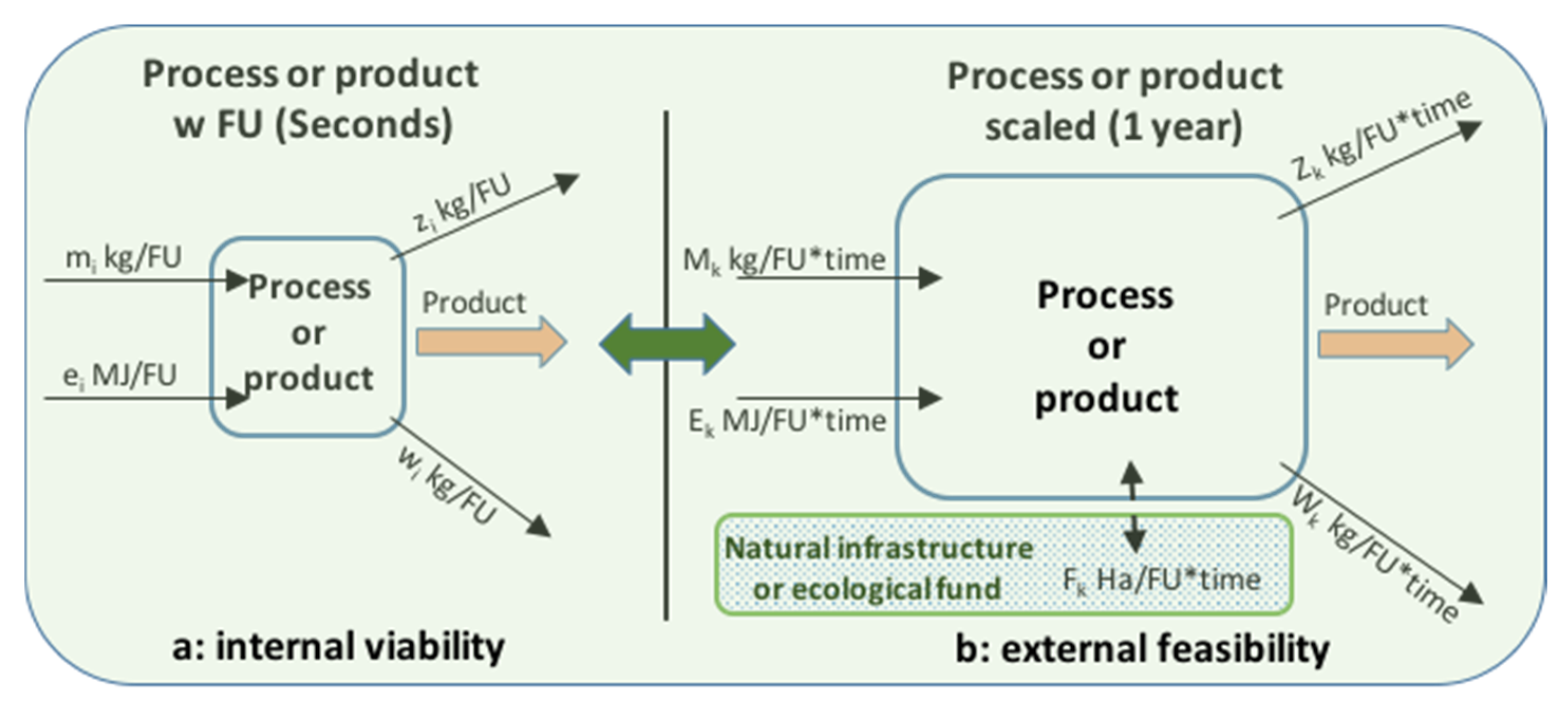
2.1. Introduction to the Principles of MuSIASEM

MuSIASEM has a theoretical framework with three key components: the FF model (economic), hierarchy theory, and the relational analysis of ecological systems, which were developed and operationalized in a toolkit through multi-level grammar instead of using models or just a black box [6,15,30]. The FF model was introduced by the bioeconomic framework of Georgescu-Roegen [14] and incorporated into the MuSIASEM. The fund elements are the production factors, such as (i) the technological capital and human activities, and (ii) the ecological funds, such as land use, aquatic and terrestrial ecosystems, atmosphere, and resources (structural elements). Flow elements are those elements that enter and leave the fund elements, such as the outputs that are generated (products or emissions) or inputs (water, energy, materials) that are consumed by the socio-economic process. Finally, the stock elements are accumulated flows that change their size over time [6]. Moreover, MuSIASEM incorporates three elements to check the sustainability of SES, the feasibility (external constraints in the biosphere), the viability (internal constraints in the technosphere), and the desirability (compatibility with normative values and societal institutions) [47,48].

2.2. MuSIASEM Principles in LCA

In the analysis, the FF model and the spatial (regional) and temporal scale (one year) elements of MuSIASEM were addressed to build the FF-LCA integrated approach. To employ this approach, stock-flows, fund–flow, and flow–flow ratios associated with a defined size and quality of fund elements of the demand side to water and fossil depletion and environmental intensity (climate change) categories on the sink side were estimated, as proposed by Mayumi and Giampietro [48] (

Table 1. Stock-flow, flow, and fund ratios considered for the scaled process to one year for water and energy depletion and climate change related categories.

Inflow Fund (Supply SIDE)	Outflow Fund (Sink SIDE)
Natural gas (PES) [m3/y]	Electricity (E) [GWh/y]
Water [m3/y]	CO2e [t/y]
O&G reserves [Mtoe]	Forest land [ha]
Land of oil and gas reserves [ha]

). Furthermore, to integrate the spatiotemporal scale in the FF-LCA approach on the supply and sink sides, the GIS and CO2FIX models [49] were considered, as shown in Figure 1 and illustrated in the following subsections.

Figure 1 illustrates and contextualizes the connections between the requirement to supply flows of material and energy for a process or PS from the technosphere and the biophysical constraints in a territory to provide ecosystem services. Further, the figure allows to understand the link between these two processes, highlighting that the changes in the EFs can only be observed on a large timescale (e.g., years, decades or centuries), which is different to the short timescale (seconds or hours) perceived by humans or the societal fund [45,47] to a large spatial scale. The forest carbon sequestration (FCS) and GIS modeling to analyze the supply and sink capacity for the ecosystem to develop this FF-LCA integrating approach were considered.

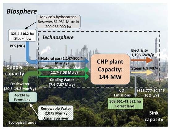
2.3. LCA Case Study: CHP w/o and wPCC Plus FCS

The LCI and LCIA data at two different time scales and three impact categories (water and fossil depletion and climate change) based on an LCA study by Morales-Mora et al. [3] were used. The CHP plant generated 1196 GWh/y of electricity as gross secondary energy carriers (GSEC) and produced emissions of 1.6 MtCO₂/y. The plant is located in the Morelos Petrochemical Complex (MPC) in the southeast of Veracruz, Mexico.

The schematic characteristic of the study cases used in the assessment is illustrated in Figure 2. Case 1 (C1) represents the CHP plant operating with a steam turbine (ST), Case 2 (C2) considers a gas turbine (GT) plus a heat recovery steam generator (HRSG), and Case 3 (C3) deals with GT+HRSG plus a post-combustion CO₂ capture (PCC) system to be utilized in urea production [3]. C1 is the state in which the CHP plant currently operates, C2 is a project that has a front-end engineering design (FEED), and C3 is a proposal built through process simulations. Figure 2c depicts the relationships between the CO₂ emissions by the CHP plant with FCS, i.e., carbon sequestration in tons, which can be translated into the area-base using sequestration rates by the forest according to the approach of Mancini et al. [50].

The assessment addressed the following aspects: (i) the requirement of material (water) and energy (PES) consumption on the supply capacity, (ii) assessment of the favorable boundary conditions on the sink capacity by the CHP plant CO₂ emissions for checking the carbon flow against spatial constraints based on the GIS analysis, and (iii) estimation of how much forest is required through the CO2FIX model so that the CHP plant can fulfill its technical and economic functions. The study is explained in terms of top-down (inflows and outflows) and bottom-up causality.

For calculation of the material and energy flows on the supply side and the relative weight of the three impact categories on the sink side, the formal process referred to FU (seconds) was addressed, as shown in Figure 3a (left). The material and energy flow inputs required to operate the CHP plant from the technosphere and the potential environmental impacts of the flows to the biosphere are shown in Figure 3a (left) according to the FU [51] and top-down model approach. The assumption made for the scaling up of the LCI and LCIA results of the CHP plant was established according to the process shown in Figure 3b (right), and subsequently, those values were calculated for one year (350 days of operations) to observe the patterns of demand for inputs and outputs instead of the flows referred to for the FU, as set out in the traditional LCA.

The assessment focuses on determining the link between the FF model in terms of the depletion of resources (water and fossil fuels), on the supply side, and the environmental impact (CO₂ emissions), on the sink side. The FF-LCA approach was coupled with the CO2FIX model and the GIS to check the availability of suitable forest land for carbon sequestration (see Figure 1) considering the ability of non-equilibrium thermodynamics to achieve their self-organizing perspective [15,52].

2.4. Requirement of Flow-Ecological Funds (Water and PES)

The CHP plant is in the Lower Uxpanapa River watershed in the State of Veracruz, Mexico. The area has an average annual rainfall of 2266 mm, a natural annual average runoff of 1991 Mm³/y, and a committed annual downstream volume of 78 Mm³/y [53]. The Costera Coatzacoalcos aquifer underlies the watershed with an average annual total recharge of approximately 172.2 Mm³/y and a committed natural discharge caused by a groundwater flow of approximately 9.7 Mm³/y [53,54,55]. Renewable water in the study area, as assessed by the volume surface and groundwater that may be sustainably allocated in the region, is approximately 2075 Mm³/y, and the water yield of the basin is approximately 10,709 m³/ha·y (

Table 2. Renewable water and water yield in the watershed where the CHP plant is located (based on DOF [53,54,55]).

Watershed	Surface [ha]	Surface Water Availability [m3/yr]	Groundwater Availability [m3/yr]	Renewable Water [m3/yr]	Water Yield [m3/ha·yr]
Lower Uxpanapa River	193,830	1,913,000,000	162,500,000	2,075,497,000	10,709
Total water allocations in the basin: 49 Mm3/yr

).

This study uses the water yield measured in m³/ha·y, to assess the area required to compensate for the impact on water depletion. As a first step, the renewable water of the basin, defined by Gleick [56] as the water that may be feasibly and sustainably used in a country, region, or watershed, was assessed based on the method established in the Mexican official standard NOM-011-CONAGUA-2015 [57].

The content of renewable water reported is the sum of the annual average volume of surface and groundwater in cubic meters per year (m³/y). According to the National Water Commission of Mexico (CONAGUA), since less than 2.3% of the renewable water is allocated, its impact on water deprivation to other users by being used in this CHP plant is negligible. Secondly, the water yield, defined as the amount of water, "produced" annually by the watershed per unit area, was calculated as the average annual volume of renewable water divided by the watershed surface in hectares (m³/ha/y) to build an indicator of the environmental intensity (flow–water/fund–land) of the surface with the natural infrastructure that is required to compensate for the water depletion impacts of the CHP process. In this study, water stress was used as a biophysical indicator to relate it to the reported value of water depletion. Commonly, it is the ratio of total annual freshwater withdrawals to the hydrological availability (WTA). Moderate and severe water stress occurs above a threshold of 40% [56].

Moreover, the fossil depletion category was analyzed as stock-flow, considering the levels of the reserve of oil and gas reported for Mexico [58]. The area of oil reserves required to supply the needs of the CHP plant was estimated using GIS from digital maps of exploration and hydrocarbon extraction [59].

2.5. Requirement of Sink Capacity (Size and Quality of the Ecological Fund to CO₂ Emissions)

Quantitative assessments of the sink capacity of the global warming category and mitigation scenarios from FCS [60] were performed using the CO2FIX model (version 2.1) and ArcGIS 10.2. Martínez-Bravo and Masera [61,62] used the CO2FIX model to estimate the amount of carbon that could be sequestered under different vegetation conditions in a carbon sequestration scenario for 60 years in Jaguaroundi Park (JaP) and Tuzandepetl Park (TzP), which are nature reserves near the CHP plant assessed in this case study. The CO2FIX model simulates carbon capture through the accumulation of carbon stocks and fluxes in forests, soils, and wood products [49]. CO2FIX is a simulation model that uses empirical yield curves [63]. The total JaP+TzP (tropical rainforests) area covers 1519 (801+718) ha and consists of mature primary and secondary forests, which provide a range of ecosystem services including carbon sequestration [64,65]. Both areas are nature reserves belonging to the government oil company PEMEX and are located around the MPC CHP plant. Secondary vegetation types present in the JaP+TzP were used to model carbon sequestration from a vegetation recovery point of view and to achieve characteristics like those of high evergreen lowland forest (mature primary forest) (

Table 3. The baseline of carbon content and capacity of carbon sequestration by forest type in Tuzandepetl and Jaguaroundi Park.

Type of Forest in Tuzandepetl (Tz) Park	Forest Land (ha)	Area Biomass (tC/ha)	Capture (tCO2/ha/yr) Average 60 Years	Capture by Coverage (tCO2/yr)	Average by Park (tCO2/ha/yr)	Total Capture (tCO2/yr)
Secondary tree vegetation	297.5	72.3	2.0	599.8
Secondary shrub vegetation	62.0	4.6	0.9	53.6
Mangrove	55.4	74.0	4.6	255.4
Grassland	304.2	2.2	0.2	60.6	1.9	969.4
Total	719.0			969.4
Jaguaroundi (Ja) Park
Secondary tree vegetation	166.0	106.0	2.4	401.8
Secondary shrub vegetation	113.0	27.0	0.8	90.6
High evergreen lowland forest	139.0	158.0	1.7	232.2
Grassland	383.0	1.5	0.4	145.4	1.3	870.0
Total	801.0			870.0		1839.4

). The parameters of the studies of JaP+TzP determined the CO₂ sequestration capacity in one hectare of vegetation.

The amount of evergreen forest was used as a target to carry out the projection for 60 years. An area of 1519 ha was defined as the JaP+TzP mitigation area for the following procedure. The annual CO₂ emissions of the CHP plant were used to estimate the equivalent JaP+TzP mitigation area of the C1 (baseline), C2, and C3 scenarios (see Figure 2). The impact of mitigation scenarios of 10%, 30%, 50%, and 100% in the forestry area was represented with the use of ArcGIS 10.2 using buffer radios for each percentage.

Another way to evaluate the impact of emissions is using the total carbon sequestration area of JaP+TzP together to calculate how many times that area is necessary to mitigate the emissions. Then, the line buffer identifies the sea area covered by the proximity of the emission sources to the coastline; the area corresponding to the sea ecosystem was discriminated. Only the terrestrial ecosystems corresponding to the municipal area of the southeast of Veracruz and Tabasco State were considered. From these results, the viability of the biomass energy with carbon capture and storage (BECCS) technology for Mexico [66] was also discussed.

Finally, the LCI and LCIA data used in this study were obtained from Morales-Mora et al. [3]. To relate the size and quality of EFs (Uxpanapa watershed, hydrocarbon reserves, and land forest) to the CHP plant, the data were obtained from the National Water Commission of Mexico (CONAGUA), National Hydrocarbon Commissions (NHC), The National Institute of Statistics and Geography (INEGI), and PEMEX databases using 2018 as the base year.

3. Results and Discussion

3.1. Spatiotemporal to One-Year Operations

Table 4. Comparison of the internal and external flow matrix of the formal process (CHP plant) for the FU (Flows/MWh) model (a) vs. the scaled CHP to 1 year (b) for the flows-EFs nexus (Adapted from Morales-Mora et al. [3]).

(a) FU Model (Time Scale: Seconds)
	Identifications	Unit	C1	C2	C3
Supply-side	External requirement inputs (LCI) (Biosphere)
Water	Water	m3	20.5	8.73	8.73
Energy (PES)	Natural gas	Nm3	1165.0	669.7	669.7
	Internal requirement inputs (LCI) (Technosphere)
	Caustic soda (50%)	kg	6.3	0.01	0.01
	Sulphuric acid (98%)	kg	5.6	0.01	0.01
	Aluminium sulphate	kg	0.7	0.001	0.001
Materials	Chlorine	kg	0.69	0.0007	0.001
	Chemical lime	kg	0	0.00	0.00012
	Condensed of comeback	t	0	3.1	0
	MEA make-up (30%)	t	0	0	0.0
Energy	Consumption electricity	kWh	0	0	75.2
Water	Cooling water make-up	m3	7.7	2.8	2.8
	Demineralization water	m3	12.8	5.9	5.9
	Outputs: products/emission (User: petrochemical plants)
Energy (EC)	Electricity	MWh	1.0	1.0	1.0
	Steam (45 kg/cm2)	t	12.8	5.8	5.8
	Steam (19 kg/cm2)	t	0.20	0.16	0.16
	Steam (4.5 kg/cm2)	t	0	0.58	0
Emissions	Flue gas (CO2)	t	1.67	1.33	0.01
	CO2 (As product by CO2 capture)	t	0	0	0.06
	Outputs: modelling environmental load (LCIA)
Total Environmental Load	Climate change	kgCO2 eq	626.0	460.0	42.0
	Ozone depletion	kg CFC-11 eq	4 × 10−7	1 × 10−7	0
	Human toxicity	kg 1,4-DB eq	0.7	0.3	37.9
	Photochemical oxidant formation	kg NMVOC	3.0	1.9	0.3
	Particulate matter formation	kg PM10 eq	1.3	0.8	0.4
	Ionising radiation	kg U235 eq	0.3	0.0	0.5
	Terrestrial acidification	kg SO2 eq	5.6	3.6	1.8
	Freshwater eutrophication	kg P eq	6 × 10−5	6 × 10−6	0.1
	Marine eutrophication	kg N eq	0.1	0.0	0.0
	Terrestrial ecotoxicity	kg 1,4-DB eq	0.0	0.0	0.0
	Freshwater ecotoxicity	kg 1,4-DB eq	0.1	0.0	2.7
	Marine ecotoxicity	kg 1,4-DB eq	0.1	0.0	0.8
	Agricultural land occupation	m2a	0.001	0	0
	Urban land occupation	m2a	0.003	0	0.1
	Natural land transformation	m2	0.000	0	0
	Water depletion	m3	1.1	0.4	1.2
	Metal depletion	kg Fe eq	0.1	0.0	0.7
	Fossil depletion	kg oil eq	161.4	104.4	83.3
Sink-side	(Environmental load to local territory or region)
	(b) Scaled Process (One Year)
	Identifications	Unit	C1	C2	C3
Supply-side	External requirement inputs (LCI) (Biosphere)
Water	Water	Mm3	20.3	14.2	14.2
Energy (PES)	Natural gas	MNm3	1148.0	801.6	800.4
	Internal requirement inputs (LCI) (Technosphere)
	Caustic soda (50%)	t	6207.1	7.42	7.4
	Sulphuric acid (98%)	t	39,842.9	38.88	38.9
	Aluminium sulphate	t	1086.8	0.951	1.0
Materials	Chlorine	t	0.0	0	0.3
	Chemical lime	t	126,259.8	96.19	0
	Condensed of comeback	Mt	0	3.7	0
	MEA make-up (30%)	t	0	0	3544
Energy	Consumption electricity	MWh	0	0	7578
Water	Cooling water make-up	Mm3	7.6	7.1	7.1
	Demineralization water	Mm3	12.7	7.1	7.1
	Outputs: products/emission (User: petrochemical plants)
Energy (EC)	Electricity	GWh	985.3	1196.4	1196
	Steam (45 kg/cm2)	Mt	7.1	6.9	6.9
	Steam (19 kg/cm2)	Mt	0.19	0.19	0.19
	Steam (4.5 kg/cm2)	Mt	0	0.6937	0
Emissions	Flue gas (CO2)	Mt	1.65	1.50	0.02
	CO2 (As product by CO2 capture)	Mt	0	0	376,250
	Outputs: modelling environmental load (LCIA)
Total Environmental Load	Climate change	t CO2 eq	616,767	550,342	50,249
	Ozone depletion	t CFC-11 eq	3.9 × 10−4	1.53 × 10−4	0
	Human toxicity	t 1,4-DB eq	661.9	364,856.9	45,343.4
	Photochemical oxidant formation	t NMVOC	2918.9	2293.2	299.1
	Particulate matter formation	t PM10 eq	1235.0	969.4	478.6
	Ionising radiation	t U235 eq	255.8	0.0	598.2
	Terrestrial acidification	t SO2 eq	5501.6	4320.1	2153.5
	Freshwater eutrophication	t P eq	0.1	0.0	59.8
	Marine eutrophication	t N eq	50.6	38.6	35.9
	Terrestrial ecotoxicity	t 1,4-DB eq	0.6	13.0	47.9
	Freshwater ecotoxicity	t 1,4-DB eq	85.2	4.2	3230.3
	Marine ecotoxicity	t 1,4-DB eq	83.7	4.0	957.1
	Agricultural land occupation	m2a	0.0	0.0	0.0
	Urban land occupation	m2a	0.0	0.0	0.1
	Natural land transformation	m2	0.0	0.0	0.0
	Water depletion	m3	1,065,826	496,352	1,435,674
	Metal depletion	t Fe eq	51.1	0.0	837.5
	Fossil depletion	t oil eq	159,068	124,852	99,660
Sink-side	(Environmental load to local territory or region)

(a,b) shows the comparison data for the two-time horizons between different amounts of inflow on the supply side (looking from the biosphere and the technosphere) and the amount of outflow on the sink capacity (the products and environmental impacts).

These different amounts of energy and material supply generate different environmental effects [33] that can be observed on the supply side and the sink side. When the FU (micro timescale) is used, there is only interest in the viability (technical and economic) of the CHP plant Table 4 (a), and less attention is paid to the changes in the feasibility assessment of the ecological resources.

This depiction allows different numbers and implications for the processor and natural system to be seen than when looking only at the normalized processor or the parameters of the formal LCA process (CHP plant) for the FU (Flows/MWh) model. In contrast, Table 4 (b) shows the result when the quantitative LCI and LCIA of the CHP plant for the three scenarios cases (C1, C2, and C3) and for other timescales are scaled up. In this case, Table 4 (b) illustrates the internal inputs required by the technosphere for the CHP plant to function and produce heat (steam) and electricity. Over one year of operation, the CHP plant produces 985–1196 GWh of electricity and 1.5–1.6 Mt of CO₂ emissions (see output products/emissions of Table 4 (b)).

The external inputs from the biosphere are 20.3 million m³ (Mm³) of water and 1147.8 million normal cubic meter (MNm³) of natural gas (NG) for baseline scenario C1. Scenarios C2 and C3 require 14.2 Mm³ of water and 800 MNm³ of NG (Table 4 (b)). It is important to note that the consumption of PES and water for scenarios C2 and C3 are similar, and this is because the role that HRSG plays in C2, which allows supplying the steam required for the CO₂ capture unit of the C3 (see Figure 2b,c). According to Morales-Mora et al. [3], in the CHP plant coupling PCC, no supplementary boiler is required to provide thermal energy for solvent regeneration to obtain CO₂-rich and regenerated solvent streams, as in the case of the natural gas combined cycle (NGCC) plant with PCC. Hence, as it is shown the Table 4 (b), the external requirement input from the biosphere, some internal material from the technosphere, and output as electricity and steam generation to CHP plant without and with PCC are almost similar. However, the potential environmental impact is different in both cases.

3.2. External Constraints: Depletion of Abiotic and Biotic Natural Resources

The degree of water stress in the Lower Uxpanapa River watershed is low (Table 2) since approximately 2.3% of the total renewable water [53] in the basin is allocated. In this case, since the watershed has plenty of water available, there are no external natural infrastructure constraints. However, it is essential to highlight that the 14.2–20.3 Mm³/y of water allocated to the CHP plant represents 29%–41% of all water allocation in the watershed.

Evaporation, transpiration, and integration into a product or release into a different drainage basin or the sea are the primary reasons for water consumption [67]. Non-consumptive water use refers to the water that remains in or is immediately returned to the location in a stream from which it was extracted, such as that used in hydroelectric power generation and water cooling. From the 14.2–20.3 Mm³/y of water allocated to the CHP process (Table 4 (b)), only 14% is considered consumptive in scenario C1, 7% in C2, and 20% in C3 (from Table 2).

It is known that watersheds represent vital natural infrastructure that collect, store, and filter water and provide benefits for biodiversity conservation, climate change adaptation and mitigation, food, water, and energy security [66]. It is essential to consider industrial production activities in early planning strategies (since the location of the facilities is decided upon) to protect the water sources that the people, nature, and industrial processes depend on to achieve sustainable development. Natural ecosystems located in the Uxpanapa watershed, such as forests and wetlands, provide essential hydrological and ecosystem services (from water flow regulation and flood control to water purification and carbon sequestration). To ensure these ecosystem functions and associated benefits continue, they should be assessed within the LCA methodology. The water yield rate proposed in this study provides an accurate measure of the size of the potential impact on the natural infrastructure (measured in hectares), and it is interpreted as the area of essential infrastructure that must be conserved and restored to compensate for the water consumed in the CHP process.

Table 5. Water depletion and water yield in the watershed in the study area.

Water Depletion [m3/y]				Water Depletion/Water Yield Ratio (Hectares)
Unit	C1	C2	C3	Unit	C1	C2	C3
FU	1.082	0.415	1.2	-	-	-	-
1 year	1,065,826	496,352	1,435,674	1 year	95.5	46.4	134.1

shows the water depletion category (left) estimated with the ReCiPe method [3], which refers to the sum of the volume of consumptive water use of the LCI in m³.

There is a difference of 3–4 orders of magnitude in the water used by the CHP plant between the timescale referred to in the FU, and the process scaled up to one year of operation. In this way, the metabolic patterns of the CHP plant concerning the biophysical constraints of the territory which could not be perceived and analyzed in the FU model can be observed. The water depletion/water yield ratio for each case on the right side of Table 5 is shown.

The CHP plant requires 46.4–134.5 ha or a local ecological fund (Uxpanapa river) to supply fresh water for a year. In this case, there is lower pressure over the Uxpanapa watershed because the higher water yield in the basin is associated with the higher annual rainfall in the area.

The annually estimated water yield concept has a number of limitations: (i) It is based on annual averages, which neglect extremes and do not consider the temporal dimensions of the water supply; (ii) the concept does not consider the spatial distribution of land use/land cover; (iii) the concept does not consider sub-annual patterns of water delivery timing; and (iv) the model greatly simplifies consumptive demand and supply by distributing it over the landscape. Hence, modeling the temporal and local patterns of overland flow requires detailed data that are not available or appropriate for our approach. Even so, this concept provides a useful initial assessment of how much area is required to compensate for water consumption in a specific watershed.

As can be seen, the impacts on abiotic resources of scaling the process to 1 year of operation would be 0.159 Mt oil/y for scenario C1, 0.124 Mt oil/y for scenario C2, and 0.099 Mt oil/y for scenario C3 as fossil depletion or 1148 million Nm³ of NG for C1 and 800 Mm³, on average, for C2 and C3 as the requirement of PES of the CHP plant (Table 4 (b)). If the PES requirements for the CHP plant, according to the data shown in Table 4 (b), are compared with the 1P hydrocarbon reserves [58], the impact of scenario C1 on the total reserves for Mexico would only be 0.0019%. Also, a contribution of only 0.0003% for the NG reserves in m³ billion was estimated (

Table 6. Mexico’s hydrocarbon and NG reserves ^a and fund–flow ratio of the CHP plant.

Total Hydrocarbon Reserves b (Mtoileq)			NG Reserves (m3 × 109)
1P d (90%)	2P d (50%)	3P d (10%)	1P d (90%)	2P d (50%)	3P d (10%)
61,931	117,982	185,907	353,898	684,248	1,060,042
Total reserve [PJ]			NG reserve [PJ]
98,944	722,292	98,944	722,292	98,944	722,292
Reserve-oil extraction (R/E) ratio d (Years) e			Reserve gas extraction (years)
8.5	16.1	8.5	16.1	8.5	16.1
Fund–flow ratio (Ha reserve) to CHP plant (fossil fuel depletion category)
C1	C2	C3
516.2	405.1	323.4

Source: ^a: According to the Petroleum Resources Management System; ^b–d: PEMEX-NHC [58]; 1P: Low-Media: 2P: High; 3P: Very high uncertainty; ^e: with respect to 1 January 2018.

).

From a spatial point of view, the Mexican hydrocarbon reserves (stock-flow) are in an area of 200,965,000 ha [59], which includes offshore and onshore land and represents only 0.39% of the national territory. For 1P reserves, a value of 0.0032 ha/toe is estimated. From this reference value and considering the estimation of fossil fuel depletion, the CHP plant would require 516.2 ha for C1, 405.1 ha for C2, and 323.4 ha for C3 to cover its annual demand of PES for one year of operation at the local scale (Table 6). From a local scale point of view, for this energetic system, those values represent a low pressure on the environment.

However, on a national scale, Mexico only has hydrocarbon 1P reserves for 8.5 more years, (Table 6), which is a short time as fossil fuels provide fuel for most of the country. Thus, this period of reserves could be reduced due to an increase in PES consumption to generate more EC. Particularly, for this abiotic resource, Mexico has external biophysical constraints, which are related to the overall size of the energy flow requirement of the country [68].

For instance, the country imports 8 billion ft³/d of NG, which represents 85% of its consumption. Of that amount, the Mexican oil and gas industry (PEMEX) demands 2 billion ft³/d, and the remaining 6 billion is used by the electricity sector, industry, and personal residences [69].

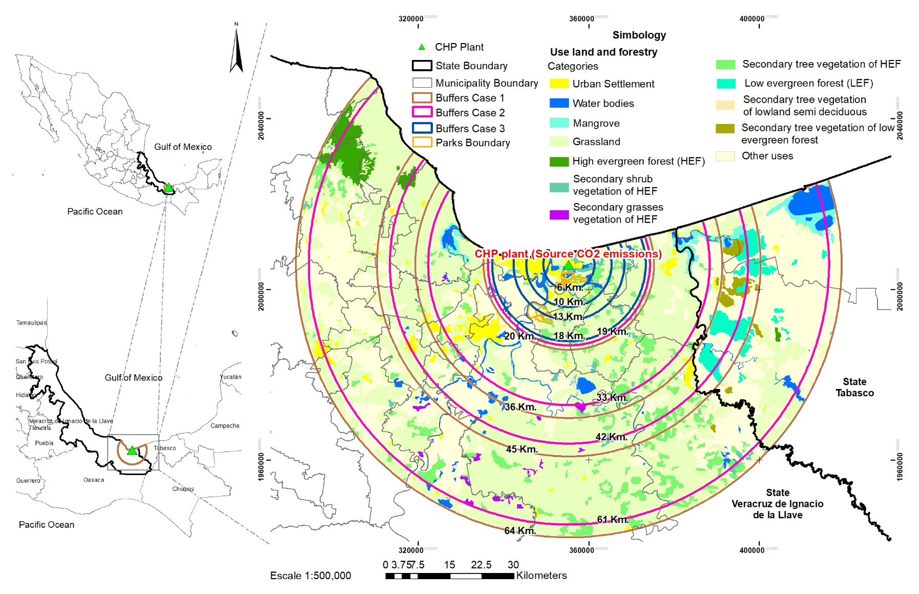
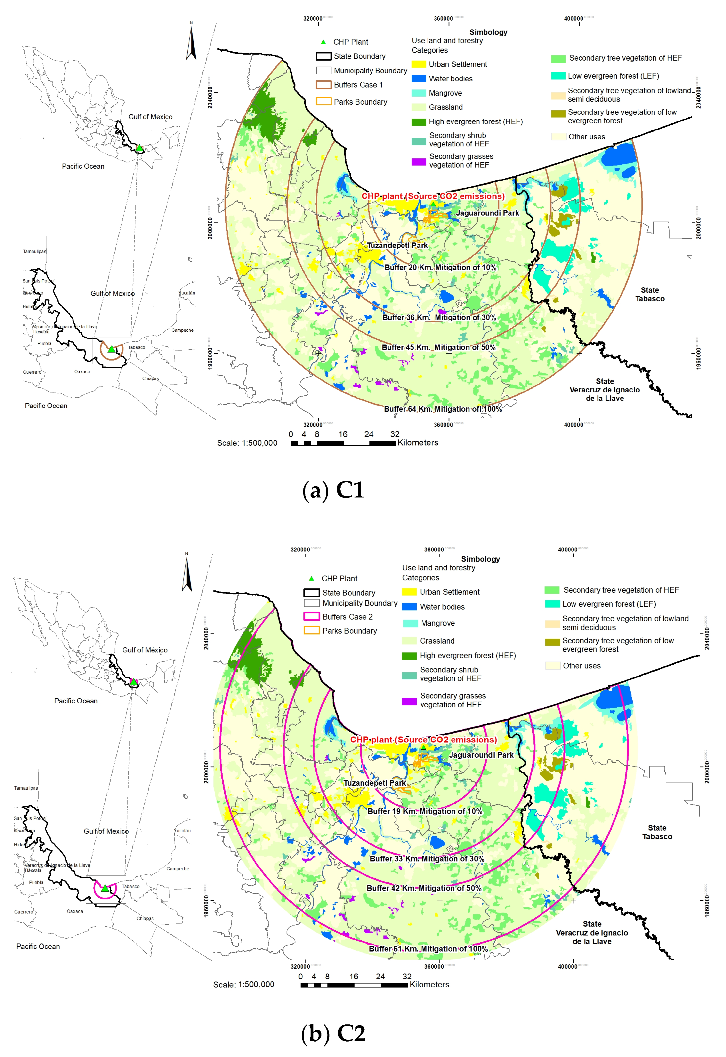
3.3. Sink Capacity: Modelling CO₂ Emissions and FCS

Concerning the environmental effects on the sink side, the climate changes category shows results with a more important impact than all midpoint categories with 0.616 MtCO_2e/y for scenario C1, 0.55 MtCO_2e/y for scenario C2, and 0.052 MtCO_2e/y for scenario C3 (Table 4 (b)). These numbers are significant because now there is information and data about the sources of CO₂ emissions at other time scales. The baseline of carbon (C) shows that JaP+TzP has a store from 1.5 to 158 tC/ha in different vegetation types (Table 3). The maximum carbon stored in vegetation (158 tC/ha) occurs in high evergreen lowland forest (HELF). These data represent the carbon maximum in scenarios of carbon fixing when all vegetation types have similar HELF conditions. Pompa-García and Cigala-Rodríguez [70] identified an average carbon stock of 106.9 tC/ha in the rainforest of Mexico. The average CO₂ captured annually by the vegetation of each park was 870.0 tCO₂/y in JaP (801 ha), and 969.4 tCO₂/y in TzP (719 ha). Table 3 shows that the average carbon sequestration by the forests in the park was 1.9 tCO₂/ha/y for TzP and 1.3 tCO₂/ha/y for JaP. The two parks together had average carbon sequestration of 1.6 tCO₂/ha/y; the world average is 0.73 ± 0.37 tCO₂/ha/y [50].

Table 7. Potential FCS (tCO₂/ha) for four sceneries and area projected (left), and its equivalent area to the number of parks (right) necessary to mitigate CHP plant emissions scaled to one year.

Scenario (Mitigation)	C1 (Baseline)	C2	C3	C1 (Baseline)	C2	C3
	Forest Land [ha]			Num. of Parks (Tz-Ja) as Conservation Areas
10%	509,65	45,476	4152	27.7	24.7	2.3
30%	152,895	136,428	12,456	83.1	74.2	6.8
50%	254,825	227,381	20,760	138.5	123.6	11.3
100%	509,651	454,762	41,522	277.1	247.2	22.6
CO2e emissions [t]	616,766	550,342	50,249

shows the potential FCS for four scenarios of CO₂ mitigation. Levels of (a) 10%, (b) 30%, (c) 50%, and (d) 100% for the CHP plant regarding the projected forest land (left), parks (right), or sink capacity required to mitigate such emissions were estimated. As we can see, to achieve 100% CO_2e mitigation, the base case (C1) required 509,766 ha or equivalent to 277.1 JaP+TzP to carry out FCS.

In contrast, the C3 which, from a technological point of view, is the option with fewer emissions considering the PCC (see Figure 2c), requires 41,525.8 ha and only 22.6 parks, equivalent to a reduction in the area of the natural sink of 92% for C1. Our data show a strict relation between funds (forest land) and flow (CO₂ emissions). The specific spatial area in Figure 4 is shown. The GIS data show the area around the CHP plant for each mitigation percentage scenario for C1, C2, and C3, which summarizes the fund–flow ratio (ha/tCO_2e) (see Table 1). That is, the ecological fund mitigates the CO₂ emissions of the CHP plant. C1 is a business scenario. The spatial modeling for the four scenarios was integrated into Figure 4.

The buffers refer to spatially explicit modeling to show the impact on land area in each case. The results show a requirement of 509,651 ha (Table 7) or a maximum achieved buffer radius of 64 km from CHP for 100% carbon sequestration in C1 during a year, which covers the southeastern area of Veracruz State and the northeastern area of Tabasco State. From a feasibility assessment point of view, even though that JaP+TzP has a carbon storage rate of 33% higher than the national average [60], the data show that they have a deficient capacity to act as carbon sinks and carry out sequestration of the CHP emissions.

In other words, external biophysical constraints on the sink side of those regions have been identified. In this sense, the ecosystems need significantly more secondary vegetation growth per hectare to carry out carbon sequestration, which is subordinate to the given stage of the Holling adaptive cycle in which the ecological system is located [71]. According to these phases, changing conditions of the forest by natural or anthropogenic disturbance, the carbon sequestration also changes. Nevertheless, despite this very low carbon sequestration, the local forests contribute to reducing the greenhouse effect and climate change.

Figure 5 shows the detail of the spatial modeling that was used to evaluate the forest ecosystem’s capacity to sequester carbon for each case and its four mitigation scenarios.

The alternative case, C3, reduces the area of emissions impact, needing 4152 ha to mitigate 10% and 41,522 ha to mitigate all emissions during a year (Figure 5c). This is equivalent to 2.3 times and 22.6 times the area of JaP+TzP, respectively (Table 7). From the source of emissions (i.e., the CHP plant) in the direction from north to south, the buffer extends for 18 km (Figure 5c).

Regarding the spatial results, it is interesting to assess the potential of BECCS technology for the biomass transformation of C4 plants (e.g., sugar cane, maize). BECCS is considered to be a negative emissions technology that is used to remove CO₂ from the atmosphere [72], and it has been considered a keystone technology for delivering the Paris Agreement on climate change [73,74]. However, the conversion of native vegetation to the agricultural production of sugar cane and maize to produce biofuels can reduce the net primary production, because C4 plants have a carbon storage lifetime of fewer than six months, and displace natural ecosystems [13]. According to Gomiero [75], biofuel production may cause an increase in net CO₂ emissions.

From an economic point of view, within the mitigation options for the target of 1.5 °C, the latest Intergovernmental Panel on Climate Change (IPCC) report [76] considers not only the post-combustion CO₂ capture with a cost of 30–60 USD/t CO₂ captured [25], but also the removal of CO₂ from our atmosphere by direct air capture (DAC) technology with a cost of 94–232 USD/tCO₂ captured [77]. In contrast, Busch et al. [78] estimate that the removal from tropical reforestation between 2020 and 2050 could be up to 20 USD/tCO₂. That means forest restoration is cost-effective but limited in time compared to the technological options. Instead, BECCS has CO₂ emission associated with the biomass generation (sugar cane, maize, oil crops) for the electricity generation process. Overall, biomass production to supply BECCS could be a constraint, such as the availability of land or water [72]. For instance, García et al. [79] estimated a carbon footprint of sugar production in Mexico of 450 to 630 kgCO₂/t sugar, corresponding to 265 to 466 kgCO₂/t sugar at the agricultural stage. Additionally, BECCS would require subsidies for the crops of biomass and higher costs due to the lack of infrastructure (pipeline networks) in the areas of crops, energy generation, and geological storage [66]. In this sense, some organizations, such as the Global Capture Storage Institution, promote the BECCS in developing countries [73]. However, it should be considered that many territories have a strict set of biophysical constraints in terms of the feasibility of using natural resources. According to the Special Climate Change Program (PECC 2014–2018), 319 municipalities in Mexico (13% of the total) present greater vulnerability to the impacts of climate change, in particular, droughts and floods. The climate change scenarios for the period 2015–2039 estimate that the annual temperature will be 2 °C higher in the North, while in the rest of the territory, it has been estimated to increase by between 1 and 1.5 °C. In general, rainfall decreases by 10% to 20% [80].

In this sense, if comparing the emissions of C3 with the FCS by the Ja+Tz parks (1519 ha), mitigation in one year only be 3.6% (Figure 6). This basic design of C3 plus FCS could be considered as a proxy of BECCS technology and, therefore, its performance in Mexico. Also, in a similar study, Meza-Palacios et al. [81] found that the sugarcane growth and harvesting stage provides the most harmful environmental impact (52%) followed by electricity cogeneration (25.7%) from bagasse.

This means, as stated by Gomiero [75], that BECSS would have net CO₂ emissions and require extensive forest land area to mitigate the reduced percentage of CO₂ generated by the hypercycle of the energy system.

Moreover, BECCS would compete with the crop land–water destined to cover the permanent food demand for human consumption. This is important because there is biophysical and biogeochemical feedback due to the impact of climate change on forest land and vice versa [82]. With respect to the energy density per square meter (W/m²) or power density (PD), the NG provides 200–2000 W/m², whereas the liquid biofuel has a very low PD (0.45 W/m² on average) and takes too much land to try to replace fossil fuels [75,83].

3.4. The Usefulness of the WEC Nexus as a Flow–Fund Ratio and Fund Size in LCA

Table 8. Environmental intensity ratios of the CHP plant.

Fund–Flow and Flow–Fund Ratios	Unit	C1	C2	C3
Forest land req	ha	509,651	454,762	41,522
CO2e	t	616,766	550,342	50,249
	Ratio ha-t	0.83	0.83	0.83
Electricity (EC)	MW	985,250	1,196,395	1,196,395
	Ratio MW-ha	1.9	2.6	29
	kgCO2e/MWh [3]	626	460	42

shows the values of the flow–fund ratio related to the capacity of the regional ecosystem to sequester carbon in the 100% mitigation scenario and C1, C2, and C3.

A value of 0.83 ha/tCO_2e was found to be a requirement of forest land, i.e., as net uptake of anthropogenic CO₂ emissions. In this case, the net balance of carbon emissions is positive, which can be considered a benchmark for the local ecosystem’s metabolic pattern. In this sense, taking the most extensive use of forest land for CO₂ sequestration as a reference, the C1 scenario generates 1.9 MW/ha, whereas the C3 scenario generates 29 MW/ha, based on FCS. This means that the CHP plant plus PCC technology generates more electricity and steam with less use of ecological resources and fewer emissions (Table 8). Nevertheless, this ratio found could increase or decrease following actions taken to conserve or restore the land forest. As land degrades, the CO₂ sequestration and land productivity capacity also are reduced. This positive feedback increases the concentration of GHG in the atmosphere and aggravates climate change [82], again leading to further forest degradation forced by technologies such as BECCS due to competition for land and other resources.

On the other hand,

Table 9. Matrix of the WEC nexus on the supply side and sink side (biosphere) for the one-year operation of the CHP plant for each case (technosphere).

Flow Requirement	Fund Size	Unit	C1	C2	C3
Water depletion		m3	1,065,826	496,352	1,435,674
	Forest land	ha	99.5	46.4	134.1
Fossil depletion a		t oileq	159,068	124,852	99,660
	Stock land	ha	516	405	323
Climate change		tCO2eq/y	616,766	550,342	50,249
	Forest land	ha	509,651	454,762.4	41,522
Electricity		MWh	985,250	1,196,395	1,196,395
	Forest land	MW/ha	1.9	2.6	29

^a: 0.0032 ha/toe to 1P reserves.

summarizes the requirement of the ecological fund to operate the CHP plant for one year for each case. The WEC nexus with the ecological fund is necessary for the CHP plant to fulfill its function, i.e., generate 1196 GWh/yr. However, when a PS is analyzed through FU in LCA, the nexus flow–fund ecological aspect is missed. Unfortunately, these two elements are not integrated into LCA and still operate independently of each other. Moreover, when the process is scaled, and the FF model is considered, it is possible to see different spatial and temporal scale relations between the demand side for the CHP plant of water, PES, and the environmental impacts on the sink capacity by the EFs, connecting the internal view (technosphere) with the external view of the ecosystem (biosphere).

The flow–fund ratios, shown in Table 9, allow to obtain the size and quality of ecosystems, which depend on the existence of favorable boundary conditions in a territory to supply ecosystem services, to be identified. This consideration is important because the EFs require a dynamic budget or hypercycle to carry out their metabolism [46,47] to continue with the function of the supply of ecosystem services. With this data, there is now a threshold area concerning the ecological funds that the CHP plant requires to operate and fulfill its function of supplying electricity and steam to its users. The current result of traditional LCA does not provide a feasibility assessment to connect the ratios between the supply–demand–sink capacities, which should be considered in a sustainability context [84].

In this sense, this proposal differs from another emerging approach that considers the ecosystem services issue in LCA [85,86,87], but it is subordinate to the FU model, as it excludes the metabolic patterns of the consumption and environmental load of the process on other time scales. Moreover, the proposed emerging approach does not provide flow data to determine whether the metabolic patterns of PS can affect (how and why) the biophysical constraints under which a local territory may have to provide ecosystem services. For instance, the TES-LCA protocol [85] only takes into account the FU linking with the ecosystem services at a global scale but does not connect the demand (how much) for materials and energy for a PS. On this matter, a new approach by Sohn et al. [88] that combined territorial metabolism and life cycle assessment (TM-LCA) methods is introduced, which includes a regional-scale environmental impact assessment, but without considering the quantification of the ecosystem services required by the processes in territory where it is established.

Overall, Figure 7 shows the FF-LCA integrated approach, allowing the internal (technological viability) and external (biophysical feasibility) views of a CHP plant to relate to the favorable boundary conditions of the ecosystem to carry out sustainability (viability and feasibility) analyses.

The CHP plant requires EFs to be estimated in hectares to cover their demand for inputs (freshwater and NG) and to mitigate CO₂ emissions over one year of operation. Figure 7 shows the simultaneous use of internal (black box) and external views, i.e., compatibility, with external constraints.

Therefore, this approach allows the identity of energy systems to be defined as a whole, whereas by using the black box with the PS, it is not possible to perceive and represent the WEC nexus with EFs. A set of relations between societal fund (CHP plant) and the ecological funds can be visualized (see Figure 1), which allows us to understand how these different numbers are correlated to assess their impact on ecosystem services in local territories [89]. In other words, this means getting a set of categories (flow–fund ratios) that reflect the mix of functional (e.g., gas processing, generation power, ecosystem metabolism) and structural (technological infrastructure, ecological funds) elements required for the self-reproduction of the energy system [84].

With respect to the protection areas in LCA, i.e., natural resources, which protect the support of the ecosystem at the superior hierarchical level, the reality is simplified for the use of an indicator of causality, such that it does not have any meaning within their context.

Concerning the usefulness of this proposal, this FF-LCA integrated approach can be applied to build regional scenarios by using water, PES, and emissions for energy clusters of the O&G sector or industrial parks to assess the biophysical constraints of a region to supply ecosystem services.

On the other hand, currently, the sustainability programs of the companies integrate risk assessment and the environmental footprint to respond to the requirements of stakeholders and rating agencies [89,90]. The measurement of a PS with this approach, which is associated with mitigation and/or compensation measures, helps private and public organizations (e.g., Mexican electricity and O&G sector) to strengthen their adaptation and/or mitigation commitments for the intended nationally determined contribution (INDC). For 2015, Mexico’s GHG emissions were 683 MtCO_2e, of which 21.6% (148 MtCO_2e) were sequestered by forests [81]. This means that Mexico has an average as FCS of 0.75 tCO₂/, which is similar to t reported by Mancini [50] of 0.73 tCO₂/ha for forest ecosystems at the world level.

In this sense, the Mexican goal has established the unconditioned reduction of 22% of their emissions of greenhouse gases (GHG) by 2030, which means a reduction in GHG of around 210 Mt [91].

Since the intention to measure the environmental impact of a process is to identify measures to reduce them, the approach of this research is not intended to be another impact category like the ecological footprint indicator, but rather, a tool to define specific mitigation solutions associated with the area of EFs that should be under conservation actions to compensate for the potential impacts of water scarcity and climate change.

4. Conclusions

We have presented a practical approach using a relational analysis, scale inventory, and environmental impact for the one-year operation (at least) of a CHP with and without PCC to understand the implications of the flow–fund relations of the ecosystem on the demand side and the sink, which have so far been excluded from the traditional LCA. The pressure on both sides on the non-renewable and renewable resources was discussed in spatiotemporal terms to understand the implications across different scales and dimensions.

The time scale and EFs were considered for LCA improvement. For this energy system, the EFs for the WEC nexus were identified. This is an area that is required to supply water and PES and to mitigate the evaluated impacts. The suggested approach of linking FF-LCA with each type of environmental impact has strengths as well as limitations (e.g., measuring EFs by importations). Also, it requires the availability of data about ecosystem services on the supply and sinks side and for the needs of their metabolism. However, this work considered that the analytical framework allows for the contextualization and recognition of the need to assess the LCI and LCIA with the local ecosystem capacities to improve the use of LCA. Other methods provide a single indicator of the human/technological demands on nature to measure the absolute environmental sustainability.

In contrast, the approach of this work was constructed to detect which flows are making an impact on particular EFs to check whether the demand side and environmental load are compatible with such funds. It was demonstrated that linking the requirements among flows and EFs to identify biophysical constraints to a PS should be considered in the guidelines for LCA to assess whether a product or process is ecologically efficient. Also, this approach is a useful proxy or threshold for analyzing whether the PS is based on imports of material and energy flow from other regions, i.e., other ecological funds, or to determine whether the PS has enough EFs to fulfill its function.

References

1. Motazedi, K.; Abella, J.P.; Bergerso, J.A. Techno-Economic Evaluation of Technologies to Mitigate Greenhouse Gas Emissions at North American Refineries. Environ. Sci. Technol. 2017, 51, 1918–1928. [Google Scholar] [CrossRef]
2. Mexico’s Ministry of Energy (SENER). Programa de Desarrollo del Sector Eléctrico Nacional 2019–2033. Gobierno de México. 2018. Available online: https://www.gob.mx/sener/documentos/prodesen-2019-2033 (accessed on 30 July 2019). (In Spanish).
3. Morales-Mora, M.A.; Pretelín Vergara, C.; Martínez-Delgadillo, S.A.; Iuga, C.; Nolasco-Hipólito, C. Environmental assessment of a combined heat and power (CHP) plant configuration proposal with post-combustion CO2 capture for the Mexican oil and gas industry. Clean Technol. Environ. Policy 2019, 21, 213–226. [Google Scholar] [CrossRef]
4. Mekonnen, M.M.; Hoekstra, A.Y. Four billion people facing severe water scarcity. Sci. Adv. 2016, 2, e1500323. [Google Scholar] [CrossRef] [Green Version]
5. Escalante-Sandoval, C.; Nuñez-Garcia, P. Meteorological drought features in northern and northwestern parts of Mexico under different climate change scenarios. J. Arid Land 2017, 9, 65–75. [Google Scholar] [CrossRef] [Green Version]
6. Giampietro, M.; Aspinall, R.J.; Bukkens, S.G.F.; Benalcazar, J.C.; Diaz-Maurin, F.; Flammini, A.; Tiziano Gomiero, T.; Zora Kovacic, Z.; Madrid, C.; Ramos-Martín, J.; et al. An Innovative Accounting Framework for the Food-Energy-Water Nexus—Application of the MuSIASEM Approach to Three Case Studies; Environment and Natural Resources; Working Paper No.56; Food and Agriculture Organization: Rome, Italy, 2013. [Google Scholar]
7. Endo, A.; Tsurita, I.; Burnett, K.; Orencio, P.M. A review of the current state of research on the water, energy, and food nexus. J. Hydrol. Reg. Stud. 2017, 11, 20–30. [Google Scholar] [CrossRef] [Green Version]
8. Liu, Y.; Chen, W.Q.; Lin, T.; Gao, L. How Spatial Analysis Can Help Enhance Material Stocks and Flows Analysis? Resources 2019, 8, 46. [Google Scholar] [CrossRef] [Green Version]
9. Giampietro, M.; Saltelli, A. Footprint to nowhere. Ecol. Indic. 2014, 46, 610–621. [Google Scholar] [CrossRef]
10. Galli, A.; Giampietro, M.; Goldfingerd, S.; Lazarusd, E.; Lind, D.; Saltellie, A.; Wackernageld, M.; Müllerf, F. Questioning the Ecological Footprint. Ecol. Indic. 2016, 69, 224–232. [Google Scholar] [CrossRef]
11. FAO. The Water-Energy-Food Nexus. A New Approach in Support of Food Security and Sustainable Agricultura. 2014. Available online: http://www.fao.org/3/a-bl496e.pdf (accessed on 22 May 2019).
12. United Nations World Water Assessment Programme/UN-Water (WWAP). The United Nations World Water Development Report 2018: Nature-Based Solutions for Water; UNESCO: Paris, France, 2018; Available online: https://reliefweb.int/sites/reliefweb.int/files/resources/261424e.pdf (accessed on 13 June 2019).
13. The Nature Conservancy (TNC). Beyond the Source: The Environmental, Economic and Community Benefits of Source Water Protection; The Nature Conservancy: Arlington, VA, USA, 2017; Available online: https://www.nature.org/content/dam/tnc/nature/en/documents/Beyond_The_Source_Full_Report_FinalV4.pdf (accessed on 10 May 2019).
14. Georgescu-Roegen, N. The Entropy Law and the Economic Process; Harvard University Press: Cambridge, MA, USA, 1971. [Google Scholar]
15. Giampietro, M. On the Circular Bioeconomy and Decoupling: Implications for Sustainable Growth. Ecol. Econ. 2019, 162, 143–156. [Google Scholar] [CrossRef]
16. Lomas, P.L.; Giampietro, M. Environmental accounting for ecosystem conservation: Linking societal and ecosystem metabolisms. Ecol. Model. 2017, 346, 10–19. [Google Scholar] [CrossRef] [Green Version]
17. International Energy Agency. Energy Policies beyond IEA Countries—Mexico 2017. Available online: https://webstore.iea.org/energy-policies-beyond-iea-countries-mexico-2017 (accessed on 20 July 2019).
18. Rodríguez-Martínez, A.; Lechón, Y.; Cabal, H.; Castrejón, D.; Flores, M.P.; Romero, R.J. Consequences of the National Energy Strategy in the Mexican Energy System: Analyzing Strategic Indicators with an Optimization Energy Model. Energies 2018, 11, 2837. [Google Scholar] [CrossRef] [Green Version]
19. Petroleos Mexicanos. Pemex’s Business Plant 2019–2023. Gobierno de Mexico. 2019. Available online: https://www.pemex.com/en/press_room/press_releases/Paginas/2019-034-national.aspx (accessed on 20 July 2019).
20. IEA. Energy Policies beyond IEA Countries-Mexico 2017. Available online: https://webstore.iea.org/energy-policies-beyond-iea-countries-mexico-2017 (accessed on 18 June 2019).
21. IPCC. Climate Change 2014: Mitigation of Climate Change. Working Group II Contribution to the IPCC 5th Assessment Report Changes to the Underlying Scientific/Technical Assessment, 101p. Available online: https://www.ipcc.ch/report/ar5/syr/ (accessed on 5 May 2019).
22. Global CCS Institute. The Global Status of CCS Report 2018. Available online: https://www.globalccsinstitute.com/ (accessed on 18 June 2019).
23. Hassiba, R.J.; Al-Mohannadi, D.M.; Linke, P. Carbon dioxide and heat integration of industrial parks. J Clean Prod. 2017, 155, 47–56. [Google Scholar] [CrossRef]
24. Wang, M.; Oko, E. Special issue on carbon capture in the context of carbon capture, utilisation and storage (CCUS). Int. J. Coal Sci. Technol. 2017, 4, 1–4. [Google Scholar] [CrossRef] [Green Version]
25. Rubin, E.S.; Davison, J.E.; Herzog, H.J. The cost of CO2 capture and storage. Int. J. Greenh. Gas Control 2015, 40, 378–400. [Google Scholar] [CrossRef]
26. MacDowell, N.; Fennell, P.S.; Shah, N.; Maitland, G.C. The role of CO2 capture and utilization in mitigating climate change. Nat. Clim. Chang. 2017, 7, 243–249. [Google Scholar] [CrossRef] [Green Version]
27. Armstrong, K.; Styring, P. Assessing the potential of utilization and storage strategies for post-combustion CO2 emissions reductions. Front. Energy Res. 2015, 3, 8. [Google Scholar] [CrossRef] [Green Version]
28. Li, J.; Hou, Y.; Wang, P.; Yang, B.A. Review of Carbon Capture and Storage Project Investment and Operational Decision-Making Based on Bibliometrics. Energies 2019, 12, 23. [Google Scholar] [CrossRef] [Green Version]
29. Dai, J.; Wu, S.; Han, G.; Weinberg, J.; Xie, X.; Wu, X.; Song, X.; Jia, B.; Xue, W.; Yang, Q. Water-energy nexus: A review of methods and tools for macro-assessment. Appl. Energy 2018, 210, 393–408. [Google Scholar] [CrossRef]
30. Giampietro, M.; Mayumi, K.; Rámos-Martín, J. Multi-scale integrated analysis of societal and ecosystem metabolism (MuSIASEM): Theoretical concepts and basic rationale. Energy 2009, 34, 313–322. [Google Scholar] [CrossRef]
31. Mannan, M.; Al-Ansari, T.; Mackey, H.R.; Al-Ghamdi, S.G. Quantifying the energy, water and food nexus: A review of the latest developments based on life-cycle assessment. J. Clean. Prod. 2018, 193, 300–314. [Google Scholar] [CrossRef]
32. Karabulut, A.A.; Eleonora Crenna, E.; Sala, S.; Udias, A. A proposal for integration of the ecosystem-water-food-land-energy (EWFLE) nexus concept into life cycle assessment: A synthesis matrix system for food security. J. Clean. Prod. 2018, 172, 3874–3889. [Google Scholar] [CrossRef]
33. Liu, X.; Bakshi, B.R. Ecosystem Services in Life Cycle Assessment while Encouraging Techno-Ecological Synergies. J. Ind. Ecol. 2018, 23, 2. [Google Scholar] [CrossRef]
34. Moltesen, A.; Bjørn, A. LCA and Sustainability. In Life Cycle Assessment: Theory and Practice; Hauschild, M.Z., Rosenbaum, R.K., Olsen, S.I., Eds.; Springer: Berlin, Germany, 2018; pp. 59–66. [Google Scholar] [CrossRef]
35. Hellweg, S.; i Canals, L.M. Emerging approaches, challenges and opportunities in life cycle assessment. Science 2014, 344, 1109–1113. [Google Scholar] [CrossRef] [PubMed]
36. Bjørn, A.; Owsianiak, M.; Laurent, A.; Olsen, S.I.; Corona, A.; Hauschild, M.Z. Scope Definition. In Life Cycle Assessment: Theory and Practice; Hauschild, M.Z., Rosenbaum, R.K., Olsen, S.I., Eds.; Springer: Berlin, Germany, 2018; pp. 75–116. [Google Scholar] [CrossRef]
37. ISO 14040. Environmental Management—Life Cycle Assessment—Principles and Framework, 2nd ed.; ISO: Geneva, Switzerland, 2006. [Google Scholar]
38. Dyckhoff, H.; Kasah, T. Time Horizon and Dominance in Dynamic Life Cycle Assessment. J. Ind. Ecol. 2014, 18, 799–808. [Google Scholar] [CrossRef]
39. Hauschild, M.Z. Introduction to LCA Methodology. In Life Cycle Assessment: Theory and Practice; Hauschild, M.Z., Rosenbaum, R.K., Olsen, S.I., Eds.; Springer: Berlin, Germany, 2018; pp. 75–116. [Google Scholar]
40. de Haes, H.A. Life-Cycle Assessment and the Use of Broad Indicators. J. Ind. Ecol. 2006, 10, 5–7. [Google Scholar] [CrossRef]
41. Ryberg, M.W.; Owsianiaka, M.; Richardsonb, K.; Hauschild, M.Z. Development of a life-cycle impact assessment methodology linked to the Planetary Boundaries framework. Ecol. Indic. 2018, 88, 250–262. [Google Scholar] [CrossRef] [Green Version]
42. Yang, Y.; Zheng, H.; Kong, L.; Huang, B.; Xu, W.; Ouyang, Z. Mapping ecosystem services bundles to detect high- and low-value ecosystem services areas for land use management. J. Clean. Prod. 2019, 225, 11–17. [Google Scholar] [CrossRef]
43. Maier, M.; Mueller, M.; Yan, X. Introducing a localised spatio-temporal LCI method with wheat production as exploratory case study. J. Clean. Prod. 2017, 140, 492–501. [Google Scholar] [CrossRef] [Green Version]
44. Pavan, A.L.R.; Ometto, A.R. Ecosystem Services in Life Cycle Assessment: A novel conceptual framework for soil. Sci. Total Environ. 2018, 643, 1337–1347. [Google Scholar] [CrossRef]
45. Rosen, R. Life Itself: A Comprehensive Inquiry into the Nature, Origin, and Fabrication of Life; Columbia University Press: New York, NY, USA, 1991. [Google Scholar]
46. Giampietro, M. Perception and Representation of the Resource Nexus at the Interface between Society and the Natural Environment. Sustainability 2018, 10, 2545. [Google Scholar] [CrossRef] [Green Version]
47. Madrid-López, C.; Giampietro, M. The Water Metabolism of Socio-Ecological Systems. Reflections and a Conceptual Framework. J. Ind. Ecol. 2015, 19, 5. [Google Scholar] [CrossRef]
48. Mayumi, K.; Giampietro, M. Proposing a general energy accounting scheme with indicators for responsible development: Beyond monism. Ecol. Indic. 2014, 47, 50–66. [Google Scholar] [CrossRef]
49. Masera, R.O.; Garza-Caligaris, J.F.; Kanninen, M.; Karjalainen, T.; Liski, J.; Nabuurs, G.J.; Pussinen, A.; de Jong, B.H.J.; Mohren, G.M.J. Modeling carbon sequestration in afforestation, agroforestry and forest management projects: The CO2FIX V.2 approach. Ecol. Model. 2003, 164, 177–199. [Google Scholar] [CrossRef]
50. Mancini, M.S.; Galli, A.; Niccolucci, V.; Lin, D.; Bastianoni, S.; Wackernagel, M.; Nadia Marchettini, N. Ecological Footprint: Refining the carbon Footprint calculation. Ecol. Indic. 2016, 61, 390–403. [Google Scholar] [CrossRef]
51. De Haes, H.U.; Finnveden, G.; Goedkoop, M.; Hertwich, E.; Hofstetter, P.; Klöpffer, W.; Krewitt, W.; Lindeijer, E. Life-Cycle Impact Assessment: Striving towards Best Practice; SETAC Press: Pensacola, FL, USA, 2002. [Google Scholar]
52. Urban, P.; Sabo, P.; Jan Plesník, J. Non-equilibrium thermodynamics and development cycles of temperate natural forest ecosystems. Folia Oecol. 2018, 45, 61–71. [Google Scholar] [CrossRef] [Green Version]
53. Diario Oficial de la Federación (DOF). Acuerdo por el que se dan a Conocer los Resultados del Estudio Técnico de las Aguas Nacionales Superficiales en las Cuencas Hidrológicas Alto Río Coatzacoalcos, Bajo Río Coatzacoalcos, Alto Río Uxpanapa, Bajo Río Uxpanapa, Río Huazuntlán y Llanuras de Coatzacoalcos, Pertenecientes a la Subregión Hidrológica Coatzacoalcos de la Región Hidrológica Número 29 Coatzacoalcos. Comisión Nacional del Agua. Diario Oficial de la Federación. 2017. Available online: http://biblioteca.semarnat.gob.mx/janium/Documentos/Ciga/agenda/DOFsr/DO4214.pdf (accessed on 29 May 2019).
54. Diario Oficial de la Federación (DOF). Acuerdo por el que se Actualiza la Disponibilidad Media Anual de las Aguas Nacionales Superficiales de las 757 Cuencas Hidrológicas que Comprenden las 37 Regiones Hidrológicas en que se Encuentra Dividido los Estados Unidos Mexicanos. Diario Oficial de la Federación de la Federación. 2016. Available online: http://dof.gob.mx/nota_detalle.php?codigo=5443858&fecha=07/07/2016 (accessed on 28 May 2019).
55. Diario Oficial de la Federación (DOF). Acuerdo por el que se Actualiza la Disponibilidad Media Anual de Agua Subterránea de los 653 Acuíferos de los Estados Unidos Mexicanos. Diario Oficial de la Federación DOF. 2018. Available online: http://www.dof.gob.mx/nota_detalle.php?codigo=5510042&fecha=04/01/2018 (accessed on 28 May 2019).
56. Gleick, P.H.; Palaniappan, M. Peak water limits to freshwater withdrawal and use. Proc. Natl. Acad. Sci. USA 2010, 107, 11155–11162. [Google Scholar] [CrossRef] [Green Version]
57. CONAGUA. Estadísticas del Agua en México, Edición 2018. Secretaria de Medio Ambiente y Recursos Naturales, Comisión Nacional del Agua. 2018. Available online: http://sina.conagua.gob.mx/publicaciones/EAM_2018.pdf (accessed on 10 April 2019).
58. PEMEX-NHC. Reservas de Hidrocarburos en México: Conceptos Fundamentales y Análisis. 2018. Available online: https://www.gob.mx/cms/uploads/attachment/file/435679/20190207._CNH-_Reservas-2018._vf._V7.pdf (accessed on 22 April 2019).
59. INEGI-NHC. Digital Map of Mexico: Exploration and Extraction of Hydrocarbons. 2019. Available online: http://gaia.inegi.org.mx/mdm6/?v=bGF0OjIzLjMyMDA4LGxvbjotMTAxLjUwMDAwLHo6MSxsOmMxMTFzZXJ2aWNpb3M= (accessed on 25 May 2019).
60. Hiloidhari, M.; Baruah, D.C.; Singh, A.; Kataki, S.; Medhi, K.; Kumari, S.; Ramachandra, T.V.; Jenkins, B.M.; Thakur, I.S. Emerging role of Geographical Information System (GIS), Life Cycle Assessment (LCA) and spatial LCA (GIS-LCA) in sustainable bioenergy planning. Bioresour. Technol. 2017, 242, 218–226. [Google Scholar] [CrossRef]
61. Martínez-Bravo, R.; Masera, O. La captura de carbono como servicio ecosistémico del Parque Ecológico Jaguaroundi: Una estrategia ara la conservación y manejo de los recursos forestales. In Yolanda Nava e Irma Roja (Coords); El Parque Ecológico Jaguaroundi; Conservación de la Selva Tropical Veracruzana en una Zona Industrializada; PUMA-UNAM: Mexico City, Mexico, 2008; pp. 103–114. [Google Scholar]
62. Martínez-Bravo, R.; Masera, O. Estimación de la línea base de carbono (Estudios técnicos para definir el desarrollo y funcionamiento del Parque Ecológico Tuzandepetl, Partida No. 8). In Para Petróleos Mexicanos Exploración y Producción (Villahermosa, México); Informe Técnico de la Universidad Nacional Autónoma de México Centro de Investigaciones en Ecosistemas: Morelia, Mexico, 2012. [Google Scholar]
63. Kim, H.; Kim, Y.H.; Kim, R.; Park, H. Reviews of forest carbon dynamics models that use empirical yield curves: CBM-CFS3, CO2FIX, CASMOFOR, EFISCEN. For. Sci. Technol. 2015, 11, 212–222. [Google Scholar] [CrossRef]
64. Nava, Y.; Rojas, I. El Parque Ecológico Jaguaroundi Conservación de la Selva Tropical Veracruzana en una Zona Industrializada (Coordinadoras); Programa Universitario de Medio Ambiente Universidad Nacional Autónoma de México Secretaría de Medio Ambiente y Recursos Naturales Instituto Nacional de Ecología Petróleos Mexicanos-Petroquímica: Mexico City, Mexico, 2008. [Google Scholar]
65. Álvarez-García, H.; Batalla-González, E.; del Olmo, G.; Cruz-Silva, A.; Naranjo-García, E.; Espinosa-Pérez, H.; Ricker, M. Estudios Técnicos para Definir el Desarrollo y Funcionamiento del Parque Ecológico Tuzandepetl; Tercer Informe General; Partida No. 1 Diagnóstico de Flora y Fauna, Parte 2; Instituto de Biología de la Universidad Nacional Autónoma de México, PEMEX-Exploración y Producción: Mexico City, Mexico, 2012. [Google Scholar]
66. Turner, P.A.; Mach, K.J.; Lobell, D.B.; Benson, S.M.; Baik, E.; Sanchez, D.L.; Field, C.B. The global overlap of bioenergy and carbon sequestration potential. Clim. Chang. 2018, 148, 1–10. [Google Scholar] [CrossRef] [Green Version]
67. ISO. ISO 14046—Environmental Management—Water Footprint—A Practical Guide for SMEs; ISO: Geneva, Switzerland, 2014. [Google Scholar]
68. Sorman, A.H.; Giampietro, M. The energetic metabolism of societies and the degrowth paradigm: Analyzing biophysical constraints and realities. J. Clean. Prod. 2013, 38, 80–93. [Google Scholar] [CrossRef]
69. National Hydrocarbons Commission (NHC). Hydrocarbons Maps. 2019. Available online: https://mapa.hidrocarburos.gob.mx/ (accessed on 22 June 2019).
70. Pompa-García, M.; Cigala-Rodríguez, J.A. Variation of carbón uptake from forest species in Mexico: A review. Madera Bosques 2017, 23, 225–235. [Google Scholar] [CrossRef] [Green Version]
71. Holling, C.S. Understanding the complexity of economic, ecological and social systems. Ecosystems 2001, 4, 390–405. [Google Scholar] [CrossRef]
72. Fridahl, M.; Mariliis Lehtveer, M. Bioenergy with carbon capture and storage (BECCS): Global potential, investment preferences, and deployment barriers. Energy Res. Soc. Sci. 2018, 42, 155–165. [Google Scholar] [CrossRef]
73. Global CCS Institute. Financing BECCS in Developing Countries. 2019. Available online: https://www.globalccsinstitute.com/resources/publications-reports-research/financing-beccs-in-developing-countries/ (accessed on 1 June 2019).
74. Gough, C.; Garcia-Freites, S.; Jones, C.; Mander, S.; Moore, B.; Pereira, C.; Röder, M.; Vaughan, N.; Welfle, A. Challenges to the use of BECCS as a keystone technology in pursuit of 1.5 °C. Glob. Sustain. 2018, 1. [Google Scholar] [CrossRef] [Green Version]
75. Gomiero, T. Are Biofuels an Effective and Viable Energy Strategy for Industrialized Societies? A Reasoned Overview of Potentials and Limits. Sustainability 2015, 7, 8491–8521. [Google Scholar] [CrossRef] [Green Version]
76. IPCC. Global Warming of 1.5 °C. In Proceedings of the First Joint Session of Working Groups I, II and III of the IPCC and Accepted by the 48th Session of the IPCC, WMO-UNEP, Incheon, Korea, 6 October 2018; Available online: http://www.ipcc.ch/report/sr15/ (accessed on 13 May 2019).
77. Keith, D.W.; Holmes, G.; Angelo, D.S.; Heidel, K. A Process for Capturing CO2 from the Atmosphere. Joule 2018, 2, 1573–1594. [Google Scholar] [CrossRef] [Green Version]
78. Busch, J.; Engelmann, J.; Cook-Patton, S.C.; Griscom, B.W.; Kroeger, T.; Possingham, H.; Shyamsundar, P. Potential for Low-Cost Carbon Dioxide Removal through Tropical Reforestation. Nat. Clim. Chang. 2019, 9, 463–466. [Google Scholar] [CrossRef]
79. Garcia, C.A.; García-Trevino, E.S.; Aguilar-Rivera, N.; Armendariz, C. Carbon footprint of sugar production in Mexico. J. Clean. Prod. 2015, 112, 2632–2641. [Google Scholar] [CrossRef]
80. Mexican Government. Intended Nationally Determined Contribution 2015. Available online: https://www.gob.mx/cms/uploads/attachment/file/162973/2015_indc_ing.pdf (accessed on 28 May 2019).
81. Meza-Palacios, R.; Aguilar-Lasserre, A.A.; Morales-Mendoza, L.F.; Pérez-Gallardo, J.R.; Rico-Contreras, J.O.; Avarado, L. The environmental contribution to human health, climate change, ecosystem quality and resources in México. J. Environ. Sci. Health 2019, 54, 668–678. [Google Scholar] [CrossRef]
82. IPCC-SRCCL. Clime Change and Land. 2019. Available online: https://www.ipcc.ch/report/srccl/ (accessed on 23 August 2019).
83. Smil, V. Power Density: A key to Understanding Energy Resources and Uses; The MIT Press: Cambridge, MA, USA, 2015. [Google Scholar]
84. Días-Maurin, F.; Giampietro, M. A “Grammar” for assessing the performance of power-supply systems: Comparing nuclear energy to fossil energy. Energy 2013, 49, 162–177. [Google Scholar] [CrossRef]
85. Liu, X.; Ziv, G.; Bakshi, B.R. Ecosystem services in life cycle assessment—Part 1: A computational framework. J. Clean. Prod. 2018, 197, 314–322. [Google Scholar] [CrossRef] [Green Version]
86. Othoniel, B.; Rugani, B.; Heijungs, R.; Enrico Benetto, E.; Withagen, C. Assessment of Life Cycle Impacts on Ecosystem Services: Promise, Problems, and Prospects. Environ. Sci. Technol. 2016, 50, 1077–1092. [Google Scholar] [CrossRef] [PubMed]
87. Tang, L.; Hayashi, K.; Kohyama, K.; Leon, A. Reconciling Life Cycle Environmental Impacts with Ecosystem Services: A Management Perspective on Agricultural Land Use. Sustainability 2018, 10, 630. [Google Scholar] [CrossRef] [Green Version]
88. Sohna, J.; Croxatto Vegaa, G.; Morten Birkveda, M. A Methodology Concept for Territorial Metabolism—Life Cycle Assessment: Challenges and Opportunities in Scaling from Urban to Territorial Assessment. Procedia CIRP 2018, 69, 89–93. [Google Scholar] [CrossRef]
89. Escrig-Olmedo, E.; Fernández-Izquierdo, M.A.; Ferrero-Ferrero, I.; Rivera-Lirio, J.M.; Muñoz-Torres, M.J. Rating the Raters: Evaluating how ESG Rating Agencies Integrate Sustainability Principles. Sustainability 2019, 11, 915. Available online: https://www.mdpi.com/2071-1050/11/3/915/pdf-vor (accessed on 30 April 2019). [CrossRef] [Green Version]
90. S&P Global Ratings How Does S&P Global Ratings Incorporate Environmental, Social, and Governance Risks into Its Ratings Analysis. 2017. Available online: https://www.spratings.com/documents/20184/1634005/How+does+sandp+incorporate+ESG+Risks+into+its+ratings/6a0a08e2-d0b2-443b-bb1a-e54b354ac6a5 (accessed on 26 June 2019).
91. United Nations Framework Convention on Climate Change (UNFCCC). Interim NDC Registry. 2019. Available online: https://www4.unfccc.int/sites/NDCStaging/Pages/All.aspx (accessed on 15 June 2019).
Figure 1. Schematic depiction of the flow-fund and LCA (FF-LCA) integrating approach as the methodological proposal to quantify the external constraints from the supply and sink sides to the gate-to-gate LCA model [3]. E: emissions, EC: energy carriers, M&E: material and energy, P: product, W: waste (Adapted from Madrid-López; Giampietro [47]).
Applsci 10 00622 g001
Figure 2. Schematic characteristic of main input-output of the three study cases (ac) of CHP plant considered under assessment, scaled to one year of operations (Adapted from Morales-Mora et al. [3]). GWh: Gigawatts; NG: natural gas; PCC: Post-combustion carbon capture.
Applsci 10 00622 g002
Figure 3. Comparison schematic when it is used the FU in a process or product (left) vs the scaled process to one year to take into account the ecological fund (right). m; M = Raw material and auxiliary material; e; E = Energy: PES and EC; z; Z = Emission; w; W = Waste; f; F = Fund: land-forest; FU = Functional unit; time = one year; i; k = 1, 2, 3, …, n.
Applsci 10 00622 g003
Figure 4. Summary of spatial modeling of the fund–flow ratio (ha/tCO2e) showing the capacity to sequester carbon in the forest ecosystem in the southeast of Veracruz State of Mexico, based on CO2FIX-GIS for C1 (brown line), C2 (pink line) and C3 (blue line) and four mitigation sceneries (based Figure 2a–c, and Table 6).
Applsci 10 00622 g004
Figure 5. Spatial modeling of the capacity to sequester carbon by forest ecosystem [ha/tCO2e] for each case, based Table 6.
Applsci 10 00622 g005aApplsci 10 00622 g005b
Figure 6. Impact of FCS by Ja+Tz parks on the C3 to the three-time scales.
Applsci 10 00622 g006
Figure 7. Flows-EFs nexus and proposed integrated FF–LCA approach illustrated as case studies C1 to C3 for the CHP plant, based on Table 8.
Applsci 10 00622 g007