Estimating Time-Varying Applied Current in the Hodgkin-Huxley Model

Abstract

The classic Hodgkin-Huxley model is widely used for understanding the electrophysiological dynamics of a single neuron. While applying a low-amplitude constant current to the system results in a single voltage spike, it is possible to produce multiple voltage spikes by applying time-varying currents, which may not be experimentally measurable. The aim of this work is to estimate time-varying applied currents of different deterministic forms given noisy voltage data. In particular, we utilize an augmented ensemble Kalman filter with parameter tracking to estimate four different time-varying applied current parameters and associated Hodgkin-Huxley model states, along with uncertainty bounds in each case. We test the efficiency of the parameter tracking algorithm in this setting by analyzing the effects of changing the standard deviation of the parameter drift and the frequency of data available on the resulting time-varying applied current estimates and related uncertainty.

1. Introduction

The Hodgkin-Huxley model is a classical system of differential equations that is widely used for understanding the electrophysiological dynamics of a single neuron [1]. The model is based on a simple circuit analogy, where each piece of the circuit corresponds to an electrophysiological component, representing the resistance of an electrically charged ion channel as a function of time and voltage [2,3]. While the Hodgkin-Huxley equations can be used to model the total current resulting from an applied voltage, the model can also be used to predict voltage given an externally applied current. The latter is particularly useful in experimental settings where voltage measurements are obtainable, making it possible to estimate the applied current based on observed voltage data [4,5].

In this setting, the applied current can be thought of as a synaptic input stimulus received by a single neuron. It is common in in-vitro experimental setups to inject a known current (typically a constant or pulse) into the cell and measure voltage using patch-clamp recordings [4] or imaging procedures [6]. However, information regarding the input current is generally more difficult to obtain, e.g., for synaptic stimuli from multiple neurons in a neural circuit [5], or in in-vivo settings where the current is either unavailable or must be inferred from external stimuli [4]. It therefore remains an important challenge to estimate the underlying input current given experimentally obtainable measurements of voltage.

While applying a low-amplitude constant current to the system results in a single voltage spike, it is possible to obtain multiple voltage spikes by increasing the magnitude of the constant current or by applying time-varying currents. The work in this paper focuses on the application of various deterministic, time-varying currents to the Hodgkin-Huxley system. More specifically, the aim of this work is to estimate time-varying applied currents of different deterministic functional forms given noisy measurements of voltage. To tackle this inverse problem, we utilize an augmented ensemble Kalman filter (EnKF) with parameter tracking to estimate the Hodgkin-Huxley model states and time-varying applied current parameter.

Various methods have been used in the literature to estimate certain constant (or static) parameters in the Hodgkin-Huxley equations; see, e.g., [7,8,9,10]. Our goal is to estimate the applied current, which we treat as an unknown, time-varying system parameter. In particular, we consider the case when this parameter is unmeasurable with unknown dynamics, with the aim of obtaining a time series approximation. Previous work estimating time-varying currents in Hodgkin-Huxley-type models includes use of a linearized reconstruction approach to approximate single-step and periodic stimuli [11] and use of an unscented Kalman filter to track single-step and sinusoidal currents along with unobserved intracellular components [5].

In this work we employ an augmented EnKF with parameter tracking. The EnKF is particularly useful for the problem at hand due to the sequential nature of the algorithm’s updating scheme, which corrects the model prediction with the available data one point at a time [12,13]. If the time-varying parameter changes more slowly than the system dynamics, parameter tracking allows the filter to capture the change in the parameter over time using a random walk [14,15,16]. Further, since unknowns are treated as random variables in the Bayesian framework, there is a natural measure of uncertainty in the resulting parameter estimates, which lies in the estimated ensemble covariances of the underlying posterior probability distributions [17,18].

While particle methods like the unscented Kalman filter and EnKF can be successfully employed to estimate time-varying system components, the resulting time series estimates rely on the appropriate choice of certain algorithm-specific inputs, such as the innovation and observation error covariance matrices of the underlying state-space models [19,20]. In particular, the success of the parameter tracking algorithm in estimating time-varying parameters depends on the a priori choice of the drift covariance in the random walk as well as the amount of data available. More specifically, the drift covariance has a direct effect on the associated uncertainty of the resulting parameter estimate, and a poor choice of this term could lead to filter divergence [21,22,23]. Along with estimating the time-varying applied current, we further illustrate the sensitivity of the results to the choice of the drift covariance and time-frequency of available data.

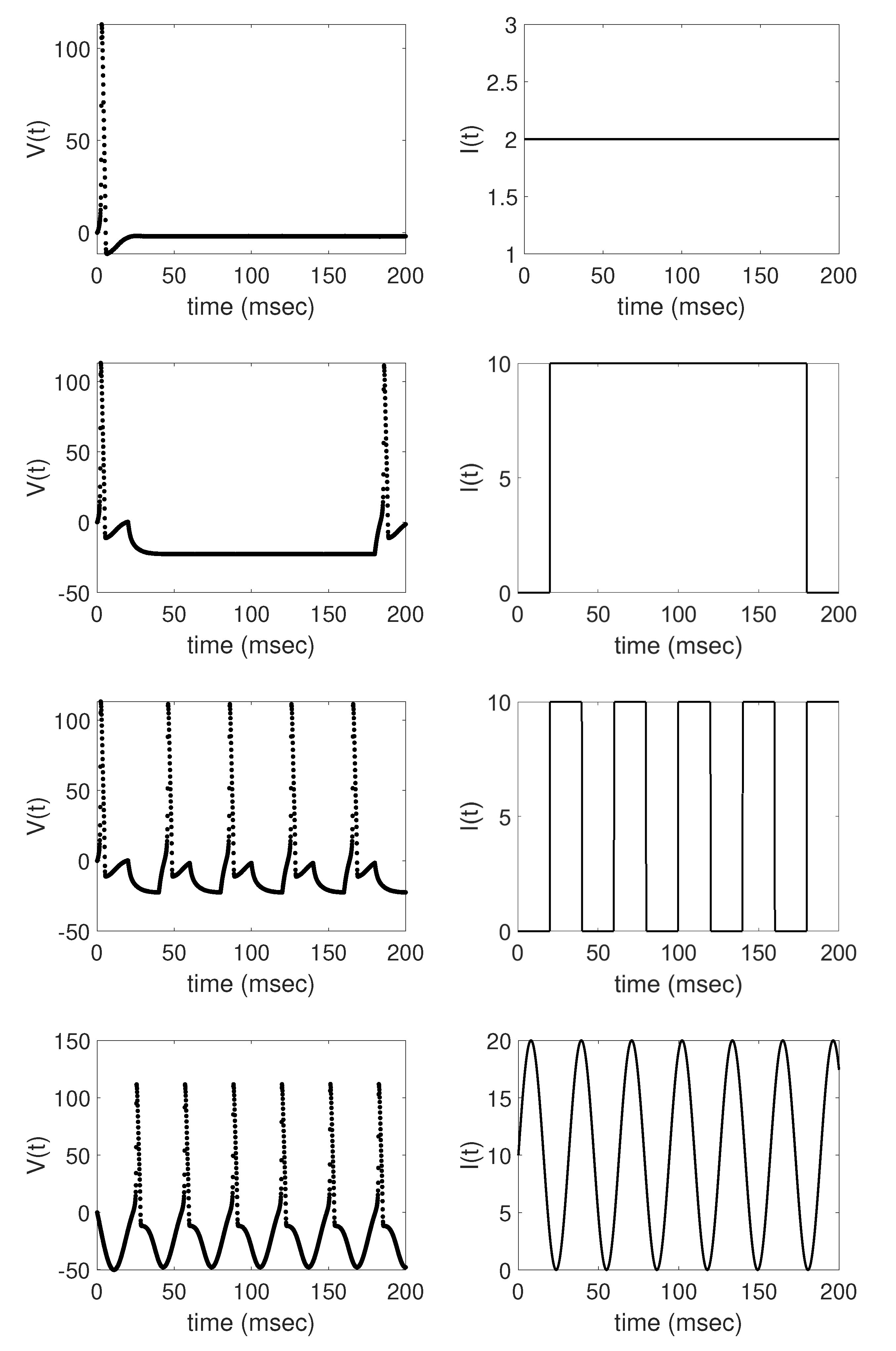
In this work, we analyze the problem of estimating the time-varying applied current in the Hodgkin-Huxley model using synthetic voltage data generated by applying four different deterministic functions as the applied current—a constant current, a step function with one long pulse, a step function with multiple shorter pulses, and a sinusoidal function—each resulting in different model dynamics. We establish baseline results, demonstrating that the augmented EnKF with parameter tracking is able to estimate well the applied current and unobserved Hodgkin-Huxley model components in each of these four cases. We then further test the efficiency of the algorithm by performing numerical experiments to analyze the effects of changing the standard deviation of the drift term in the parameter tracking as well as the frequency of data available on the resulting applied current parameter estimates, including the corresponding uncertainty.

The paper is organized as follows. Section 2 gives a brief review of the Hodgkin-Huxley model, summarizing the relevant equations. Section 3 reviews the parameter estimation inverse problem and outlines the ensemble Kalman filtering algorithm, with specific focus on time-varying parameter estimation using the EnKF with parameter tracking. Section 4 describes the numerical results, including the generation of synthetic data and the numerical experiments relating to estimating the time-varying applied current parameter. Section 5 features a discussion of the results and future work, while Section 6 gives a brief summary and conclusions of this work. Additional numerical experiments are included in Appendix A.

2. Review of the Hodgkin-Huxley Model Equations

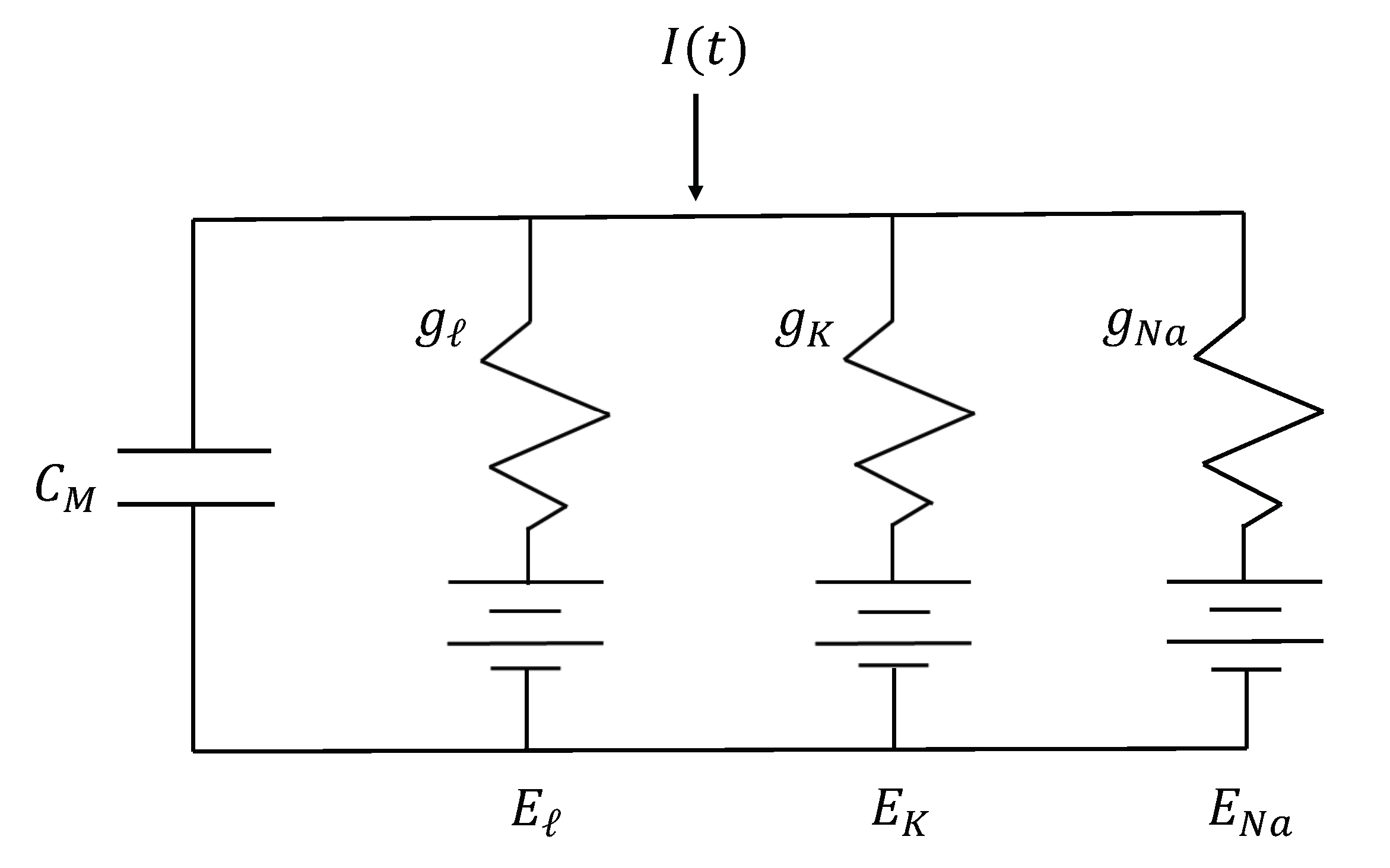
The Hodgkin-Huxley model provided the first quantitative description of electrical excitability in nerve cells [24], involving detailed mathematical equations to describe the voltage-dependent and time-dependent properties of the sodium and potassium conductances [1]. Each piece of the circuit shown in Figure 1 corresponds to a different electrophysiological component of the model. Capacitors represent the charge storage capacity of each gating variable; resistors represent the sodium, potassium, and leakage ion channels in the neuron; and batteries represent the electrochemical potentials that each gating variable has to let ions in and out of the charged cell.

From this analogy, the Hodgkin-Huxley equation modeling total membrane current is given by

$$I=C_M\frac{dV}{dt}+I_{ion}$$

(1)

where $I=I\left(t\right)$ is the total membrane current in the axon (with a positive inward current), $C_M$ is the membrane capacity (assumed to be constant), and $V=V\left(t\right)$ is the displacement of the membrane potential from its resting value (assumed to have a negative depolarization).

Table 1. Components of the Hodgkin-Huxley model (1).

Component	Description	Units
I	Total membrane current	mA/cm2
$C_M$	Membrane capacity	$\mathsf{\mu }$F/cm2
V	Voltage	mV
$I_{ion}$	Ionic current density	mA/cm2
t	Time	msec

lists each model component, along with its corresponding units. For simplicity of terminology, we will refer interchangeably to $V\left(t\right)$ as the voltage within this paper. Note that the voltage V is related to the membrane potential E via the relationship $V=E-E_r$, where $E_r$ denotes the absolute value of the resting potential [1].

The ionic current density $I_{ion}$ is represented as the sum of the three currents

$$I_{ion}=I_{Na}+I_K+I_{\ell }$$

(2)

where $I_{Na}$, $I_K$, and $I_{\ell }$ model the currents relating to the sodium, potassium, and leakage channels occurring in the neuron, respectively. The form of the current for each ion channel follows from Ohm’s law, where

$$I_i=g_i(t,V)(V-V_i)$$

(3)

for $i=Na,K,\ell$. Here $g_i(t,V)$ represents the gate for each channel generally as a function of time and voltage, and $V-V_i$ represents the difference between the overall voltage V of the system and the channel-specific voltages $V_i$. We describe each of the three ionic currents in more detail as follows.

Sodium current. The sodium current is given by

$$I_{Na}=g_{Na}(t,V)(V-V_{Na})$$

(4)

where the sodium gate

$$g_{Na}(t,V)=m^{3}h{\overline{g}}_{Na}$$

(5)

is impacted by depolarization, which causes an increase in sodium conductance [1]. Here ${\overline{g}}_{Na}$ is a constant (conductance/cm²), $m=m\left(t\right)$ is the proportion of active sodium gates open (dimensionless variable which varies over time between 0 and 1), and $h=h\left(t\right)$ is the proportion of inactive gates open (similarly dimensionless, varying between 0 and 1). The sodium voltage is given by $V_{Na}=E_{Na}-E_r$, where $E_{Na}$ is an equilibrium potential for sodium.

Table 2. Constant parameter values used in the Hodgkin-Huxley model. Note that m.mho stands for 1/ohm (the reverse of ohm) or amp/volts. It is the unit Siemen and represents the derived unit of electrical conductance.

Parameter	Description	Value	Units
$C_M$	Membrane capacity	1.0	$\mathsf{\mu }$F/cm2
$V_{Na}$	Sodium voltage	−115	mV
$V_K$	Potassium voltage	12	mV
$V_{\ell }$	Leakage voltage	−10.613	mV
${\overline{g}}_{Na}$	Sodium gate constant	120	m.mho/cm2
${\overline{g}}_K$	Potassium gate constant	36	m.mho/cm2
${\overline{g}}_{\ell }$	Leakage gate constant	0.3	m.mho/cm2

lists the constant values of $V_{Na}$ and ${\overline{g}}_{Na}$.

The dynamics of the sodium gating variables $m\left(t\right)$ and $h\left(t\right)$ are governed by the following differential equations:

$$\begin{array}{ccc}\hfill \frac{dm}{dt}& =& {\alpha }_m\left(V\right)(1-m)-{\beta }_m\left(V\right)m\hfill \end{array}$$

(6)

$$\begin{array}{ccc}\hfill \frac{dh}{dt}& =& {\alpha }_h\left(V\right)(1-h)-{\beta }_h\left(V\right)h\hfill \end{array}$$

(7)

where the voltage-dependent rate constants (msec⁻¹) ${\alpha }_m$ and ${\alpha }_h$ represent the rate of flow of ions into the cell and ${\beta }_m$ and ${\beta }_h$ represent the flow out. The rate constants are modeled using the following equations, derived from Hodgkin and Huxley’s experimental results [1]:

$$\begin{array}{ccc}\hfill {\alpha }_m\left(V\right)& =& \frac{0.1(V+25)}{exp\left(\frac{V+25}{10}\right)-1}\hfill \end{array}$$

(8)

$$\begin{array}{ccc}\hfill {\alpha }_h\left(V\right)& =& 0.07exp\left(\frac{V}{20}\right)\hfill \end{array}$$

(9)

$$\begin{array}{ccc}\hfill {\beta }_m\left(V\right)& =& 4exp\left(\frac{V}{18}\right)\hfill \end{array}$$

(10)

$$\begin{array}{ccc}\hfill {\beta }_h\left(V\right)& =& \frac{1}{exp\left(\frac{V+30}{10}\right)+1}\hfill \end{array}$$

(11)

Note that setting ${\alpha }_m$ to its limit value of 1 at $V=-25$ mV avoids the discontinuity at that point.

Potassium current. The potassium current is given by

$$I_K=g_K(t,V)(V-V_K)$$

(12)

with potassium gate equation

$$g_K(t,V)={\overline{g}}_K{n}^4.$$

(13)

Here ${\overline{g}}_K$ is a constant (conductance/cm²) and $n=n\left(t\right)$ is the proportion of potassium gates open (dimensionless, varying between 0 and 1). The potassium voltage is given by $V_K=E_K-E_r$, where $E_K$ is an equilibrium potential for potassium, sensitive to the overall outside concentration of charged ions [25]. Table 2 lists the constant values of $V_K$ and ${\overline{g}}_K$.

The dynamics of the gating variable $n\left(t\right)$ are similarly modeled using the differential equation

$$\frac{dn}{dt}={\alpha }_n\left(V\right)(1-n)-{\beta }_n\left(V\right)n$$

(14)

where the rate constants

$$\begin{array}{c}\hfill {\alpha }_n\left(V\right)=\frac{0.01(V+10)}{exp\left(\frac{V+10}{10}\right)-1}\end{array}$$

(15)

$$\begin{array}{c}\hfill {\beta }_n\left(V\right)=0.125exp\left(\frac{V}{80}\right)\end{array}$$

(16)

were also derived using experimental data [1]. Note the discontinuity in ${\alpha }_n$ when $V=-10$ mV can be avoided by setting it equal to its limit value of 0.1 at that point.

Leakage current. The leakage current is a small combined current, accounting mostly for chloride but also other ions. The leakage current is given by

$$I_{\ell }={\overline{g}}_{\ell }(V-V_{\ell })$$

(17)

with constant conductance ${\overline{g}}_{\ell }$ and leakage voltage $V_{\ell }=E_{\ell }-E_r$. Here $E_{\ell }$ is the potential at which the leak current is zero. The leakage voltage $V_{\ell }$ is needed for any calculation for threshold, but it is unlikely to give any information about the nature of charged particles [25]. Table 2 lists the constant values of $V_{\ell }$ and ${\overline{g}}_{\ell }$.

Model summary. In summary, the Hodgkin-Huxley model comprises the total membrane current Equation (1), which depends on time, voltage, and the solutions to the transfer Equations (6), (7) and (14). Note that when a constant voltage is applied, $\frac{dV}{dt}=0$ and (1) simplifies to $I=I_{ion}$. In this case, Equations (6), (7) and (14) can be solved independently to compute the total ionic current.

However, when voltage changes with time due to an applied current, $\frac{dV}{dt}\ne 0$ and all four equations must be solved simultaneously. The complete system of coupled ordinary differential equations is given by

$$\begin{array}{ccc}\hfill \frac{dV}{dt}& =& \frac{1}{C_M}(I-I_{ion})\hfill \end{array}$$

(18)

$$\begin{array}{ccc}\hfill \frac{dn}{dt}& =& {\alpha }_n\left(V\right)(1-n)-{\beta }_n\left(V\right)n\hfill \end{array}$$

(19)

$$\begin{array}{ccc}\hfill \frac{dm}{dt}& =& {\alpha }_m\left(V\right)(1-m)-{\beta }_m\left(V\right)m\hfill \end{array}$$

(20)

$$\begin{array}{ccc}\hfill \frac{dh}{dt}& =& {\alpha }_h\left(V\right)(1-h)-{\beta }_h\left(V\right)h\hfill \end{array}$$

(21)

Note that in this case, the applied current $I=I\left(t\right)$ in (18) drives the system dynamics. We explore how different choices of deterministic, time-varying functions for $I\left(t\right)$ affect the dynamics of the system in the numerical results.

3. Parameter Estimation and the Ensemble Kalman Filter

Given measurements of voltage, our aim is to estimate the time-varying applied current $I\left(t\right)$ that best fits the available data. This is a parameter estimation inverse problem, where the parameter of interest is a time-varying deterministic function with assumed unknown dynamics. More specifically, we assume here that we cannot directly measure the time-varying applied current and that we do not have equations available to explain its dynamics.

The set-up for this inverse problem is similar to the standard set-up for estimating parameters in initial value problems of the form

$$\frac{dx}{dt}=f(t,x,\theta ),x\left(0\right)=x_0$$

(22)

where $x=x\left(t\right)$ denotes the model states and $\theta$ denotes the model parameters [19]. Given some discrete, noisy system measurements

$$y_j=G(x\left(t_j\right),\theta )+w_j,0<t_1<\cdots <t_T$$

(23)

the inverse problem is to estimate the model states $x\left(t\right)$ and parameters $\theta$. Most classical approaches addressing this problem tend to focus on the case when the parameters are constants, i.e., when $\frac{d\theta }{dt}=0$. In this case, however, $\theta =\theta \left(t\right)$ and $\frac{d\theta }{dt}$ is some unknown function.

To estimate the time-varying applied current in this work, we use a version of the ensemble Kalman filter (EnKF) with parameter tracking [16,19]. The EnKF is an extension of the classical Kalman filter adapted to work with models that are not necessarily linear or Gaussian [12,13]. As a Bayesian statistical algorithm, the EnKF treats all unknowns as random variables with corresponding probability distributions. The filter uses a random sample to represent the current probability distribution of states and parameters, then utilizes ensemble statistics along with model predictions and observed data to update the sample at each discrete time point.

While the original EnKF was implemented for state estimation, the augmented EnKF allows for simultaneous state and parameter estimation [26]. The steps of the augmented EnKF are summarized as follows. At time j, the sample

$$S_{j\mid j}=\left\{(x_{j\mid j}^1,{\theta }_{j\mid j}^1),(x_{j\mid j}^2,{\theta }_{j\mid j}^2),\cdots ,(x_{j\mid j}^N,{\theta }_{j\mid j}^N)\right\}$$

(24)

gives a discrete representation of the probability distribution, which is then updated using a two-step process to time $j+1$. In the first step (the prediction step), we solve the system (22) to predict the state values at time $j+1$. In this work, (22) is the Hodgkin-Huxley model given in (18)–(21). The state prediction ensemble is computed using the equation

$$x_{j+1\mid j}^p=F(x_{j\mid j}^p,{\theta }_j^p)+v_{j+1}^p,p=1,2,\cdots ,N$$

(25)

where F is the solution to (22) at time $j+1$ and $v_{j+1}^p\sim \mathcal{N}(0,\mathrm{C})$ represents error in the model prediction. The predicted states $x_{j+1\mid j}^p$ and current parameter values ${\theta }_j^p$ are then placed in the augmented vectors

$$z_{j+1\mid j}^p=\left[\begin{array}{c}{x}_{j+1\mid j}^p\\ {\theta }_j^p\end{array}\right],p=1,2,\cdots ,N$$

(26)

which are used to compute ensemble statistics. The prediction ensemble mean is computed using the formula

$${\overline{z}}_{j+1\mid j}=\frac{1}{N}\sum _{p=1}^N{z}_{j+1\mid j}^p$$

(27)

and the prior covariance matrix by

$${\Gamma }_{j+1\mid j}=\frac{1}{N-1}\sum _{p=1}^N(z_{j+1\mid j}^p-{\overline{z}}_{j+1\mid j}){(z_{j+1\mid j}^p-{\overline{z}}_{j+1\mid j})}^T.$$

(28)

Note that while the parameters ${\theta }_j^p$ are not updated in the prediction step, their cross-correlation information with the predicted states is embedded in the prior covariance matrix and is used in the next step to update the posterior sample.

In the second step (the observation update), the predicted values are compared with the observed data $y_{j+1}$ at time $j+1$. The observation ensemble

$$y_{j+1}^p=y_{j+1}+w_{j+1}^p,p=1,2,\cdots ,N$$

(29)

where $w_{j+1}^p\sim \mathcal{N}(0,\mathrm{D})$ represents the observation error, is compared to the observation model predictions

$${\widehat{y}}_{j+1}^p=G(x_{j+1\mid j}^p,{\theta }_j^p),p=1,2,\cdots ,N$$

(30)

computed using the observation model G as in (23). In this work, G is a linear observation function measuring only the voltage in the Hodgkin-Huxley system. The combined posterior ensemble is then given by

$$z_{j+1\mid j+1}^p=z_{j+1|j}^p+K_{j+1}(y_{j+1}^p-{\widehat{y}}_{j+1}^p)$$

(31)

for each $p=1,2,\cdots ,N$. The Kalman gain matrix $K_{j+1}$ incorporates the cross-covariance of state and model predications, the forecast error covariance, and the observation noise covariance. For additional implementation details, see [19,27].

Parameter tracking. In the above formulation of the augmented EnKF, $\theta$ is assumed to be constant and is evolved artificially with time in order to obtain an estimate. When $\theta$ is time-varying, as in the case we are considering, the augmented EnKF as presented requires additional modification. If $\theta =\theta \left(t\right)$ changes more slowly than the dynamics of the system, it is possible to track the changes in $\theta \left(t\right)$ by incorporating a random walk in the prediction step. To implement this, a new random variable $\xi$ is introduced and added to current estimate of $\theta$ at each prediction step, allowing the previously fixed parameters to take a random walk of the form

$${\theta }_{j+1\mid j}^p={\theta }_{j\mid j}^p+{\xi }_j^p,{\xi }_j^p\sim \mathcal{N}(0,{\sigma }_{\xi }^2)$$

(32)

for each $p=1,2,\cdots ,N$. Parameter tracking of this type has been used in various data assimilation problems; see, e.g., [14,15,16,28]. Here we note that the choice of the standard deviation ${\sigma }_{\xi }$ in the drift term of the random walk is important in the accuracy and uncertainty of the resulting parameter estimate. We will explore this further in the numerical experiments.

4. Numerical Experiments

In this section we describe the numerical experiments performed using the augmented EnKF with parameter tracking to estimate the time-varying applied current in the Hodgkin-Huxley model. All experiments were performed using the MATLAB^® programming language. In particular, we used the built-in solver ode15s to numerically solve (18)–(21) due to the potential stiffness of the system when applying different time-varying currents. We first describe how synthetic data was generated using four deterministic applied currents. We then provide the numerical results obtained using parameter tracking to estimate the applied current in each case. We further explore the efficiency of the algorithm by analyzing the effects of changing the standard deviation of the parameter drift in (32) as well as the amount of time series voltage data available. Additional numerical experiments, including a comparison between estimating a sinusoidal current and constant current of higher amplitude, are included in Appendix A.

4.1. Synthetic Data Generation

To generate synthetic data, four different deterministic functions for the applied current $I\left(t\right)$ were run through the Hodgkin-Huxley Equations (18)–(21). The applied currents considered were:

(a)

a constant current, where

$$I\left(t\right)=2\mathrm{mA}/{\mathrm{cm}}^2$$

(33)

(b)

a step function with one long pulse, such that

$$I\left(t\right)=\left\{\begin{array}{cc}0\mathrm{mA}/{\mathrm{cm}}^2,\hfill & t\in [0,20)\hfill \\ 10\mathrm{mA}/{\mathrm{cm}}^2,\hfill & t\in [20,160)\hfill \\ 0\mathrm{mA}/{\mathrm{cm}}^2,\hfill & t\in [160,200]\hfill \end{array}\right.$$

(34)

(c)

a “pulsing” step function with multiple short pulses, such that

$$I\left(t\right)=\left\{\begin{array}{cc}0\mathrm{mA}/{\mathrm{cm}}^2,\hfill & t\in [20q,20+20q),\hfill \\ \hfill & q=0,2,4,6,8\hfill \\ 10\mathrm{mA}/{\mathrm{cm}}^2,\hfill & t\in [20q,20+20q),\hfill \\ \hfill & q=1,3,5,7,9\hfill \end{array}\right.$$

(35)

(d)

a sinusoidal function, where

$$I\left(t\right)=10sin(0.2t)+10\mathrm{mA}/{\mathrm{cm}}^2.$$

(36)

For each data set, measurements of voltage $V\left(t\right)$ were taken at 2001 equidistant time instances over the interval $[0,200]$ and corrupted by Gaussian noise with zero mean and standard deviation 0.05. Figure 2 shows each data sets along with the corresponding applied current. Note that the gating variables $n\left(t\right)$, $m\left(t\right)$, and $h\left(t\right)$ are unobserved states.

4.2. Estimating Time-Varying Applied Current via Parameter Tracking

We first establish baseline results for each of the four data sets described in Section 4.1 by applying the augmented EnKF with parameter tracking to estimate the time-varying applied current and Hodgkin-Huxley model states. We then perform numerical experiments to analyze the effects of the standard deviation of the parameter drift term in (32) and the frequency of time series voltage data available on the resulting applied current parameter estimates.

Baseline results. To establish baseline results for parameter tracking in each of the four data sets described in Section 4.1, we employ the augmented EnKF with parameter tracking using $N=100$ ensemble members with the standard deviation of the parameter random walk in (32) set to ${\sigma }_{\xi }=1$. Initial ensembles for the model states $x\left(t\right)=\left[V\right(t);n(t);m(t);h(t\left)\right]$ and applied current parameter $\theta \left(t\right)=I\left(t\right)$ were drawn from uniform prior distributions, with $V_{0\mid 0}^p\sim \mathcal{U}(-100,0)$; $n_{0\mid 0}^p,m_{0\mid 0}^p,h_{0\mid 0}^p\sim \mathcal{U}(0,1)$; and $I_{0\mid 0}^p\sim \mathcal{U}(0,4)$ for each $p=1,2,\cdots ,N$. The results in Figure 3, Figure 4, Figure 5 and Figure 6 show the parameter tracking estimates of $I\left(t\right)$, along with the time series estimates of the Hodgkin-Huxley model states, for each of the four cases. Note that in each case, the filter mean is able to track the underlying true applied current, along with the unmeasurable system states, with uncertainty bounds represented by the $\pm 2$ estimated standard deviation curves.

Standard deviation of parameter drift. As noted in Section 3, a carefully chosen standard deviation ${\sigma }_{\xi }$ for the random walk in (32) is crucial in maintaining the accuracy of the time-varying parameter estimate and avoiding filter divergence; see, e.g., [21,22,23,27] and references therein. To demonstrate the sensitivity of the parameter tracking algorithm to this choice, we tested the effects of changing ${\sigma }_{\xi }$ by letting ${\sigma }_{\xi }=10$, 2, 1, 0.5, 0.25, and 0.1 in estimating the applied current, compared with ${\sigma }_{\xi }=1$ used in the baseline results above. For sake of demonstration, we focused on the data generated using the sinusoidal current defined in (36); similar results hold in the other cases.

The results in Figure 7 show that when ${\sigma }_{\xi }=10$, although the EnKF mean estimate was able to well track the true solution, the estimated $\pm 2$ standard deviation curves around the mean are very large around the mean, reflecting a lack of confidence in the estimate. On the other hand, when ${\sigma }_{\xi }=0.1$, the filter is unable to well track the true parameter and eventually diverges. In this case, while the filter is unable to track the true parameter, the estimated $\pm 2$ standard deviation curves are very tight around the mean, implying a high confidence in an incorrect estimate. For this example, the choice of ${\sigma }_{\xi }=0.5$ in the parameter random walk visually captures the true underlying parameter the best out of the values considered, as it keeps the EnKF estimated mean closely with a small standard deviation around the mean.

Frequency of data available. In addition to the choice of ${\sigma }_{\xi }$, the frequency of time series data available also has a significant effect on the resulting parameter tracking estimates. To analyze this on the problem at hand, we subsampled the available voltage data corresponding to the pulsing step current (35) and sinusoidal current (36) every 10, 20, and 50 time points, resulting in data sets containing 201, 101, and 41 equidistant voltage observations over the time interval $[0,200]$. This means that data was considered in the observation step in the EnKF every first, second, or fifth millisecond (as compared to every 0.1 msec using the full data). Note that the filter still performed the prediction step every 0.1 msec as before, but the observation step was only preformed if data was available at that time point.

The results in Figure 8 and Figure 9 show that as data becomes more and more sparse, the parameter tracking estimate of the applied current parameter loses more and more characteristics of the underlying deterministic function. In particular, in Figure 8, as less data is available, the parameter tracking estimate of the pulsing step function begins lagging in estimating the steps and is unable to well maintain the shape. Similar results are seen in Figure 9 for the sinusoidal function, where the parameter tracking estimate loses its periodicity as less data becomes available. In both figures, it is clear that the sparser the data set, the more challenging it becomes for the filter to track the true underlying applied current function.

5. Discussion

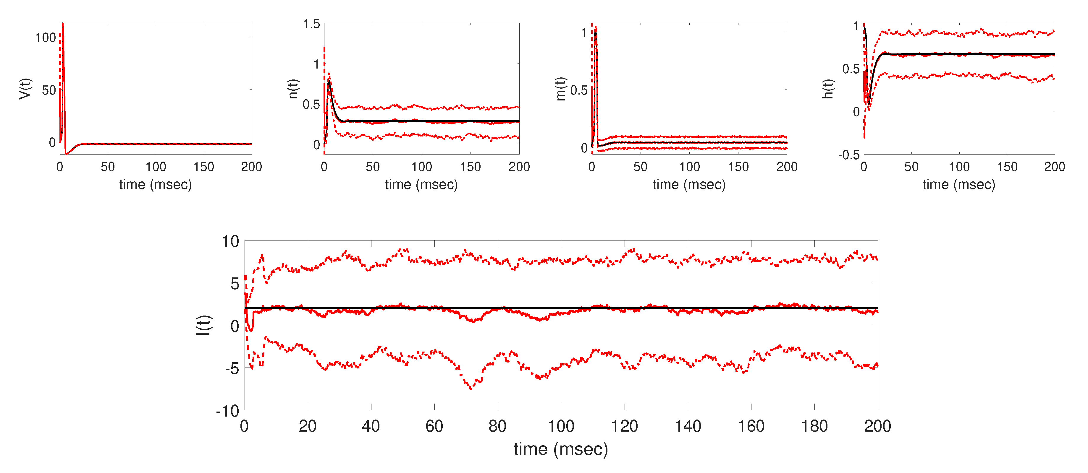
The aim of this work was to utilize the EnKF with parameter tracking in estimating the time-varying applied current parameter in the Hodgkin-Huxley model. In particular, the parameter tracking algorithm was analyzed in estimating four different deterministic applied currents using synthetically-generated voltage data. We first verified that the algorithm was able to successfully track the underlying applied current, along with the unobserved model states, for each of the four test cases. In addition to tracking the applied current $I\left(t\right)$, baseline results show that the filter is able to accurately estimate the unobserved states $n\left(t\right)$, $m\left(t\right)$, and $h\left(t\right)$ from the generated voltage data. Further numerical experiments were conducted to analyze how the parameter tracking estimates of the applied current parameter are affected under different implementation conditions, namely, when changing the standard deviation of the parameter drift term in (32) and when the algorithm is provided increasingly less voltage data.

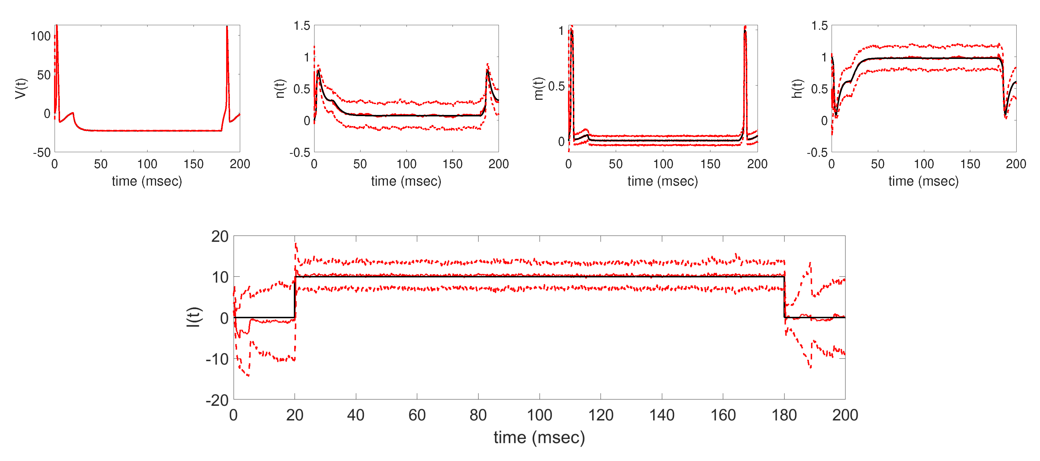
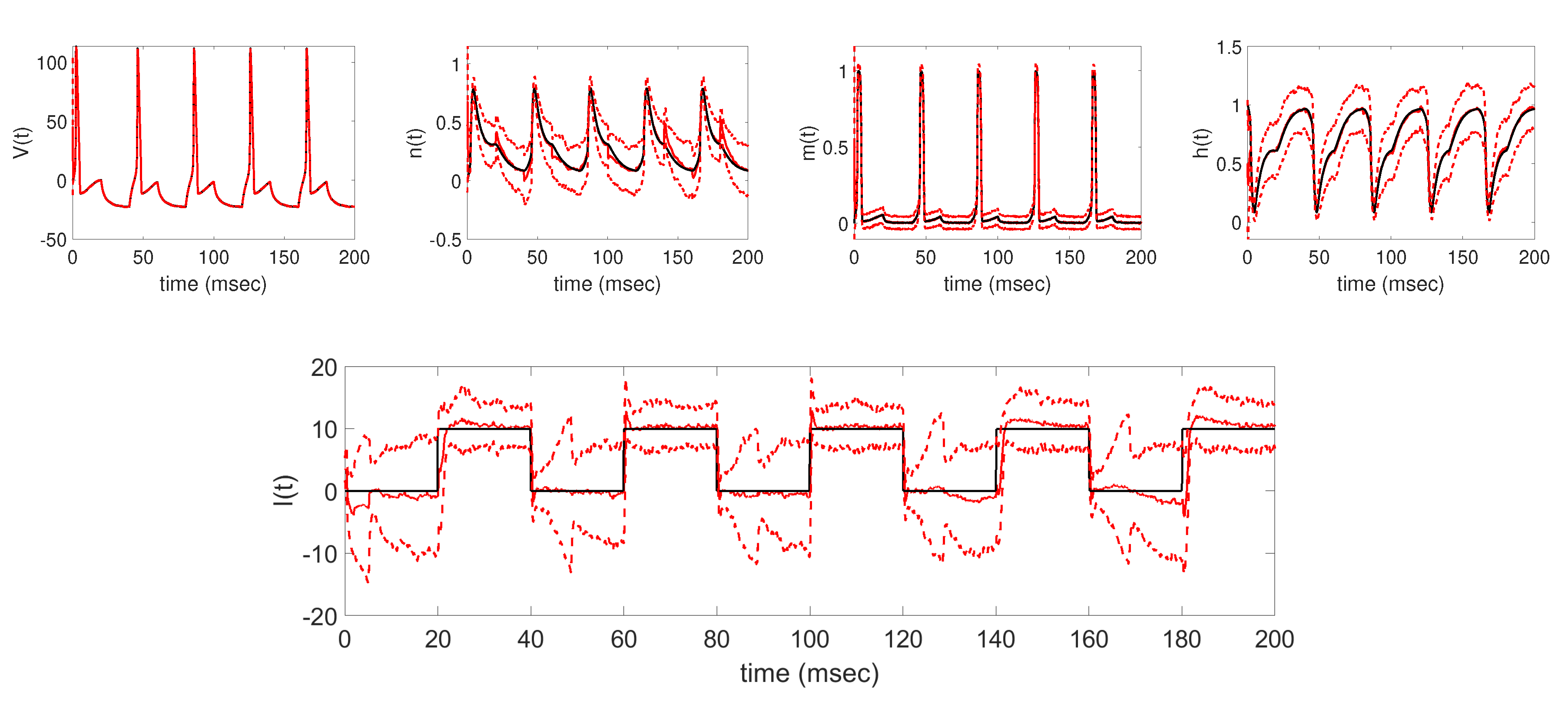
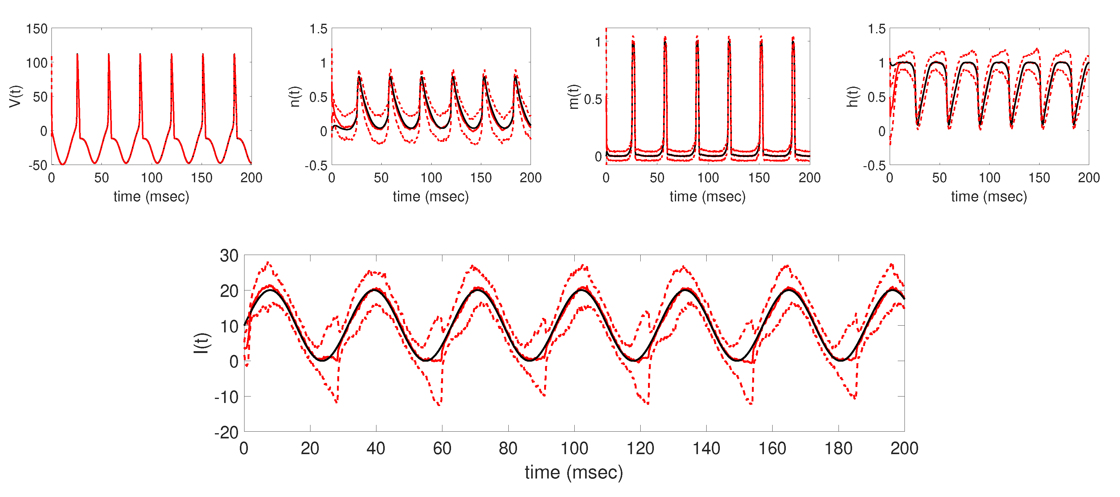
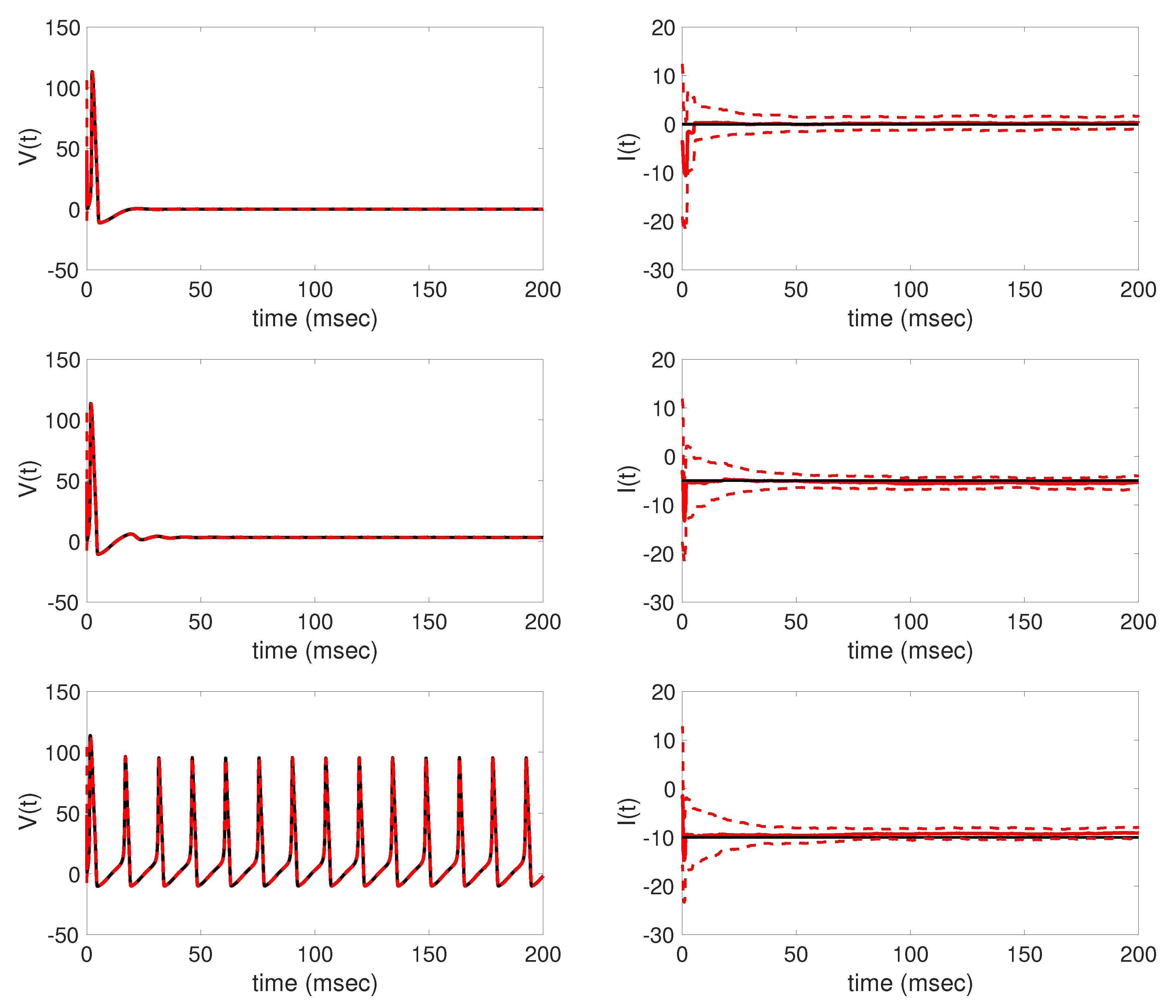
Overall, using the augmented EnKF with parameter tracking as described in Section 3, we were able to well track the underlying applied current functions in each of the four cases considered, establishing the baseline results shown in Figure 3, Figure 4, Figure 5 and Figure 6. In each case, the EnKF mean well approximates the true underlying applied current, in cases where the current is constant, a single pulse, multiple pulses, and a sinusoidal function, as well as the corresponding model states. Uncertainty bounds around the EnKF estimates, as reflected in the estimated $\pm 2$ standard deviation curves around the mean, in each case well contain the true applied current and associated model states, with less uncertainty around the measured voltage than the unobserved gating variables. From the baseline results, we were able to further explore the effects of two important aspects of the parameter tracking implementation: the choice of the standard deviation of the parameter drift term in (32), and the availability of time series voltage data.

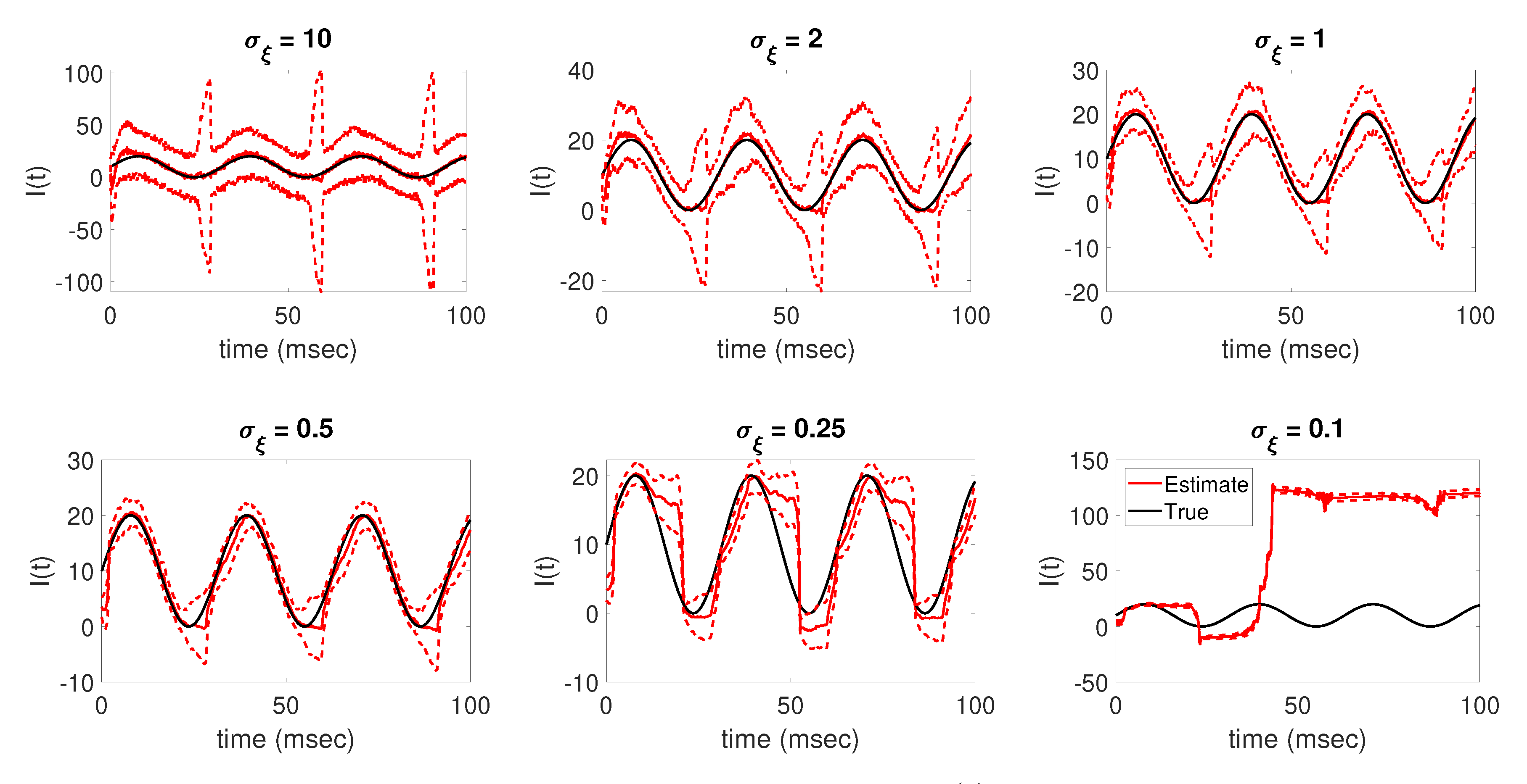
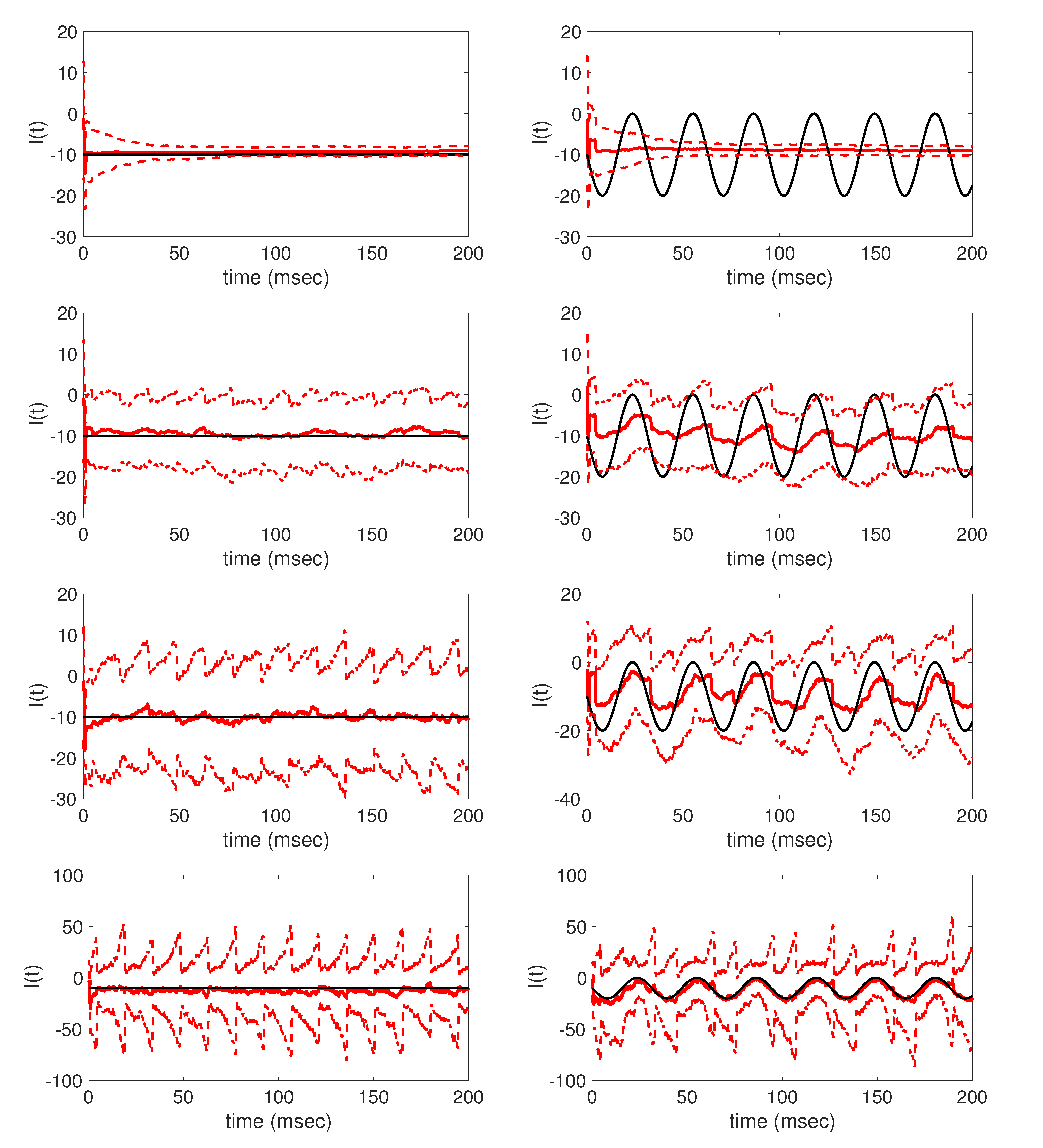
Numerical experiments showed that using different values for ${\sigma }_{\xi }$ results in drastically different levels of accuracy and confidence in the parameter tracking estimates for the applied current. As shown in Figure 7, when using ${\sigma }_{\xi }=10$ for the parameter drift standard deviation, the resulting EnKF mean estimate is able to well track the true current; however, the resulting confidence in the estimate is low, as reflected in the wide range between the estimated $\pm 2$ standard deviation curves. Oppositely, when using ${\sigma }_{\xi }=0.1$, the parameter tracking estimate diverges from the true solution, returning an estimate of the applied current parameter that is significantly inaccurate despite having high confidence in the estimate, as reflected in the tight uncertainty bounds. The results in Figure 7 suggest that, for the data considered, ${\sigma }_{\xi }=0.5$ is the best choice for the parameter drift standard deviation out of the values tested for this problem, with the corresponding applied current estimate accurately tracking the true solution with less uncertainty reflected in the resulting $\pm 2$ standard deviation curves around the EnKF mean than for larger ${\sigma }_{\xi }$ values.

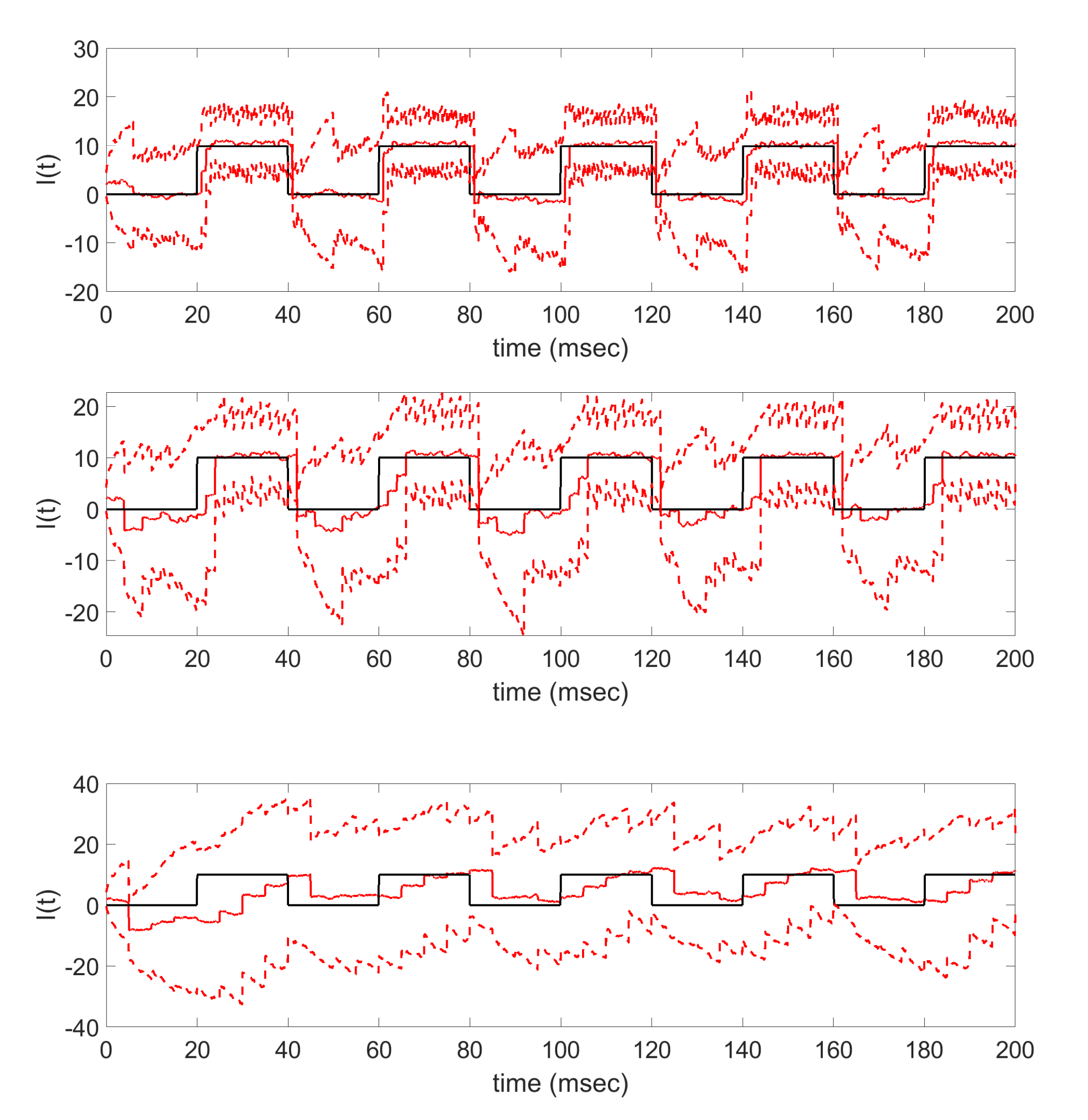
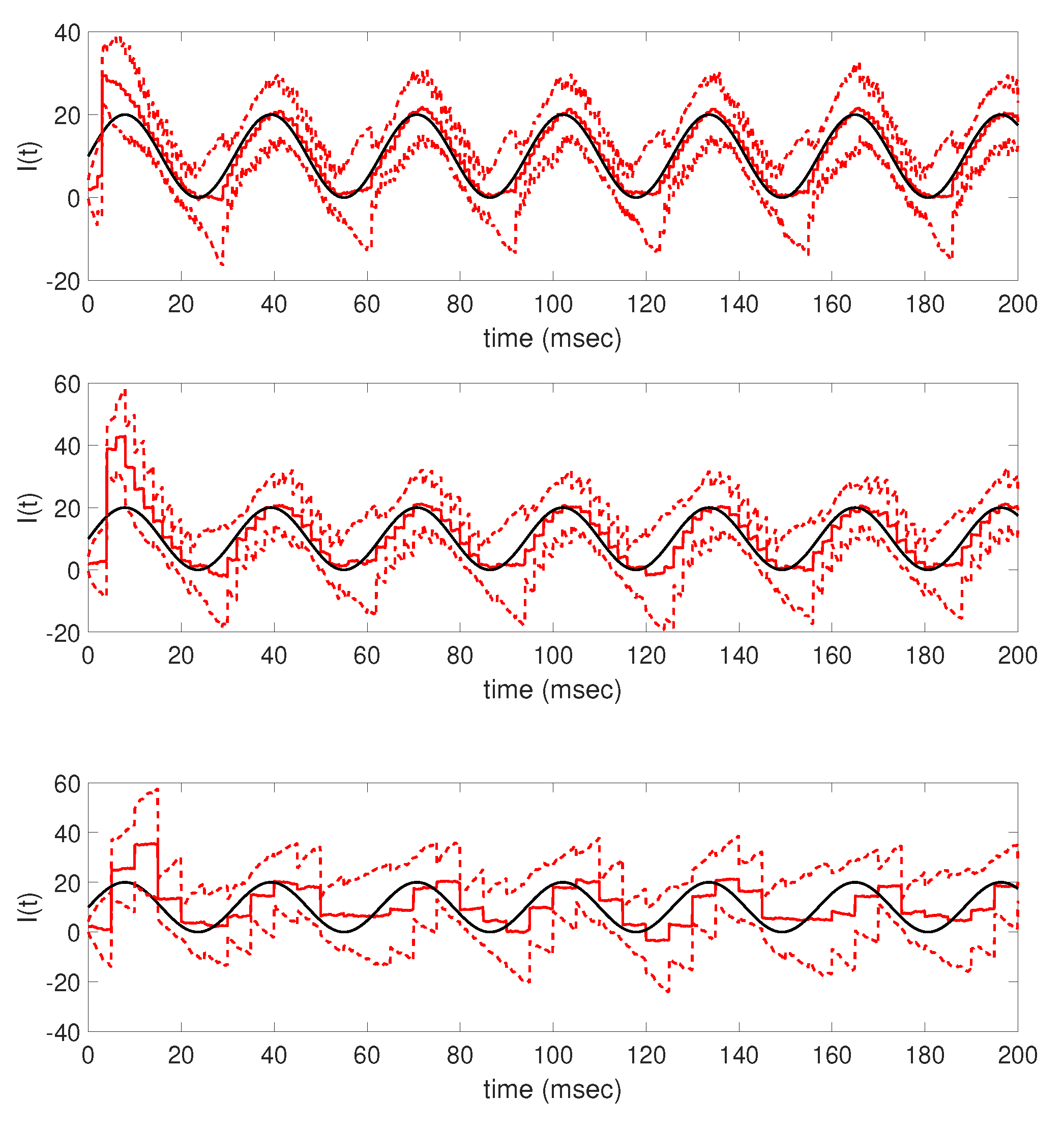
Further numerical tests demonstrate how the accuracy of the parameter tracking estimate is affected when the frequency of available time series voltage data is decreased, resulting in fewer data points being used as updating information in the filter. The results in Figure 8 and Figure 9 show that as less data is made available via subsampling, the parameter tracking algorithm has increasing difficulty in estimating the true underlying applied current function, losing structural features such as the step onset of the pulsing step current and the periodicity of the sinusoidal current. In this work, the generated data was subsampled at equidistance time points, resulting in less frequent but equispaced voltage observations; future work may consider the effects of measurement times as well as frequency on the resulting time-varying applied current estimates in order to further explore the importance of data availability in obtaining accurate time-varying parameter estimates.

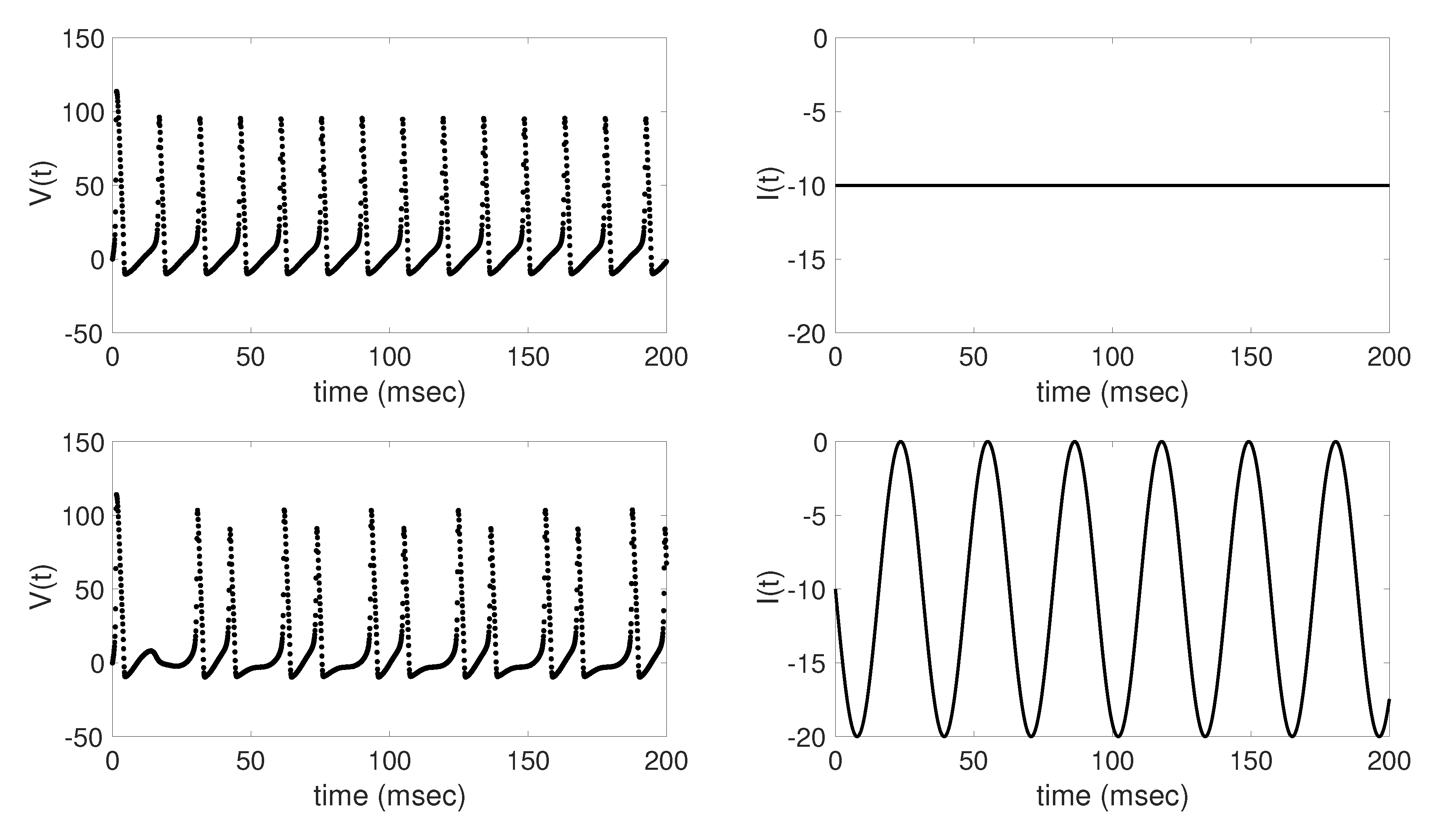
Additional numerical experiments contained in Appendix A demonstrate the capability of the EnKF with parameter tracking in estimating constant currents of increasing amplitude, as well as the capability of the algorithm in distinguishing a higher-amplitude constant current from a time-varying sinusoidal current with similar multiple-spiking voltage data. The results in Figure A1 show that the parameter tracking algorithm can well capture the behavior of the applied current for increasing magnitude using a relatively small choice of parameter drift standard deviation ${\sigma }_{\xi }$. However, the results in Figure A3 further demonstrate the importance of choosing an appropriate value for ${\sigma }_{\xi }$ in the parameter tracking algorithm, as this choice also has a significant impact on the filter’s ability to distinguish between a constant and time-varying current.

While the focus of this work is on estimating different deterministic forms of the time-varying applied current parameter, in future work we aim to estimate stochastic forms of the current, as well as estimating applied currents relating to networks of neurons. In addition to the applied current, we are also interested in applying parameter tracking methodology to estimate the $\alpha \left(V\right)$ and $\beta \left(V\right)$ rate functions as additional unknown parameters that vary with voltage, which would be particularly useful in applications of the Hodgkin-Huxley model where these rate functions do not necessarily share the same parameterized forms as in (8)–(11) and (15)–(16).

Future work also includes comparing our results for the Hodgkin-Huxley model with results using other single neuron models, such as the FitzHugh-Nagumo and Hindmarsh-Rose models [29,30,31]. We further aim to apply our results to biomedical applications utilizing Hodgkin-Huxley dynamics to model various neurodegenerative diseases affecting the function of neurons and ionic channels, such as Alzheimer’s disease and amyotrophic lateral sclerosis [32,33,34]. The methodology used in this work can be employed in developing patient-specific models for personalized medicine applications, with the potential of identifying possible differences in time-varying input stimuli between healthy and disease states.

6. Summary and Conclusions

The classical Hodgkin-Huxley model is widely employed in simulating the electrophysiological dynamics of a single neuron. While voltage measurements are commonly obtainable in experimental settings, information regarding the synaptic input stimuli may be unavailable or difficult to measure. In this work, we consider the inverse problem of estimating the applied current given voltage data. In particular, we utilize ensemble Kalman filtering with parameter tracking to estimate the Hodgkin-Huxley model states and time-varying applied current parameter of different deterministic functional forms given synthetically-generated measurements of voltage. Our results demonstrate the importance of choosing an appropriate parameter drift standard deviation in the parameter tracking algorithm, as well as the importance of having frequent time series voltage measurements, in estimating the underlying time-varying applied current well.

References

1. Hodgkin, A.L.; Huxley, A.F. A quantitative description of membrane current and its application to conduction and excitation in nerve. J. Physiol. 1952, 117, 500–544. [Google Scholar] [CrossRef] [PubMed]
2. Ermentrout, G.B.; Terman, D.H. Mathematical Foundations of Neuroscience; Interdisciplinary Applied Mathematics; Springer: New York, NY, USA, 2010; Volume 35. [Google Scholar] [CrossRef] [Green Version]
3. Nelson, M.E. Electrophysiological Models. In Databasing the Brain: From Data to Knowledge; Wiley: Hoboken, NJ, USA, 2004. [Google Scholar]
4. Lynch, E.P.; Houghton, C.J. Parameter estimation of neuron models using in-vitro and in-vivo electrophysiological data. Front. Neuroinform. 2015, 9, 1–15. [Google Scholar] [CrossRef] [PubMed] [Green Version]
5. Wei, Y.; Ullah, G.; Parekh, R.; Ziburkus, J.; Schiff, S.J. Kalman filter tracking of intracellular neuronal voltage and current. In Proceedings of the 50th IEEE Conference on Decision and Control and European Control Conference, Orlando, FL, USA, 12–15 December 2011; pp. 5844–5849. [Google Scholar] [CrossRef]
6. Quicke, P.; Song, C.; McKimm, E.J.; Milosevic, M.M.; Howe, C.L.; Neil, M.; Schultz, S.R.; Antic, S.D.; Foust, A.J.; Knopfel, T. Single-neuron level one-photon voltage imaging with sparsely targeted genetically encoded voltage indicators. Front. Cell. Neurosci. 2019, 13, 1–12. [Google Scholar] [CrossRef]
7. Lankarany, M.; Zhu, W.P.; Swamy, M.N.S. Joint estimation of states and parameters of Hodgkin-Huxley neuronal model using Kalman filtering. Neurocomputing 2014, 136, 289–299. [Google Scholar] [CrossRef]
8. Vavoulis, D.V.; Straub, V.A.; Aston, J.A.D.; Feng, J. A self-organizing state-space-model approach for parameter estimation in Hodgkin-Huxley-type models of single neurons. PLoS Comput. Biol. 2012, 8, e1002401. [Google Scholar] [CrossRef] [PubMed]
9. Buhry, L.; Pace, M.; Saighi, S. Global parameter estimation of an Hodgkin-Huxley formalism using membrane voltage recordings: Application to neuro-mimetic analog integrated circuits. Neurocomputing 2012, 81, 75–85. [Google Scholar] [CrossRef]
10. Doi, S.; Onoda, Y.; Kumagai, S. Parameter estimation of various Hodgkin-Huxley-type neuronal models using a gradient-descent learning method. In Proceedings of the 41st SICE Annual Conference, Osaka, Japan, 5–7 August 2002. [Google Scholar] [CrossRef]
11. Sarangdhar, M.; Kambhampati, C. A numerical model for Hodgkin-Huxley neural stimulus reconstruction. IAENG Int. J. Comput. Sci. 2011, 38, 1–6. [Google Scholar]
12. Burgers, G.; van Leeuwen, P.J.; Evensen, G. Analysis scheme in the ensemble Kalman filter. Mon. Weather Rev. 1998, 126, 1719–1724. [Google Scholar] [CrossRef]
13. Evensen, G. Sequential data assimilation with a nonlinear quasi-geostropic model using Monte Carlo methods to forecast error statistics. J. Geophys. Res. Oceans 1994, 99, 10143–10162. [Google Scholar] [CrossRef]
14. Voss, H.U.; Timmer, J.; Kurths, J. Nonlinear dynamical system identification from uncertain and indirect measurements. Int. J. Bifurc. Chaos 2004, 14, 1905–1933. [Google Scholar] [CrossRef] [Green Version]
15. Hamilton, F.; Berry, T.; Peixoto, N.; Sauer, T. Real-time tracking of neuronal network structure using data assimilation. Phys. Rev. E 2013, 88, 052715. [Google Scholar] [CrossRef] [PubMed] [Green Version]
16. Arnold, A. Exploring the effects of uncertainty in parameter tracking estimates for the time-varying external voltage parameter in the FitzHugh-Nagumo model. In Proceedings of the 6th International Conference on Computational and Mathematical Biomedical Engineering—CMBE2019, Miyagi, Japan, 10–12 June 2019; pp. 512–515. [Google Scholar]
17. Kaipio, J.P.; Somersalo, E. Statistical and Computational Inverse Problems; Springer: New York, NY, USA, 2005. [Google Scholar] [CrossRef]
18. Calvetti, D.; Somersalo, E. An Introduction to Bayesian Scientific Computing: Ten Lectures on Subjective Computing; Springer: New York, NY, USA, 2007. [Google Scholar] [CrossRef]
19. Arnold, A.; Calvetti, D.; Somersalo, E. Parameter estimation for stiff deterministic dynamical systems via ensemble Kalman filter. Inverse Probl. 2014, 30, 105008. [Google Scholar] [CrossRef] [Green Version]
20. Hotta, D.; Kalnay, E.; Ota, Y.; Miyoshi, T. EFSR: Ensemble forecast sensitivity to observation error covariance. Mon. Weather Rev. 2017, 145, 5015–5031. [Google Scholar] [CrossRef]
21. Anderson, J.L. An ensemble adjustment Kalman filter for data assimilation. Mon. Weather Rev. 2001, 129, 2884–2903. [Google Scholar] [CrossRef] [Green Version]
22. Whitaker, J.S.; Hamill, T.M. Ensemble data assimilation without perturbed observations. Mon. Weather Rev. 2002, 130, 1913–1924. [Google Scholar] [CrossRef]
23. Gottwald, G.A.; Majda, A.J. A mechanism for catastrophic filter divergence in data assimilation for sparse observation networks. Nonlin. Processes Geophys. 2013, 20, 705–712. [Google Scholar] [CrossRef] [Green Version]
24. Schwiening, C.J. A brief historical perspective: Hodgkin and Huxley. J. Physiol. 2012, 590, 2571–2575. [Google Scholar] [CrossRef]
25. Hodgkin, A.L.; Huxley, A.F. The components of membrane conductance in the giant axon of Loligo. J. Physiol. 1952, 116, 473–496. [Google Scholar] [CrossRef]
26. Evensen, G. The ensemble Kalman filter for combined state and parameter estimation. IEEE Control Syst. Mag. 2009, 29, 83–104. [Google Scholar] [CrossRef]
27. Arnold, A.; Lloyd, A.L. An approach to periodic, time-varying parameter estimation using nonlinear filtering. Inverse Probl. 2018, 34, 105005. [Google Scholar] [CrossRef] [Green Version]
28. Matzuka, B.J. Nonlinear Filtering Methodologies for Parameter Estimation And Uncertainty Quantification in Noisy, Complex Biological Systems. Ph.D. Thesis, North Carolina State University, Raleigh, NC, USA, 2014. [Google Scholar]
29. FitzHugh, R. Impulses and physiological states in theoretical models of nerve membrane. Biophys. J. 1961, 1, 445–466. [Google Scholar] [CrossRef] [Green Version]
30. Nagumo, J.; Arimoto, S.; Yoshizawa, S. An active pulse transmission line simulating nerve axon. Proc. IRE 1962, 50, 2061–2070. [Google Scholar] [CrossRef]
31. Hindmarsh, J.L.; Rose, R.M. A model of neuronal bursting using three coupled first order differential equations. Proc. R. Soc. Biol. Sci. 1984, 221, 87–102. [Google Scholar] [CrossRef]
32. Kagan, B.L.; Hirakura, Y.; Azimov, R.; Azimova, R.; Lin, M.C. The channel hypothesis of Alzheimer’s disease: Current status. Peptides 2002, 23, 1311–1315. [Google Scholar] [CrossRef]
33. Kanai, K.; Kuwabara, S.; Misawa, S.; Tamura, N.; Ogawara, K.; Nakata, M.; Sawai, S.; Hattori, T.; Bostock, H. Altered axonal excitability properties in amyotrophic lateral sclerosis: Impaired potassium channel function related to disease stage. Brain 2006, 129, 953–962. [Google Scholar] [CrossRef] [PubMed] [Green Version]
34. Bostock, H.; Sharief, M.K.; Reid, G.; Murray, N.M.F. Axonal ion channel dysfunction in amyotrophic lateral sclerosis. Brain 1995, 118, 217–225. [Google Scholar] [CrossRef]
Figure 1. The Hodgkin-Huxley model represented as a circuit. Here the capacitor ( C M ) represents the charge storage capacity, the resistors ( g , g K , and g N a ) act as the ion channels, and the batteries ( E , E K , and E N a ) act as the electrochemical potentials.
Applsci 10 00550 g001
Figure 2. Synthetic measurements of voltage V ( t ) generated using four different deterministic applied currents I ( t ) . In each row, the plot on the left depicts the noisy voltage measurements (shown in negative mV) generated using the applied current on the right. From top to bottom, the plots show data generated using the following current functions: constant current with I ( t ) = 2 mA / cm 2 as in (33); one long step function, defined in (34); pulsing step function that alternates every 20 msec, as defined in (35); and the sinusoidal function I ( t ) = 10 sin ( 0 . 2 t ) + 10 mA / cm 2 as in (36).
Applsci 10 00550 g002
Figure 3. Resulting ensemble Kalman filter (EnKF) with parameter tracking estimates of V ( t ) , n ( t ) , m ( t ) , h ( t ) (top, from left to right), and applied current I ( t ) (bottom) from the data obtained from the constant current I ( t ) = 2 mA/cm2 in (33). In each panel, the EnKF estimated mean is shown in solid red while the true solution is shown in solid black. The dashed red lines show the estimated ± 2 standard deviation curves around the mean.
Applsci 10 00550 g003
Figure 4. Resulting EnKF with parameter tracking estimates of V ( t ) , n ( t ) , m ( t ) , h ( t ) (top, from left to right), and applied current I ( t ) (bottom) from the data obtained from the one-step current in (34). In each panel, the EnKF estimated mean is shown in solid red while the true solution is shown in solid black. The dashed red lines show the estimated ± 2 standard deviation curves around the mean.
Applsci 10 00550 g004
Figure 5. Resulting EnKF with parameter tracking estimates of V ( t ) , n ( t ) , m ( t ) , h ( t ) (top, from left to right), and applied current I ( t ) (bottom) from the data obtained from the pulsing step current in (35). In each panel, the EnKF estimated mean is shown in solid red while the true solution is shown in solid black. The dashed red lines show the estimated ± 2 standard deviation curves around the mean.
Applsci 10 00550 g005
Figure 6. Resulting EnKF with parameter tracking estimates of V ( t ) , n ( t ) , m ( t ) , h ( t ) (top, from left to right), and applied current I ( t ) (bottom) from the data obtained from the sinusoidal current I ( t ) = 10 sin ( 0 . 2 t ) + 10 mA / cm 2 in (36). In each panel, the EnKF estimated mean is shown in solid red while the true solution is shown in solid black. The dashed red lines show the estimated ± 2 standard deviation curves around the mean.
Applsci 10 00550 g006
Figure 7. Resulting EnKF with parameter tracking estimates of I ( t ) using different standard deviations σ ξ for the parameter tracking drift term in (32). In each panel, the solid black line is the true sinusoidal applied current I ( t ) = 10 sin ( 0 . 2 t ) + 10 mA / cm 2 in (36) that the filter aims to estimate. The solid red line is the EnKF estimated mean, and the dashed red lines show the estimated ± 2 standard deviation curves around the mean.
Applsci 10 00550 g007
Figure 8. Resulting EnKF with parameter tracking estimates of I ( t ) when the data generated using the pulsing step current in (35) is subsampled every 10 (top), 20 (middle), and 50 (bottom) time points. In each panel, the solid black line shows the true applied current, the solid red line shows the EnKF estimated mean, and the dashed red lines show the estimated ± 2 standard deviation curves around the mean.
Applsci 10 00550 g008
Figure 9. Resulting EnKF with parameter tracking estimates of I ( t ) when the data generated using the sinusoidal current in (36) is subsampled every 10 (top), 20 (middle), and 50 (bottom) time points. In each panel, the solid black line shows the true applied current, the solid red line shows the EnKF estimated mean, and the dashed red lines show the estimated ± 2 standard deviation curves around the mean.
Applsci 10 00550 g009