Abstract
Metal additive manufacturing (AM) is gaining increasing attention from academia and industry due to its unique advantages compared to the traditional manufacturing process. Parts quality inspection is playing a crucial role in the AM industry, which can be adopted for product improvement. However, the traditional inspection process has relied on manual recognition, which could suffer from low efficiency and potential bias. This study presented a convolutional neural network (CNN) approach toward robust AM quality inspection, such as good quality, crack, gas porosity, and lack of fusion. To obtain the appropriate model, experiments were performed on a series of architectures. Moreover, data augmentation was adopted to deal with data scarcity. L2 regularization (weight decay) and dropout were applied to avoid overfitting. The impact of each strategy was evaluated. The final CNN model achieved an accuracy of 92.1%, and it took 8.01 milliseconds to recognize one image. The CNN model presented here can help in automatic defect recognition in the AM industry.
1. Introduction
Metal additive manufacturing (AM) processes have introduced some capabilities unparalleled by traditional manufacturing, as they realize custom-designed shape, complex features, and low materials consumptions provided by AM [1]. Laser metal deposition (LMD) is a form of AM which accomplishes the layer-by-layer fabrication of near net-shaped components by introducing a powder stream into a high-energy laser beam. During the LMD process, a melt pool is formed by rastering the laser beam across the sample surface, and the powders are injected into the melt pool for each layer deposition. LMD has been explored for various applications, e.g., metallic component repair, surface modification, and layering gradient metal alloy on a dissimilar metal base [2,3,4,5]. Some of the control parameters involved in LMD are the laser power, laser scan speed, powder feed rate, shielding gas flow rate, and the quality of the powder feedstock. The above parameters constantly affect the parts being formed. Some studies have focused on the process parameter selection and optimization of the performance of LMD parts, but the defect presence is still high compared to traditional manufacturing [1,6,7,8].
The common defects present in the LMD process are crack, gas porosity, and lack of fusion (LoF), which have negatively affected the properties of LMD fabricated parts [9]. The direct joining of two dissimilar alloys is usually compromised by cracks, resulting from the residual stress, formation of brittle intermetallic compounds, or differences in thermal expansion coefficient [2,5,10]. Reichardt tried to fabricate gradient components transitioning from AISI 304L stainless steel to Ti-6Al-4V, but the component was halted due to cracks in the build [3]. A similar phenomenon has been observed by Huang [4] and Cui [5], which the material deposited cracked prior to analysis. Gas porosity, which is caused by the entrapment of gas from the powder feed system or the release of gas present in the powder particles [8,11,12]. This type of porosity could occur in any specific location and is nearly spherical. The gas porosities are highly undesirable because they severely degrade mechanical strength and fatigue resistance. The noticeable effect of porosity was reported by Sun, in that 3.3% gas porosity content in the direct energy deposited AISI 4340 steel made the ductility decrease by 92.4% compared to the annealed one [8]. When there is insufficient energy in the melt pool, the resulting inability to melt the powder particles leads to LoF defects. LoF defects are usually found along boundaries between layers and in irregular shapes [6,7]. A significant LoF defect nucleated the fracture and led to poor elongation of 7% (as compared to 25%–33% elongation without LoF defects) for Ti-6Al-4V [6]. These defects contribute to the variation in the mechanical properties of each deposit, representing the main barrier to the widespread adoption of LMD technology. Therefore, this creates a need to inspect and evaluate the LMD build parts.
Traditionally, the quality of AM build parts has been manually inspected by experienced materials engineers. However, the manual inspection process is very time-consuming and labor-intensive. The machine vision-based inspection method has been investigated in the past decade. This method has been adopted for many years in facility parts identification and classification, glass products, steel strips, metal surface inspection, and agricultural product identification [13,14,15,16]. Barua used the deviation of a melt-pool temperature gradient from a reference defect-free cooling curve to predict gas porosity in the LMD process [15]. The Gaussian pyramid decomposition was applied to low the resolution and center-surround difference operation for steel strip defects detection, which would lose the image information [14]. Vision-based methods had been used the primitive attributes reflected by local anomalies to detect and segment defects. Therefore, it is necessary to tailor the algorithm according to practical image content. The features identified by handcrafted or shallow learning techniques are not discriminative for a complex condition.
In recent years, due to the advance of deep learning, in particular, the convolutional neural network (CNN) has emerged as state of the art in terms of accuracy and robust for a number of computer vision tasks such as image classification, object detection, and segmentation [13,17,18,19,20]. Based on artificial neural networks, CNN discovers the distributed representation of its input data by transforming the low-level features into a more abstract and composite representation. LeCun proposed the LeNet model back in 1998, which included convolution layers and pooling layers for digits recognition [21]. However, restricted by the computation performance of the central processing unit (CPU) and graphics processing unit (GPU), CNN fell silent for several years. With the acceleration of GPU, AlexNet was proposed by Krizhevsky in 2012 [22], and it significantly increased the accuracy and computation speed of CNN for ImageNet dataset classification.
The significance of utilizing CNN-based methods in AM is that it can lead the trend towards real-time monitoring and quality evaluation for AM build parts. Due to the complexity of the physical process, it is difficult to predict the whole AM process via analytical models [23]. Current process monitoring in AM has been focused on statistical learning methods. Gaja investigated the ability of acoustic emission to detect and identify the defects in the LMD using a logistic regression model [24]. Supervised learning methods have been utilized to predict the porosity in the LMD process by Khanzadeh [25]. Porosity-related features were extracted from the melt-pool thermal images and then converted into vectors by transformation and rescaling. The vectors were processed by K-nearest neighbors (K-NN), support vector machine (SVM), decision tree (DT), and linear discriminant analysis (LDA) algorithms [25]. Gobert collected the layerwise images using a high-resolution digital single-lens reflex camera [26]. The visual features were extracted and evaluated by linear SVM for binary defect classification. Likewise, metallic powder micrographs were identified by the scale-invariant feature transform method and represented by principal component analysis [27]. The statistical methods mentioned above rely on handcraft features. However, CNN-based methods can learn the features from the raw data and have achieved excellent performance in the engineering area.
Lots of researchers have applied CNN into the area of material informatics. DeCost et al. compared the classic bag of visual words [28] and CNN-based representations on the steel microstructures image classifications. The calculated image-based features were then fed to an SVM [29] classifier. The results showed that the CNN methods offered the best classification performance [30]. Similarly, Wang [20] and Chowdhury [31] successfully applied the traditional computer vision and CNN algorithms to micrography recognition tasks, which turned out that CNN represented the highest classification accuracies. Besides, CNN was adopted to link experimental microstructure with ionic conductivity for yttria-stabilized zirconia samples [32]. The CNN models have been applied in surface detection in bearing rollers, aluminum parts, and steel plates [33,34,35,36,37]. It was found out that CNN-based methods had better and more robust performance compared to the SVM classifiers.
The objective of this work is to explore a good CNN-based architecture with its parameters for the robust inspection of LMD fabricated parts. We will first discuss the model training and then provide performance evaluation and failure analysis.
2. Additive Manufacturing Parts Inspection
In this section, the sample preparation, data preprocessing, data augmentation and convolutional neural network architecture is described.
2.1. Sample Preparation
The sample preparation was performed by the researchers at Missouri University of Science and Technology (Missouri University of Science and Technology). The specimens were fabricated by the LMD process, which included AISI 304 stainless steel, AISI 316 stainless steel, Ti-6Al-4V, AlCoCrFeNi alloys, Inconel 718 alloys. A 1 kW continuous wave yttrium aluminum garnet (YAG) fiber laser (IPG Photonics, Oxford, MA, USA) with a 2 mm beam diameter was used in the experiments. Table 1 lists the process parameters employed to fabricate the parts. The energy density is defined as E = Laser Power/Scan speed × Layer thickness (J/mm2) [38,39], which is considered as a key factor affecting the quality. For the quality inspection, the samples were transverse cross-sectioned and prepared with the standard metallographic procedure. The images were captured by a Hirox (Hackensack, NJ, USA) digital microscope with a magnification of 100 and a resolution of 1600 × 1200 pixels, which provided enough information about the defects.

Table 1.
Process conditions employed in the laser metal deposition.
2.2. Preprocessing
The optical images obtained were split into blocks of size 224 × 224 pixels. After splitting, each block was screened, and 4140 image blocks were processed for the experiment. Some of the image blocks were not selected as they consisted of unusable regions, such as the mounting epoxy materials. Four types of parts quality, including good quality, crack, lack of fusion, and gas porosity are shown in Figure 1. The number of each type is given in Table 2. The samples were shuffled and randomly split into a training set (3519 samples) and a test set (621 samples). Then the training dataset was divided into training samples (2898 samples) and validation samples of 621 images.
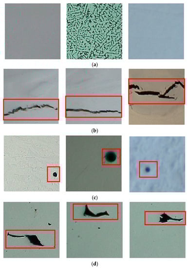
Figure 1.
Examples of laser metal deposition (LMD) build parts quality optical images: (a) good quality, (b) crack, (c) gas porosity, and (d) lack of fusion with a resolution of 224 × 224 pixels.
Table 2.
The number of images in each category.
2.3. Data Augmentation
To achieve good performance of CNN, a large number of labeled datasets are needed. As our dataset is comprised of several thousands of samples, the expansion of the dataset is necessary. Therefore, data augmentation operations [22] were applied to our original images. Each image was passed through a series transformation: random rotation from −180° to 180°, horizontal flipping, random crop, adding Gaussian noise and blur [16], as shown in Figure 2.
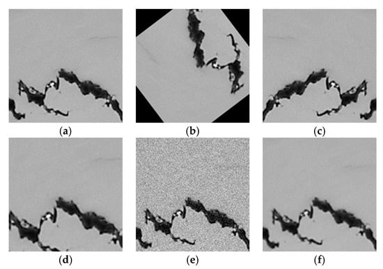
Figure 2.
Data augmentation: (a) origin image, (b) rotation, (c) flipping, (d) crop, (e) adding Gaussian noise, and (f) adding blur.
2.4. Convolutional Neural Network (CNN) Architecture
Several CNN models were explored using our dataset to obtain the optimal hyper-parameters of the model. Figure 3 presents the final schematic framework after several experiments. The overall schematic model is composed of feature extraction and classification. To make this work in a self-contained way, the fundamentals of our CNN model will be briefly described below. First, there were M depth images, Xm, and the images were scaled to 224 × 224 pixels with grayscales after the data augmentation process, and then fed into the first convolutional layer with the kernel size of 5 × 5 for feature extraction. In order to model non-linearities of the mapping between input and output, the Rectified Linear Unit (ReLU(x) = max (0,x)) [21] was used in each convolutional layer operation. Moreover, a max pooling layer of 2 × 2 was followed by each convolutional layer. The max pooling layer substituted the activation in a sub-region of the feature map with the maximum value in that region. The pooling layer downsampled the previous feature map.
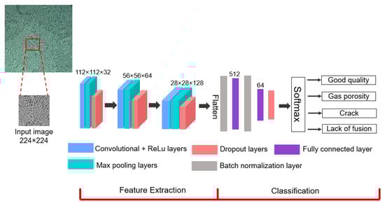
Figure 3.
Final schematic of the convolutional neural network (CNN) model for autonomous recognition of LMD build parts quality.
After the feature extraction, the classification module took the 28 × 28 × 128 feature maps and flattened them as a 512 feature vector. Then fully connected (FC) layers were applied to densify the 512 feature vector to the dimension of 64 and C, where C is the number of categories in our dataset. The vectors of C dimensions ([V1, V2, …, Vc]) were computed the predicted probability of a class using Softmax function [21] Equation (1) and transformed to the output.
where was the predicted probability of a sample Xm being class c.
During the training process of our CNN model, the difference between the true class and corresponding predicted class were calculated by the cross-entropy loss function as in Equation (2). Through the optimization of parameters in the network, our target was to minimize the loss function for the training dataset X.
2.4.1. Hyper-Parameter Tuning
The hyper-parameter is a crucial part of the CNN model and has a significant impact on the performance, such as the number of the convolutional layers, kernel size, and L2 regularization and dropout [21] parameters. To determine the optimal hyper-parameters, several architectures were built and trained. The study of hyper-parameters was based on the training and validation datasets, which is described in Section 3.1, Section 3.2 and Section 3.3.
2.4.2. Training Details
The experiments in this work were conducted with one six-core Advanced Micro Devices (AMD, Santa Clara, CA, USA) Ryzen 5 2600 processor and one Nvidia (Santa Clara, CA, USA) GeForce 1070 GPU. The code was developed in Python 3.6.8 using TensorFlow (version 1.13.1) and Keras (version 2.2.4). Some parameters were common in all experiments and are described here. A batch size of 32 and a learning rate of 1 × 10⁻⁴ were used. Each convolutional layer was followed by a max pooling layer with a filter size of 2 × 2 and a stride of 1. Batch normalization was used for centering and normalization of the images [40] and applied before the fully connected layers. An Adam optimizer [41] was used in the training process. Each network was identified with a unique Model #.
2.4.3. Evaluation Metrics
The commonly used evaluation metrics were implemented for our multiclass performance as in Equations (3)–(5).
Precision:
Recall:
F score:
In Equations (3)–(5), True Positive (TP) describes a sample from Xm from a certain class ym that is correctly classified as ym; False Positive (FP) represents a sample of Xm which does not belong to class ym but incorrectly classified as ym; False Negative (FN) is defined as a sample of Xm belonging to the class ym that is incorrectly classified as “not ym” classes. F score in Equation (5) indicates the overall performance of the precision and recall, which is their harmonic mean in the interval of [0, 1].
3. Results and Discussion
3.1. Evaluation of the CNN Architecture
Because of the complexity and parametric variation existing in the CNN models, it was not feasible to perform all possible models with their parameters, e.g., kernel size, the number of convolutional layers. Therefore, six representative CNN models with an increasing number of convolutional layers were compared to find the optimal network. The experimental results of the six CNN frameworks are tabulated in Table 3. It was shown that by increasing the depth and the number of kernels of the network, the validation accuracy changed from 74.6% to 83.8% (from Model 1 to Model 6). The accuracy and loss plots for Model 6 in Figure 4 suggested the overfitting, in which the model fit better on the training dataset than on the validation dataset. Considering the validation accuracy, the following data augmentation operations were conducted with the network used in Models 3–6.
Table 3.
Experimental results with six architectures. The convolutional layers’ parameters are denoted as “C kernel size/number of kernels”. The fully connected layers are denoted as “FC number of hidden units”. Epoch = 30, learning rate = 1 × 10⁻⁴.
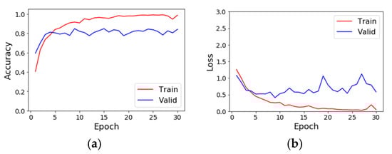
Figure 4.
(a) The accuracy and (b) the loss values of the training and validation dataset for Model 6.
3.2. Impact of Data Augmentation
Data augmentation operations were carried out on original images, and the classification performance is provided in Table 4. It was found that the validation accuracy has improved up to 5.6% compared to Table 3. It took an average of 5 min 13 s longer to train the models compared to doing so without data augmentation. Therefore, with the availability of large training datasets, the CNN models could achieve high accuracies. The following regularization was performed on the architectures of Models 5 and 6 associated with data augmentation.
Table 4.
Experimental results of Models 3–6 using data augmentation operations. The convolutional layers’ parameters are denoted as “C kernel size/number of kernels”. The fully connected layers are denoted as “FC number of hidden units”. Epoch = 30 and learning rate = 1 × 10⁻⁴.
3.3. Regularization
Regularization could be used to mitigate the problem of overfitting during the training process. The implementation of L2 regularization and dropout were explored in our study. L2 regularization applies a penalty on large framework parameters and forces them to be relatively small. Dropout is a method that randomly drops units in the network. Several combinations of L2 regularization and dropout in convolutional and fully connected layers were tested. The training time and validation accuracy of eight models were presented in Table 5. The use of L2 in the convolutional layer with a ratio of 1 × 10⁻⁵ and a dropout rate of 0.25 on all layers was demonstrated to be the most conducive for both architectures. Regarding the convolutional kernel size, the size of 5 has a 4.3% higher validation accuracy than the size of 3. Therefore, Model 11 was chosen, and the corresponding accuracy and loss plots are shown in Figure 5. It was observed that the overfitting issue was alleviated compared to Model 6 in Figure 4, but more fine tuning of regularization parameters and longer training time were needed to improve the network performance.
Table 5.
Experimental results of different L2 regularization and dropout parameters. The convolutional layers’ parameters are denoted as “C kernel size/number of kernels”. The fully connected layers are denoted as “FC number of hidden units”. Epoch = 30 and learning rate = 1 × 10⁻⁴.
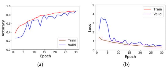
Figure 5.
(a) The accuracy and (b) the loss values of the training and validation dataset for Model 11 using data augmentation, L2 regularization, and dropout.
Model 11 was trained for the fine tuning dropout parameters with epochs of 300, and the results are listed in Table 6. Model 16 achieved a validation accuracy of 94.3% and outperformed other models. The accuracy and loss plots of the four tested models are shown in Figure 6. The learning rate was increasing until around 100–150 epochs in Figure 6a. The training and validation accuracy climbed until about 50–100 epochs and then plateaued as seen in Figure 6c,e,g, but overfitting was displayed as worse in Models 17 and 18. Thus, Model 16 was chosen as our final model that converged fast and had high validation accuracy of 94.3% with a training time of about 1 h and 46 min. The schematic architecture of Model 16 is shown in Figure 3.
Table 6.
Results of fine tuning dropout parameters. The convolutional layers’ parameters are denoted as “C kernel size/number of kernels”. The fully connected layers are denoted as “FC number of hidden units”. Epoch = 300 and learning rate = 1 × 10⁻⁴.
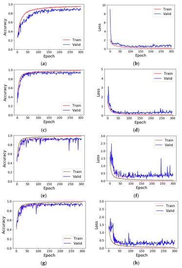
Figure 6.
Plots of accuracy and loss for (a,b) Model 15, (c,d) Model 16, (e,f) Model 17 and (g,h) Model 18. (a,c,e) and (g) are accuracy plots and (b,d,f) and (h) are loss plots.
3.4. Performance Evaluation
The performance of our final model was evaluated on the test dataset. The results of the precision recall and F score of each class are reported in Table 7. Note that the overall F score could reach above 0.9, indicating good classification performance. It took about 8.01 milliseconds to handle one image in our test process, which could be adopted for real-time inspection applications.
Table 7.
Precision, recall, and F score of the final model on the test dataset.
The classification accuracy of three different alloys in the test dataset is listed in Table 8. It is shown that the average accuracy is 91.9% (AlCoCrFeNi alloy), 91.5% (Ti-6Al-4V) and 92.7% (AISI 304 stainless steel) respectively, and the difference is ~1%. This indicates that the model can classify the defects robustly for different alloys.
Table 8.
Classification accuracy of different alloys in the test dataset.
Table 9 reports the comparison of the test accuracy of our approach and other methods whose codes are publicly available. The results were experimental on our metal AM parts quality dataset. The accuracy obtained by histogram of oriented gradients (HOG) + SVM [42] was 79.6%, while the accuracy of 89.3% was achieved using Liu’s CNN model [36]. Our approach had an accuracy of 92.1%. This could be attributed to our model being efficient in learning the internal features of the AM metal defects, which would be a benefit for our classification task.
Table 9.
The performance of classification accuracy with different methods.
3.5. Feature Visualization
To have a better understanding of what the CNN model has learned, the learned filters and the extracted feature maps are visualized in Figure 7. The 32 filters from the first convolutional layers are shown in Figure 7a. Four samples representing crack, lack of fusion, gas porosity, and good quality are present in Figure 7b–e. It seems difficult to interpret those 32 5 × 5 filters in Figure 7a, but some low-level features are extracted by reviewing the features maps in Figure 7b–e. For example, these filters were able to identify the edges of the crack, as in Figure 7b. The irregular shape of the lack of fusion was emphasized by the filters, which was different from the round shape in gas porosity. The second and the third convolutional layers are not discussed here, as they contain the high-dimensional information and make it less visually interpretable.
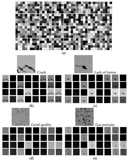
Figure 7.
Visualization of the (a) 32 learned filters of the first convolutional layers, (b) 32 feature maps for a crack sample, (c) 32 feature maps for a lack of fusion sample, (d) 32 feature maps for a good sample and (e) 32 feature maps for a gas porosity sample.
Attention maps can be obtained for a given input image with back-propagation on a CNN model. The value of each pixel on the attention map is able to reveal to what extent the same pixel on the input image makes contributions to the final output of the network [18,19]. Therefore, through the attention maps, it can intuitively analyze which part of the AM build metal images attracts the attention of the network. Figure 8 includes the AM build metallic parts profiles shown in a–d and the corresponding attention maps e–h. The defects were highlighted in the red circles and rectangles in Figure 8a–d. The bright places indicate where the CNN model focuses, as seen in Figure 8e–h, while the dark regions suggest where the network is less interested. Those maps demonstrate that the network pays attention to the defects and verify the effectiveness of our model.
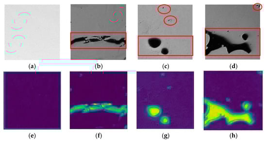
Figure 8.
(a–d) Additive manufacturing build metal parts images, (e–h) attention maps corresponding to (a–d).
3.6. Failure Case Study
The failure cases that were not correctly classified in the test dataset will be discussed in this subsection. Some incorrectly classified images are shown in Figure 9. The image shown in Figure 9a was misclassified as “good” as the dirt on the sample surface led to misclassification. The sample images shown in Figure 9b–d could be attributed to the high similarity between the gas porosity and lack of fusion, which makes it difficult to distinguish them.
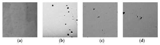
Figure 9.
Examples of wrongly classified images in the test dataset of metal additive manufacturing defects. Results highlighted in black and red indicate correct and incorrect classification results, respectively. (a) Gas—Good, (b) Gas—LoF, (c) Gas—LoF, (d) LoF—Gas.
To address the failure cases for performance improvement, some future work will be explored: (1) A variety of AM manufactured materials can be considered to be included to enlarge the dataset, e.g., ceramics, glass, polymers, and composites. (2) The architecture of the CNN models can be explored to enhance its performance.
4. Conclusions
In this paper, we presented the application of a convolutional neural network (CNN) for robust quality inspection of metal additive manufacturing (AM) parts. The Missouri S&T dataset, including optical microscope images of real-world metal AM parts were used to train and test the CNN model. This work contributed to the development of a CNN model with excellent performance in recognition of good quality, crack, gas porosities, and lack of fusion categories. To generate the appropriate model, extensive experiments were investigated on hyper-parameters including kernel size and the number of layers, data augmentation operations, and regularization. Our final model achieved an accuracy of 92.1% with 8.01 milliseconds recognition time of one image. The results indicate the promising application of the CNN method in quality inspection in the AM industry. It would be interesting to explore more CNN architectures and include a variety of materials in the future.
Author Contributions
W.C. designed and performed the experiments, wrote the manuscript; Y.Z., X.Z. and L.L. assisted the analysis; F.L. supervised the research. All the authors reviewed the manuscript. All authors have read and agreed to the published version of the manuscript.
Funding
The authors are grateful for the financial support from NSF (National Science Foundation) grants CMMI-1625736 and EEC-1937128, and Intelligent System Center (ISC) at Missouri University of Science and Technology.
Acknowledgments
The materials preparation and characterization were supported by the Materials Research Center (MRC) at Missouri University of Science and Technology. W.C. would like to thank Wenbin Li and Wenjin Tao from Missouri University of Science and Technology for their discussion and suggestions.
Conflicts of Interest
The authors declare no conflict of interest.
References
- Caggiano, A.; Zhang, J.; Alfieri, V.; Caiazzo, F.; Gao, R.; Teti, R. Machine learning-based image processing for on-line defect recognition in additive manufacturing. CIRP Ann. 2019, 68, 451–454. [Google Scholar] [CrossRef]
- Carroll, B.E.; Otis, R.A.; Borgonia, J.P.; Suh, J.O.; Dillon, R.P.; Shapiro, A.A.; Hofmann, D.C.; Liu, Z.K.; Beese, A.M. Functionally graded material of 304L stainless steel and inconel 625 fabricated by directed energy deposition: Characterization and thermodynamic modeling. Acta Mater. 2016, 108, 46–54. [Google Scholar] [CrossRef]
- Reichardt, A.; Dillon, R.P.; Borgonia, J.P.; Shapiro, A.A.; McEnerney, B.W.; Momose, T.; Hosemann, P. Development and characterization of Ti-6Al-4V to 304L stainless steel gradient components fabricated with laser deposition additive manufacturing. Mater. Des. 2016, 104, 404–413. [Google Scholar] [CrossRef]
- Huang, C.; Zhang, Y.; Vilar, R.; Shen, J. Dry sliding wear behavior of laser clad TiVCrAlSi high entropy alloy coatings on Ti-6Al-4V substrate. Mater. Des. 2012, 41, 338–343. [Google Scholar] [CrossRef]
- Cui, W.; Karnati, S.; Zhang, X.; Burns, E.; Liou, F. Fabrication of AlCoCrFeNi high-entropy alloy coating on an AISI 304 substrate via a CoFe2Ni intermediate layer. Entropy 2019, 21, 2. [Google Scholar] [CrossRef]
- Åkerfeldt, P.; Antti, M.L.; Pederson, R. Influence of microstructure on mechanical properties of laser metal wire-deposited Ti-6Al-4V. Mater. Sci. Eng. A 2016, 674, 428–437. [Google Scholar] [CrossRef]
- Åkerfeldt, P.; Pederson, R.; Antti, M.L. A fractographic study exploring the relationship between the low cycle fatigue and metallurgical properties of laser metal wire deposited Ti-6Al-4V. Int. J. Fatigue 2016, 87, 245–256. [Google Scholar] [CrossRef]
- Sun, G.; Zhou, R.; Lu, J.; Mazumder, J. Evaluation of defect density, microstructure, residual stress, elastic modulus, hardness and strength of laser-deposited AISI 4340 steel. Acta Mater. 2015, 84, 172–189. [Google Scholar] [CrossRef]
- Taheri, H.; Rashid Bin, M.; Shoaib, M.; Koester, L.; Bigelow, T.; Collins, P.C. Powder-based additive manufacturing—A review of types of defects, generation mechanisms, detection, property evaluation and metrology. Int. J. Addit. Subtract. Mater. Manuf. 2017, 1, 172–209. [Google Scholar] [CrossRef]
- Li, W.; Martin, A.J.; Kroehler, B.; Henderson, A.; Huang, T.; Watts, J.; Hilmas, G.E.; Leu, M.C. Fabricating Functionally Graded Materials by Ceramic on-Demand Extrusion with Dynamic Mixing. In Proceedings of the 29th Annual International Solid Freeform Fabrication Symposium, Austin, TX, USA, 13–15 August 2018; pp. 1087–1099. [Google Scholar]
- Ahsan, M.N.; Pinkerton, A.J.; Moat, R.J.; Shackleton, J. A comparative study of laser direct metal deposition characteristics using gas and plasma-atomized Ti-6Al-4V powders. Mater. Sci. Eng. A 2011, 528, 7648–7657. [Google Scholar] [CrossRef]
- Li, W.; Ghazanfari, A.; McMillen, D.; Leu, M.C.; Hilmas, G.E.; Watts, J. Characterization of zirconia specimens fabricated by ceramic on-demand extrusion. Ceram. Int. 2018, 44, 12245–12252. [Google Scholar] [CrossRef]
- Azimi, S.M.; Britz, D.; Engstler, M.; Fritz, M.; Mücklich, F. Advanced steel microstructural classification by deep learning methods. Sci. Rep. 2018, 8, 2128. [Google Scholar] [CrossRef] [PubMed]
- Guan, S. Strip Steel Defect Detection Based on Saliency Map Construction Using Gaussian Pyramid Decomposition. ISIJ Int. 2015, 55, 1950–1955. [Google Scholar] [CrossRef]
- Barua, S.; Liou, F.; Newkirk, J.; Sparks, T. Vision-based defect detection in laser metal deposition process. Rapid Prototyp. J. 2014, 20, 77–85. [Google Scholar] [CrossRef]
- Yi, L.; Li, G.; Jiang, M. An End-to-End Steel Strip Surface Defects Recognition System Based on Convolutional Neural Networks. Steel Res. Int. 2017, 88, 176–187. [Google Scholar] [CrossRef]
- Tao, W.; Leu, M.C.; Yin, Z. American Sign Language alphabet recognition using Convolutional Neural Networks with multiview augmentation and inference fusion. Eng. Appl. Artif. Intell. 2018, 76, 202–213. [Google Scholar] [CrossRef]
- Li, K.; Wu, Z.; Peng, K.C.; Ernst, J.; Fu, Y. Tell Me Where to Look: Guided Attention Inference Network. In Proceedings of the IEEE Computer Society Conference on Computer Vision and Pattern Recognition, Salt Lake City, UT, USA, 18–22 June 2018; pp. 9215–9223. [Google Scholar]
- Zhou, B.; Khosla, A.; Lapedriza, A.; Oliva, A.; Torralba, A. Learning Deep Features for Discriminative Localization. In Proceedings of the IEEE Computer Society Conference on Computer Vision and Pattern Recognition, Las Vegas, NV, USA, 27–30 June 2016; pp. 2921–2929. [Google Scholar]
- Wang, T.; Chen, Y.; Qiao, M.; Snoussi, H. A fast and robust convolutional neural network-based defect detection model in product quality control. Int. J. Adv. Manuf. Technol. 2018, 94, 3465–3471. [Google Scholar] [CrossRef]
- Lecun, Y.; Bengio, Y.; Hinton, G. Deep learning. Nature 2015, 521, 436–444. [Google Scholar] [CrossRef]
- Krizhevsky, A.; Sutskever, I.; Hinton, G.E. ImageNet classification with deep convolutional neural networks. Adv. Neural Inf. Process. Syst. 2012, 1097–1105. [Google Scholar] [CrossRef]
- Qi, X.; Chen, G.; Li, Y.; Cheng, X.; Li, C. Applying Neural-Network-Based Machine Learning to Additive Manufacturing: Current Applications, Challenges, and Future Perspectives. Engineering 2019, 5, 721–729. [Google Scholar] [CrossRef]
- Gaja, H.; Liou, F. Defect classification of laser metal deposition using logistic regression and artificial neural networks for pattern recognition. Int. J. Adv. Manuf. Technol. 2018, 94, 315–326. [Google Scholar] [CrossRef]
- Khanzadeh, M.; Chowdhury, S.; Marufuzzaman, M.; Tschopp, M.A.; Bian, L. Porosity prediction: Supervised-learning of thermal history for direct laser deposition. J. Manuf. Syst. 2018, 47, 69–82. [Google Scholar] [CrossRef]
- Gobert, C.; Reutzel, E.W.; Petrich, J.; Nassar, A.R.; Phoha, S. Application of supervised machine learning for defect detection during metallic powder bed fusion additive manufacturing using high resolution imaging. Addit. Manuf. 2018, 21, 517–528. [Google Scholar] [CrossRef]
- DeCost, B.L.; Jain, H.; Rollett, A.D.; Holm, E.A. Computer Vision and Machine Learning for Autonomous Characterization of AM Powder Feedstocks. JOM 2017, 69, 456–465. [Google Scholar] [CrossRef]
- Venegas-Barrera, C.S.; Manjarrez, J. Visual Categorization with Bags of Keypoints. In Proceedings of the Workshop on Statistical Learning in Computer Vision, ECCV, Prague, Czech Republic, 11–14 May 2004; pp. 1–22. [Google Scholar]
- Zhang, J.; Lek, M.M.; Lazebnik, S.; Schmid, C. Local Features and Kernels for Classification of Texture and Object Categories: A Comprehensive Study. Int. J. Comput. Vis. 2007, 73, 213–238. [Google Scholar] [CrossRef]
- DeCost, B.L.; Francis, T.; Holm, E.A. Exploring the microstructure manifold: Image texture representations applied to ultrahigh carbon steel microstructures. Acta Mater. 2017, 133, 30–40. [Google Scholar] [CrossRef]
- Chowdhury, A.; Kautz, E.; Yener, B.; Lewis, D. Image driven machine learning methods for microstructure recognition. Comput. Mater. Sci. 2016, 123, 176–187. [Google Scholar] [CrossRef]
- Kondo, R.; Yamakawa, S.; Masuoka, Y.; Tajima, S.; Asahi, R. Microstructure recognition using convolutional neural networks for prediction of ionic conductivity in ceramics. Acta Mater. 2017, 141, 29–38. [Google Scholar] [CrossRef]
- Wen, S.; Chen, Z.; Li, C. Vision-based surface inspection system for bearing rollers using convolutional neural networks. Appl. Sci. 2018, 8, 2565. [Google Scholar] [CrossRef]
- Tao, X.; Zhang, D.; Ma, W.; Liu, X.; Xu, D. Automatic metallic surface defect detection and recognition with convolutional neural networks. Appl. Sci. 2018, 8, 1575. [Google Scholar] [CrossRef]
- Wei, R.; Bi, Y. Research on Recognition Technology of Aluminum Profile Surface Defects Based on Deep Learning. Materials 2019, 12, 1681. [Google Scholar] [CrossRef] [PubMed]
- Zhu, H.; Ge, W.; Liu, Z. Deep Learning-Based Classification of Weld Surface Defects. Appl. Sci. 2019, 9, 3312. [Google Scholar] [CrossRef]
- Liu, Y.; Xu, K.; Xu, J. Periodic Surface Defect Detection in Steel Plates Based on Deep Learning. Appl. Sci. 2019, 9, 3127. [Google Scholar] [CrossRef]
- Azarniya, A.; Colera, X.G.; Mirzaali, M.J.; Sovizi, S.; Bartolomeu, F.; St Weglowski, M.K.; Wits, W.W.; Yap, C.Y.; Ahn, J.; Miranda, G.; et al. Additive manufacturing of Ti–6Al–4V parts through laser metal deposition (LMD): Process, microstructure, and mechanical properties. J. Alloys Compd. 2019, 804, 163–191. [Google Scholar] [CrossRef]
- Yan, L.; Cui, W.; Newkirk, J.W.; Liou, F.; Thomas, E.E.; Baker, A.H.; Castle, J.B. Build Strategy Investigation of Ti-6Al-4V Produced Via a Hybrid Manufacturing Process. JOM 2018, 70, 1706–1713. [Google Scholar] [CrossRef]
- Ioffe, S.; Szegedy, C. Batch normalization: Accelerating deep network training by reducing internal covariate shift. In Proceedings of the 32nd International Conference on Machine Learning (ICML 2015), Lille, France, 6–11 July 2005; International Machine Learning Society (IMLS), 2015; Volume 1, pp. 448–456. [Google Scholar]
- Kingma, D.P.; Ba, J.L. Adam: A method for stochastic optimization. In Proceedings of the International Conference on Learning Representations (ICLR), San Diego, CA, USA, 7–9 May 2015. [Google Scholar]
- Ding, S.; Liu, Z.; Li, C. AdaBoost learning for fabric defect detection based on HOG and SVM. In Proceedings of the 2011 International Conference on Multimedia Technology (ICMT), Hangzhou, China, 26–28 July 2011; pp. 2903–2906. [Google Scholar]


© 2020 by the authors. Licensee MDPI, Basel, Switzerland. This article is an open access article distributed under the terms and conditions of the Creative Commons Attribution (CC BY) license (http://creativecommons.org/licenses/by/4.0/).