Article

Time–Frequency Attribute Analysis of Channel 1 Data of Lunar Penetrating Radar

1
College of Geo-exploration Science and Technology, Jilin University, Changchun 130026, China
2
Ministry of Land and Resources Key Laboratory of Applied Geophysics, Jilin University, Changchun 130026, China
*
Authors to whom correspondence should be addressed.
Appl. Sci. 2020, 10(2), 535; https://doi.org/10.3390/app10020535
Submission received: 18 December 2019 / Revised: 8 January 2020 / Accepted: 9 January 2020 / Published: 10 January 2020
(This article belongs to the Special Issue Remote Sensing and Geoscience Information Systems in Applied Sciences)

Abstract

:
The Lunar Penetrating Radar (LPR) carried by the Chang’E-3 (CE-3) and Chang’E-4 (CE-4) mission plays a very important role in lunar exploration. The dual-frequency radar on the rover (DFR) provides a meaningful opportunity to detect the underground structure of the CE-3 landing site. The low-frequency channel (channel 1) maps the underground structure to a depth of several hundred meters, while the high-frequency channel (channel 2) can observe the stratigraphic structure of gravel near the surface. As the low-frequency radar image is troubled by unknown noise, time–frequency analysis of a single trace is applied. Then, a method named complete ensemble empirical mode decomposition (CEEMD) is conducted to decompose the channel 1 data, and the Hilbert transform gives us the chance for further data analysis. Finally, combined with regional geology, previous studies, and channel 2 data, a usability analysis of LPR channel 1 data provides a reference for the availability of the CE-4 LPR data.

1. Introduction

Exploration of the lunar subsurface structure is a powerful force for the analysis of the stratigraphic thickness, time, and contact relationships, which exert a vital role not only on theorizing the evolution of the subsurface structure, but also on estimating the total resources of the lunar subsurface.
In order to detect the shallow geological structure of the moon, spaceborne radar and synthetic aperture radar (SAR) are mainly used. As early as 1972, Apollo 17 carried out on-board radar detection [1]. It operated at 5, 15, and 150 MHz. In addition, it mainly detected the underground geological structure of the moon. Since 20 November 2007, the Lunar-Radar Sounder (LRS) on Japan’s Kaguya probes (SELENE) has been surveying the moon underground. The LRS uses the high-frequency (HF) band (5 MHz) to enable the acquisition of subsurface data at depths of several kilometers [2]. The small SAR was launched on the moon in September 2007 and it carried out the Indian Chandrayaan mission. It mapped the scattering characteristics of the moon’s pole and determined the existence and extent of polar ice [3,4]. The Mini-RF instrument on the Lunar Reconnaissance Orbiter (LRO) is a SAR, and it works with bistatic radar from the Arecibo Observatory to conduct data analysis of the region. The results show that there may be near-surface sediments of water ice [4,5].
Unlike the spaceborne radar described above, the lunar radar on Chang’E-3 (CE-3) is a field instrument for underground structure detection [6]. The dual-frequency radar (DFR) offers a great opportunity to map underground structures to depths of a few hundred meters from the CH-1 and its near-surface stratigraphic structure re-aggregates from the CH-2 [7] of Mare Imbrium.
The Yutu rover (YR) landed at a height of 340.4875° E, 44.1189° N in a new area that had never been surveyed in the largest basin, the Mare Imbrium. Ancient basalts and young basalts are distributed here, and the last volcanic activity also stopped here [8]. The CE-3 Lunar Penetrating Radar (LPR) data provide a new perspective for analyzing subsurface structures. In the beginning, the LPR data primary results were put forward by the National Astronomical Observatory of the Chinese Academy of Sciences (NAOC) [9]. The preliminary analysis of LPR, especially CH-1, showed that there are nine underground layers from the surface to a depth of about 360 m [6]. The existence of three basaltic areas detected by the LPR is the same as the distribution of the three major basaltic areas in Mare Imbrium [10,11,12,13,14]. By processing the original CH-2 data, the near-surface structure was inferred. The parameters of cemented carbide were calculated by Dong et al. [15] and Zhang et al. [16]. Wang et al. [17] and Zhang et al. [18] developed a new method for processing CH-2 data. Hu et al. proposed a rock extraction method by using local similarity constraints to realize rock location and quantitative analysis [19].
The basis for interpretation when using CH-1 data is its credibility. However, Li et al. demonstrated some false reflectors in the CH-1 data [20]. In order to analyze and decompose the CH-1 data, an analysis method that can be used in nonlinear data is necessary.
In recent years, empirical mode decomposition (EMD) [21] has developed into a data analysis method. EMD has demonstrated appropriate versatility in the application of signals for extracting from random data with a complex noise environment. Although EMD has proven to be useful, it still has some unresolved difficulties. The main disadvantage of EMD is the constant appearance of pattern blending. Signals of different scales can be combined into an intrinsic mode function (IMF).
In order to conquer the frequent occurrence of pattern mixing, a new method of noise assisted data analysis (NADA) has been proposed. Its name is ensemble EMD (EEMD) [22]. The core idea of this method is to average the results of EMD and apply it to the original signal. The EEMD method can solve the pattern blending, but it creates a new pattern.
In the use of complete ensemble empirical mode decomposition (CEEMD) [23], all the stages after decomposition will add some specific noise. Next, a unique residue is calculated to obtain each pattern. The final decomposition is finished, and the error is negligible. Compared to EMD and EEMD, CEEMD provides a better mode spectral separation and fewer screening iterations while also reducing computational costs.
As mentioned by Li et al. [20], the signal-to-noise ratio (SNR) of the CH-1 data is extremely low and there are many false reflectors in the CH-1 data. It is important to be able to extract useful information from the CH-1 data. In order to analyze and decompose the CH-1 data, an analysis method, which combines CEEMD and time–frequency analysis, is developed. This method can not only analyze the LPR CH-1 data of CE-3, but also provide an analysis method for the subsequent Chang’E-4 (CE-4) radar data.
In this paper, time–frequency analysis is applied to the troubled data. Then, CEEMD is conducted to decompose the channel 1 data, and the Hilbert transform gives us the chance for further data analysis. Furthermore, combined with geological information, the previous summary, and the channel 2 data, usability analysis of the LPR channel 1 data has been conducted, which can provide a reference for the usability of the CE-4 LPR data.

2. Materials and Methods

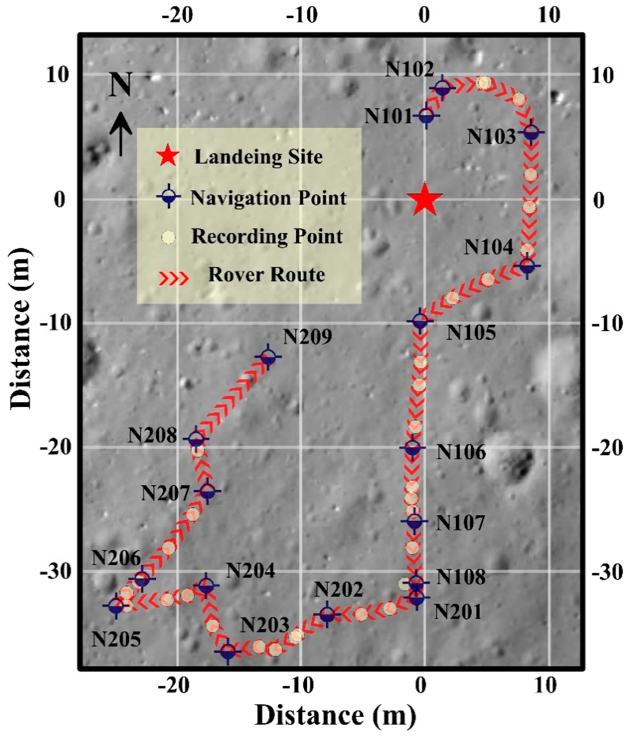
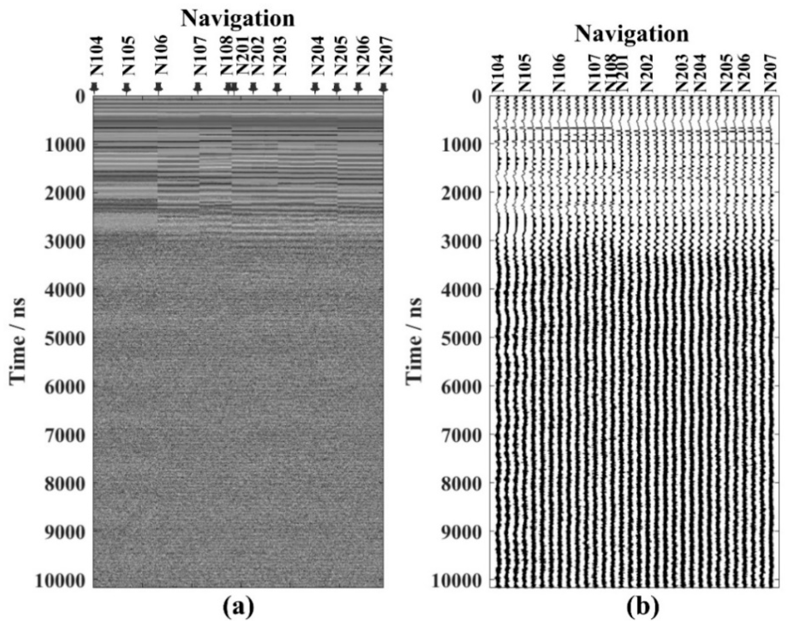
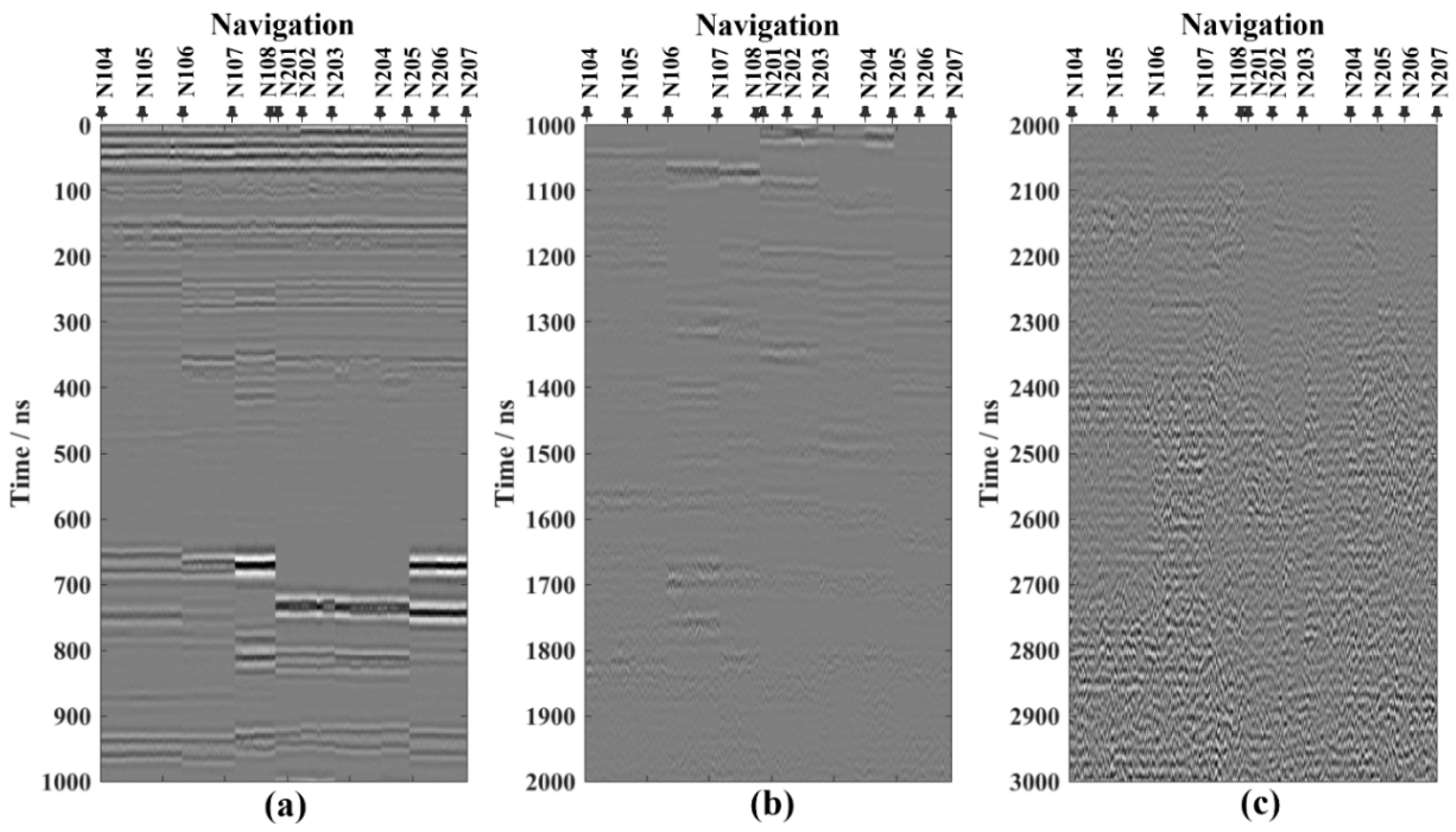
2.1. Data Explanation and Preprocessing
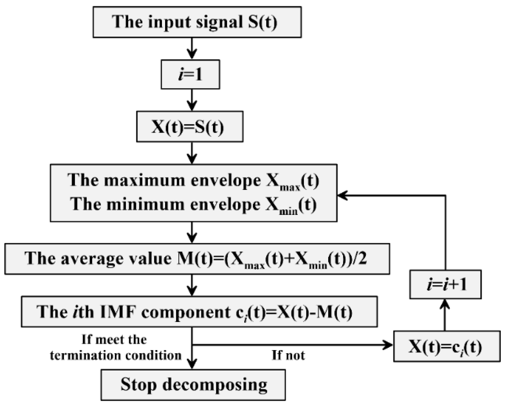
The YR launched by CE-3 was the first to land on the moon after the Soviet Union in 1976. Specifically, the YR used it to detect the surface of the landing site on the north side of the mare and several instruments in the ground. Its trajectory stretched to 114.8 m near the sinus (Figure 1). In this installment, the data description and pretreatment of the LPR CH-1 data will be introduced.
The DFR on the YR offers a meaningful chance to map the underground structure about several hundred meters deep from the CH-1 (60 MHz) and its stratigraphic structure near the surface from the CH-2 (500 MHz). For the underground structure, the CH-1 data are selected. According to the recording parameters, real conditions, and data condition, a set of LPR data pretreatment procedures (Table 1) was projected. The data can be preprocessed to access the CH-1 image (Figure 2).
There are many kinds of space electromagnetic waves on the moon; the terrain of the moon is very complex under the adverse circumstances, so the signal-to-noise ratio (SNR) of LPR data is low. The repeated gathers of each stop point are superimposed, the purpose of which is to improve the SNR of the single trace at the waypoint [24], and provide more accurate and reasonable one-dimensional data for the subsequent analysis of the frequency-domain (FD) and the time–frequency domain (TFD).
In this paper, several analysis and processing methods are utilized, for example, the Fourier transform, short-time Fourier transform, CEEMD, and Hilbert transform. The Fourier transform (FT) and short-time Fourier transform (STFT) are commonly used as data analysis methods, the principle of which will not be repeated here. This section mainly introduces the CEEMD and Hilbert transform.

2.2. CEEMD

CEEMD comes from EMD and EEMD. The EMD method resolves a given signal into a series of IMFs. These IMFs are components that satisfy certain conditions. The reconstructed original signal is [22]
x = i = 1 n c i + r n ,
where c i is the ith IMF and r n is the residue of data x after n IMFs are extracted. The decomposition flowchart of EMD is shown in Figure 3. The termination conditions of the EMD in the figure are: (1) The number of extreme points is the same as or, at most, one of the zero crossings; (2) the average value of the envelope defined by the local extremum at any point is zero.
As mentioned above, the main disadvantage of EMD is the frequent occurrence of mode overlap, which is defined as a single IMF composed of signals of different scales, or a signal of likeness scale in varying IMF components. In order to overcome the frequent appearance of mode overlap, several new noise-assisted data analysis methods are proposed, such as variational mode decomposition (VMD) [25] and ensemble EMD (EEMD) [22]. The EEMD method can be expressed as follows [23]:
  • Generate
    x i [ n ] = x [ n ] + w i [ n ] ,
    where w i [ n ] (i = 1, …, I) are different implementations of white Gaussian noise,
  • Each x i [ n ] (i = 1, …, I) is fully resolved by EMD to get their modes I M F k i [ n ] , where k = 1, K represents the modes,
  • Set up I M F ¯ k to be the k-th pattern of x [ n ] , obtained as the corresponding average I M F k i [23]:
    I M F ¯ k [ n ] = 1 I i = 1 I I M F k i [ n ] .
The resulting decomposition of EEMD solves the problem of mode mixing; however, it introduces new ones. In the technique of CEEMD, the decomposition mode will be recorded as I M F ˜ k and be proposed to count a unique first residue as
r 1 [ n ] = x [ n ] I M F ˜ 1 [ n ] .
I M F ˜ 1 [ n ] is obtained in the same way as EEMD. Then, calculate the first EMD mode over aggregate r 1 [ n ] plus various realizations of a given noise, obtaining I M F ˜ 2 through averaging. The next residue can be defined as r 2 [ n ] = r 1 [ n ] I M F ˜ 2 [ n ] . The rest of the mode continues working until the requirements are met.
First, we define an operator E j ( ) , which, given a signal, produces the j-th mode from EMD [23]. w i is the white noise with N ( 0 , 1 ) . If x [ n ] is the target datastore, the method can be described by the following algorithm [23]:
  • Disintegrate by EMD I realizations x [ n ] + ε 0 w i [ n ] to obtain their first modes and calculate
    I M F ˜ 1 [ n ] = 1 I i = 1 I I M F 1 i [ n ] = I M F ¯ 1 [ n ] .
  • In the first phase (k = 1), obtain the first residue as in Equation (4).
  • Decompose realizations r 1 [ n ] + ε 1 E 1 ( w i [ n ] ) , i = 1, …, I, until their first EMD mode and define the second mode [23]:
    I M F ˜ 2 [ n ] = 1 I i = 1 I E 1 ( r 1 [ n ] + ε 1 E 1 ( w i [ n ] ) ) .
  • For k = 2, …, K, calculate the k-th residue [23]:
    r k [ n ] = r ( k 1 ) [ n ] I M F ˜ k [ n ] .
  • Decompose realizations r k [ n ] + ε k E k ( w i [ n ] ) , i = 1, …, I, until their first EMD mode and define the (k + 1)-th mode as [23]
    I M F ˜ ( k + 1 ) [ n ] = 1 I i = 1 I E 1 ( r k [ n ] + ε k E k ( w i [ n ] ) ) .
  • Go to step 4 to continue to get the next k.
Repeat steps 4–6. The direct residual part cannot be further decomposed, and the final residue satisfies [23]
R [ n ] = x [ n ] k = 1 K I M F k ˜ ,
K is the total number of modes. Therefore, the given signal x [ n ] can be written as
x [ n ] = k = 1 K I M F k ˜ + R [ n ] .
Equation (10) indicates that the data decomposition has been completed and the original data can be reconstructed.

2.3. Hilbert Transform

After introducing the algorithm of CEEMD, we describe the principle of the Hilbert transform.
For any time series X ( t ) , we can get its Hilbert transform result:
Y ( t ) = 1 π X ( τ ) t τ d τ .
The Hilbert inverse transformation is
X ( t ) = H 1 [ Y ( t ) ] = 1 π t Y ( t ) = 1 π Y ( t τ ) τ d τ = 1 π Y ( t + τ ) τ d τ .
For a real signal X ( t ) , there are many kinds of complex methods, and it is the simplest and most effective to obtain the analytical signal by the Hilbert transform method. Assuming that the Hilbert transform of X ( t ) is Y ( t ) , the expression of the parsed signal is
Z ( t ) = X ( t ) + i Y ( t ) = a ( t ) e i θ ( t ) ,
where a ( t ) and θ ( t ) are the instantaneous amplitude and phase of the signal, respectively, and they can be written in the following form:
a ( t ) = X 2 ( t ) + Y 2 ( t ) ,
θ ( t ) = tan 1 X ( t ) Y ( t ) .
The signal’s instantaneous frequency can be obtained by deriving the instantaneous phase:
ω ( t ) = d θ ( t ) d t .
Unlike the Fourier transform, a and ω in the equation are not constant, but a function of time, so the Hilbert spectrum can characterize the temporal variation of a data sequence; the instantaneous frequency is relative to the analytical signal, which is the analytical signal phase.
The frequency obtained by the signal FT reflects the distribution characteristics of the signal with time, and the frequency of the signal with time cannot be obtained. The instantaneous frequency reflects the frequency of the signal at a certain time, which can better describe the characteristics of the signal. This is also the main difference between them. The Hilbert transform can only deal with the stationary signal of a single frequency, which has great limitations for non-stationary signals with multiple frequencies at a certain time. Therefore, the Hilbert transform must meet some constraints in the application to obtain a physical instantaneous frequency.

3. Results

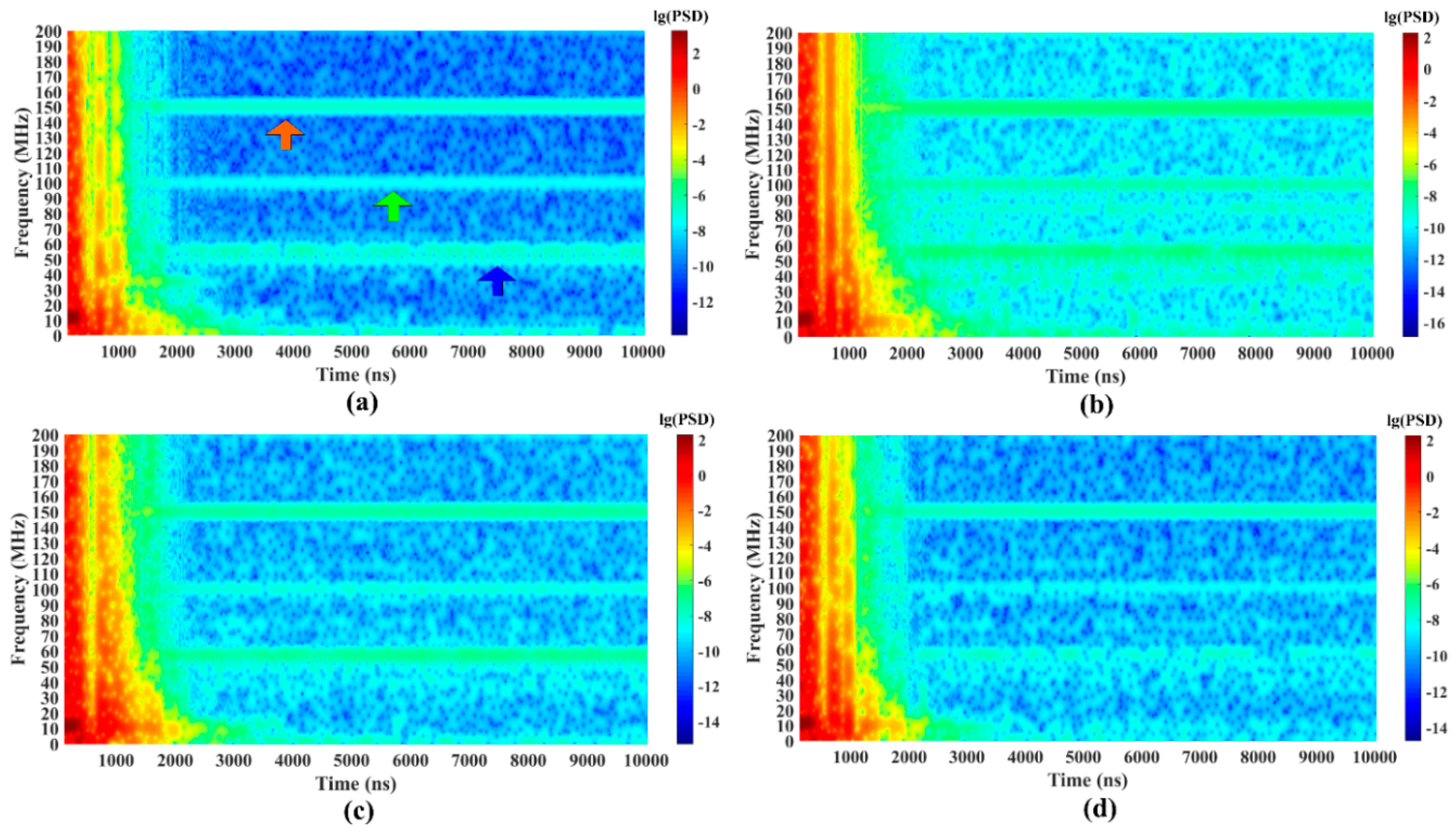
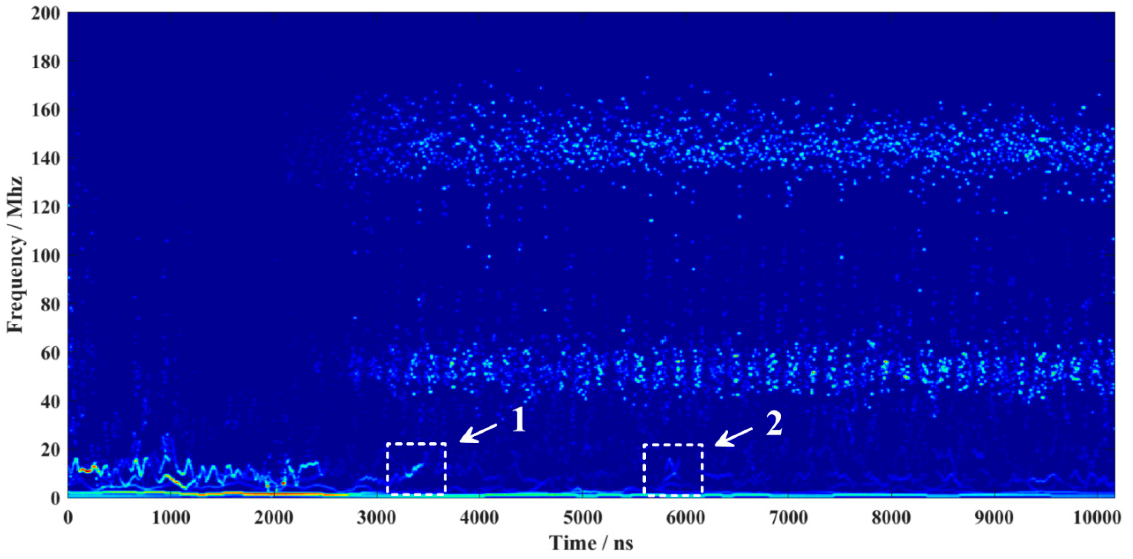
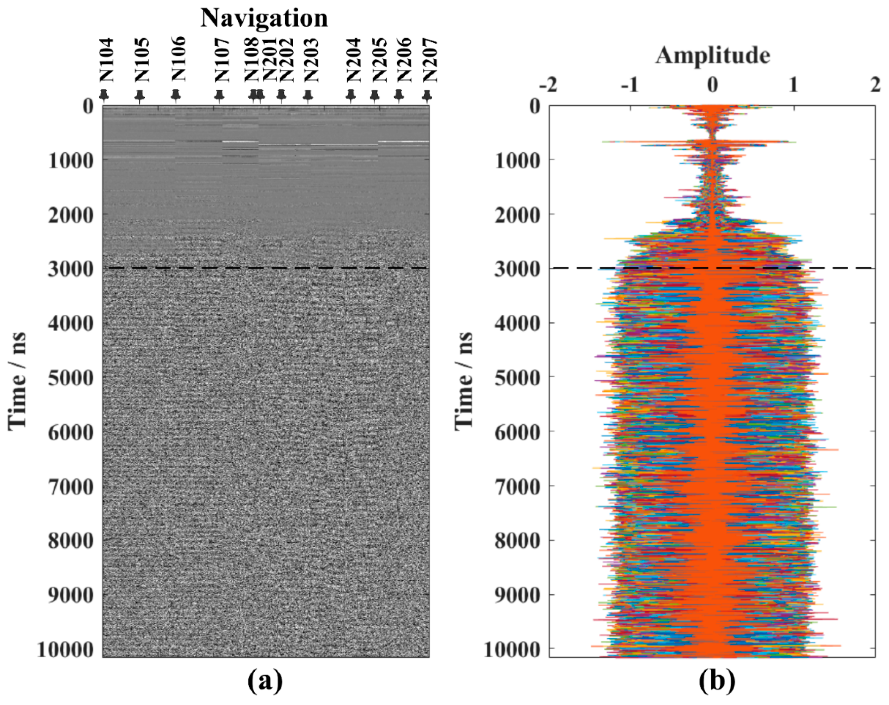
3.1. Analysis in Frequency Domain and the Time–Frequency Domain

The FT and the STFT are performed to obtain the frequency spectrum (Figure 4) and the time–frequency spectrum (Figure 5) (et al., N104, N106, N202, and N206, for examples), and, thus, the time–frequency spectra will expose the issue and the kind of processing that should be done.
It can be seen from the frequency spectra of the sample traces (Figure 4) that in the frequency domain, the maximum energy of all sample gathers is around 12 MHz (as indicated by the arrow), whereas at around 60 MHz (the center frequency of CH-1), the energy is not prominent.
Take a look at the time–frequency spectra of the sample traces:
(1)
As the arrows in the N104 time–frequency spectrum of STFT show, there are 150, 100, and 60 MHz electromagnetic energies in the data throughout the entire time delay. Obviously, the energies at 150 and 100 MHz are not the transmitting signals. The electromagnetic energies at those frequencies may have come from the lunar space or the instrument (needs further research).
(2)
Compared to the shallow signal, the energy of the deep electromagnetic signal is very weak. Gain should be processed to highlight the deep information (Figure 6).
(3)
Both the energies of the high-frequency and low-frequency information in the shallow part are strong. As the time delay increases, high-frequency energy is absorbed, and only some low-frequency information is left. For this kind of nonlinear frequency aliasing phenomenon, a nonlinear decomposition method must be processed.

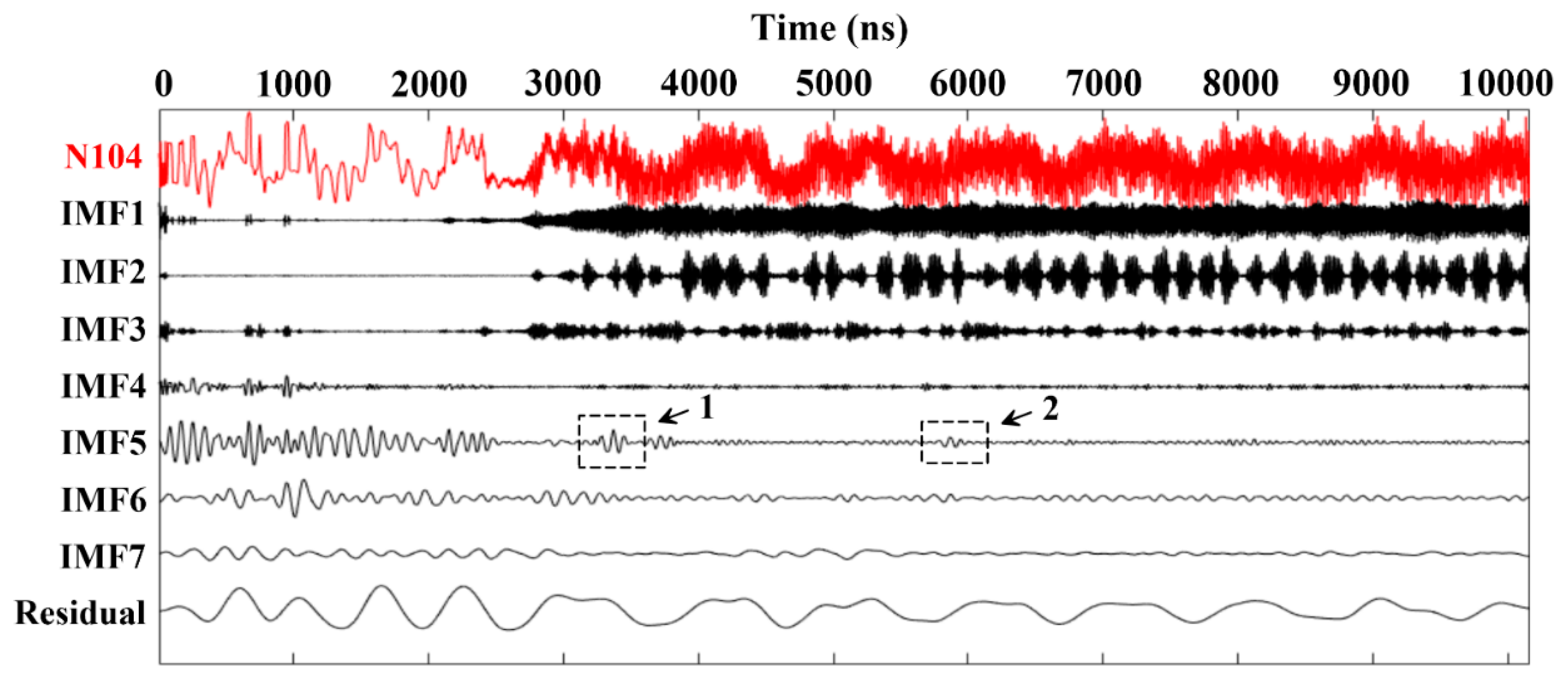
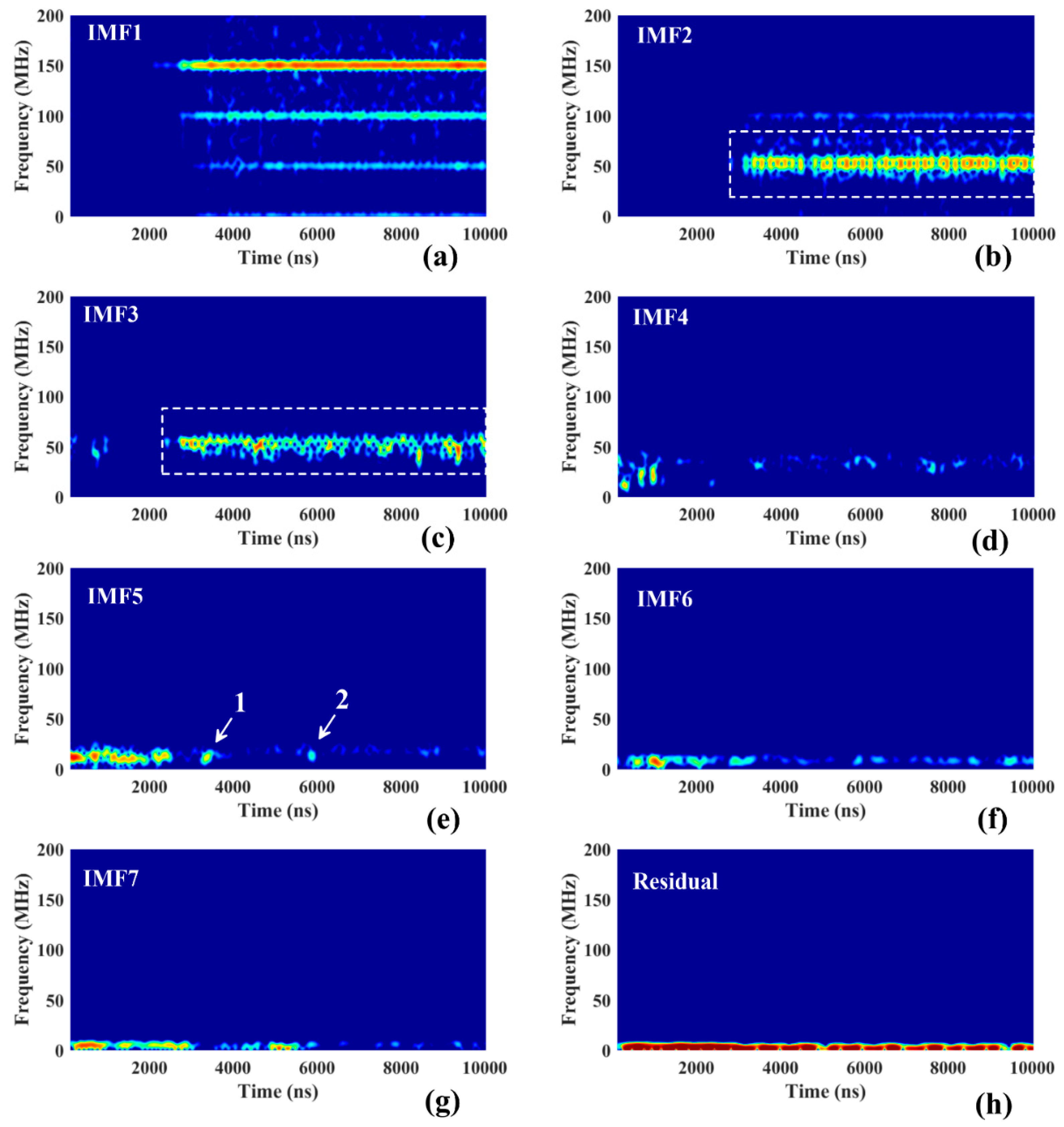
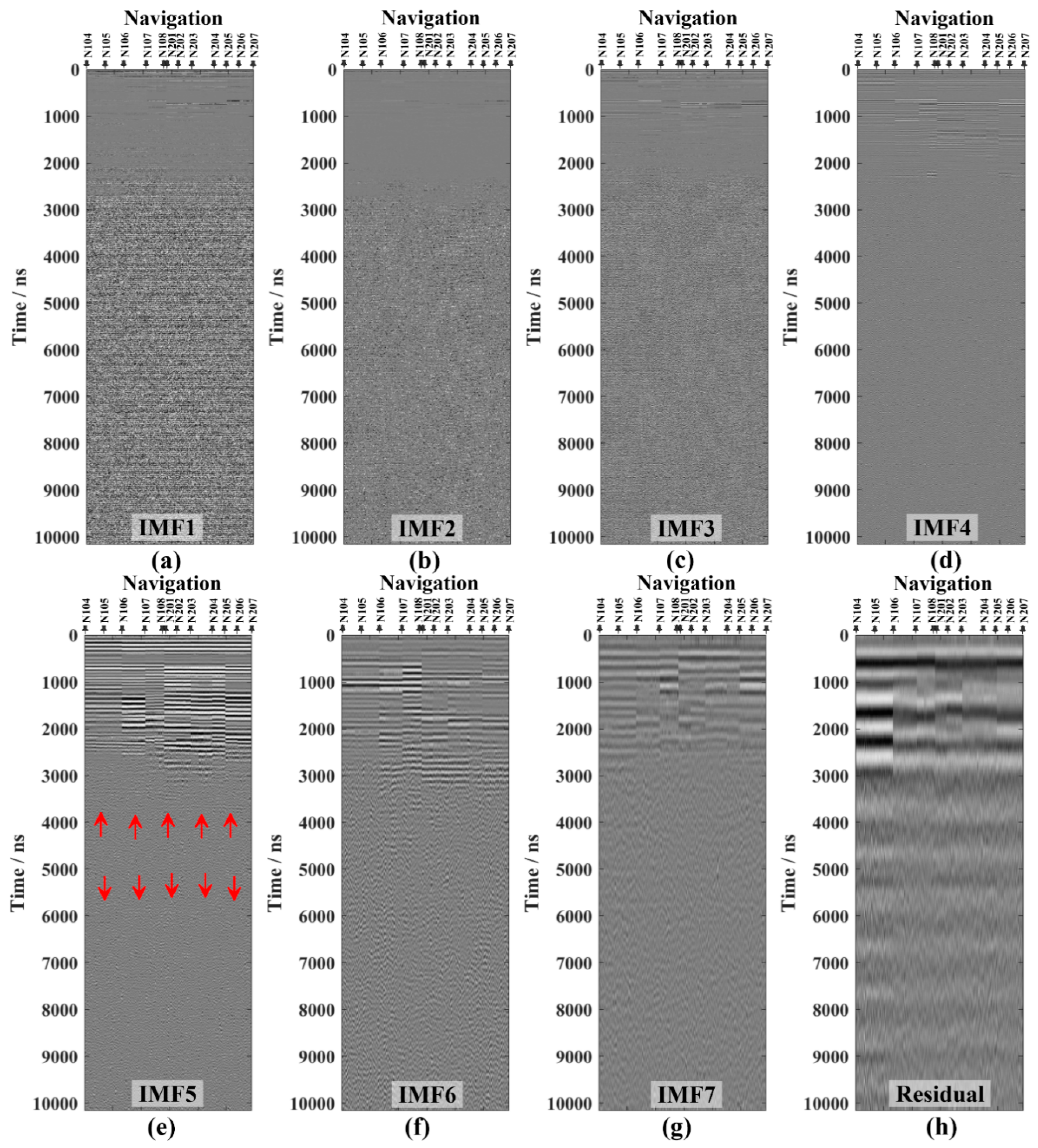
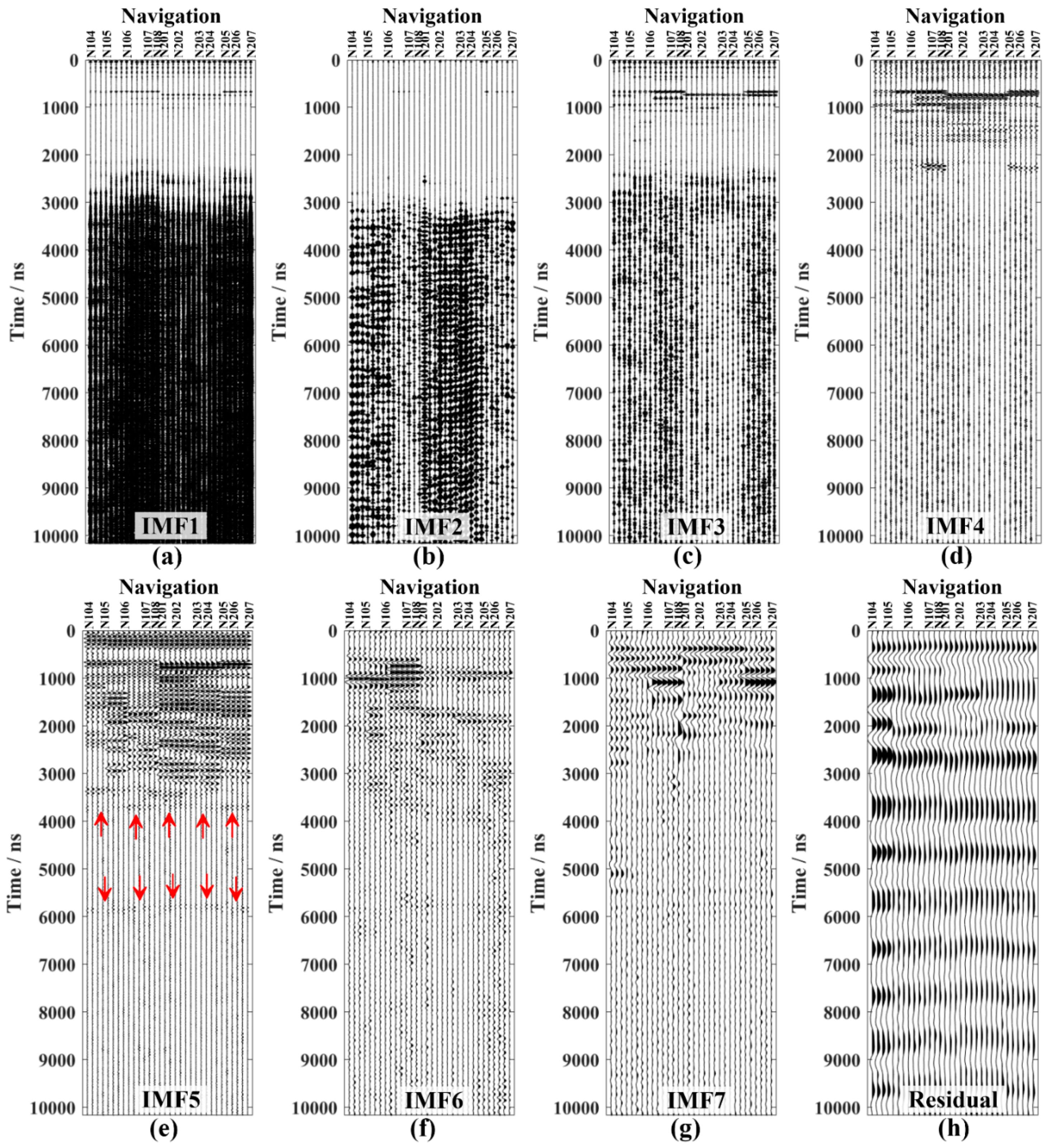
3.2. CEEMD of the Trace at N104
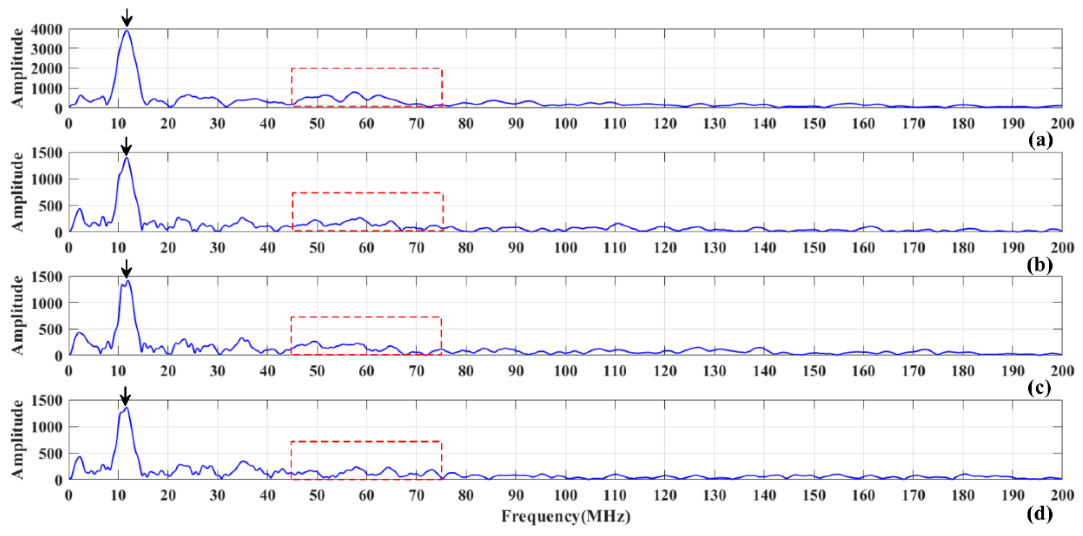
In terms of the N104 trace, CEEMD is performed (Figure 7). The noise standard deviation is set to be 0.2. The number of realizations is 200 and the maximum number of sifting iterations allowed is 2000. The N104 trace is divided into seven IMFs and one residual.
After decomposing the trace at N104, in order to observe the time–frequency information of the data in each component, we performed a short-time Fourier transform for each component (Figure 8). Analyze each component one by one:
(1)
In the STFT spectrum of the IMF1 component, energy is concentrated mainly at 150 MHz, and a small amount of energy is at 100 and 60 MHz; this component can be considered a high-frequency noise component.
(2)
In the STFT spectrum of the IMF2 and IMF3 components, the main energy is collected near 60 MHz, and some of the energy scattered around it is considered to be the component containing the useful signal.
(3)
The main energy in the STFT spectrum of the IMF4 component is collected near 30 MHz, which is considered to be a lower-frequency noise component.
(4)
Among the IMF components, IMF5 is worthy of attention. Two obvious energy information are observed from the component curve (in the IMF5 curve in Figure 7) and its STFT spectrum (Figure 8e), which are around 3500 and 5800 ns, respectively. The reflection of these two positions was used for reflection in the articles by Xiao et al. [6] and Zhang et al. [10], but it can be seen from the STFT spectrum that the frequency is between 10 and 15 MHz, and it is quite different from the center frequency of the transmitter. Li et al. also used the S transform and LPR ground data to verify the trap of these two pitfalls [20]. In summary, the IMF5 component is considered to be the unusable component.
(5)
The STFT spectra of IMF5, IMF6, and IMF7 and the residual component show that the energy is collected below 10 MHz, which is a low-frequency unwanted component.
On the other hand, from the Hilbert spectrum of IMFs at N104 (Figure 9), it can be seen that the energy in the shallow part is mainly distributed in the low-frequency IMF components below 20 MHz. The deep part mainly includes three parts, a high-frequency IMF component of 150 MHz, an IMF component of 60 MHz, which is consistent with the transmission frequency, and a low-frequency pitfall component of 20 MHz or less. Here again, an aliasing component around 3500 and 5800 ns can be found.
After decomposing and analyzing the single trace at N104 as an example, we perform CEEMD on all CH-1 data (Figure 10) and the traces of stagnation points (Figure 11) in order to obtain a deeper understanding and utilization of the CH-1 data.
After comprehensively observing the CEEMD components of the overall CH-1 data and the CEEMD components of the stagnation points’ traces, it can be found that in IMF5 (shown by the arrows in Figure 10 and Figure 11), two pitfalls at 3500 and 5800 ns can be found (IMF5 in the stagnation points’ traces is more obvious than IMF5 in the overall CH-1 data).

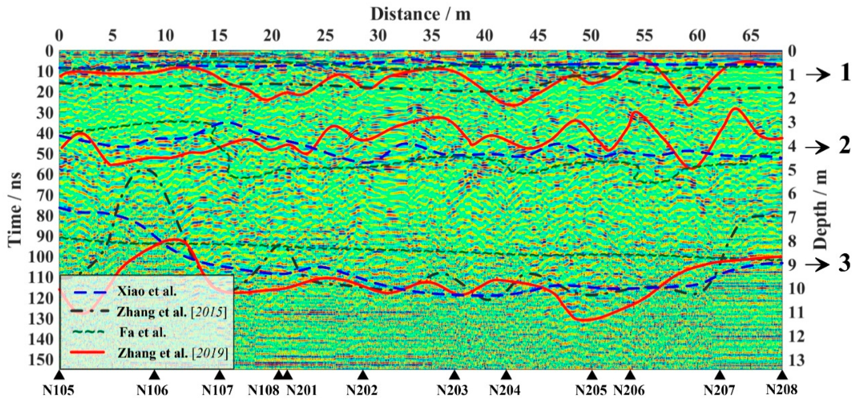
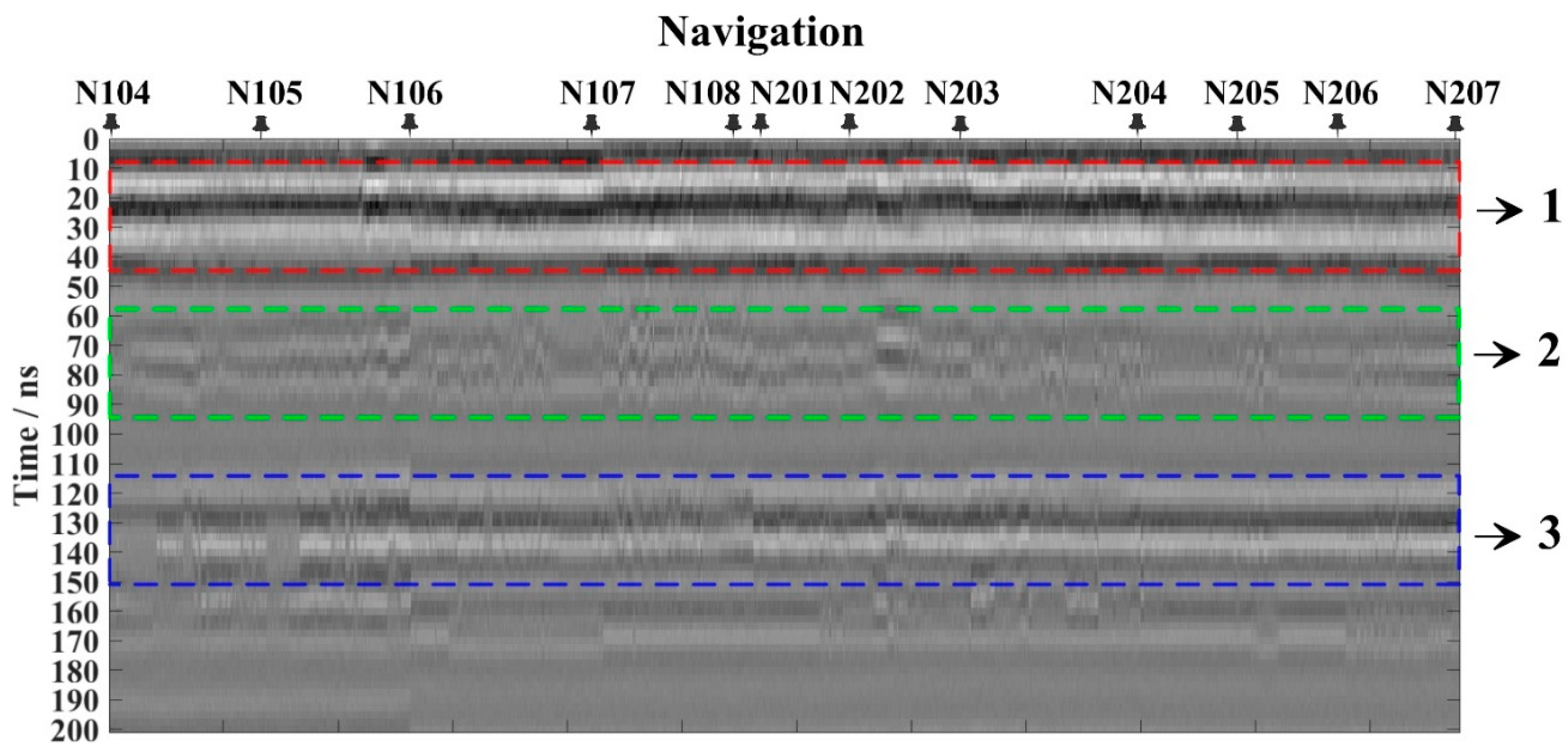
3.3. Data Interpretation

As can be known from the above analysis, only the frequencies of the IMF2 and IMF3 components are in accordance with the radar’s transmission frequency and are available. These two components are superimposed for further analytical interpretation. Figure 12a shows the data after IMF3 is superimposed with IMF4, and Figure 12b plots all the traces. From these two figures, especially in Figure 12b, it is found that the SNR of the data below 3000 ns is very low, making it difficult to pick up effective and convincing events. Therefore, we will focus on the shallow part.
Figure 13 shows the information within the shallow part of 3000 ns, but the events below 300 ns are not continuous. It is necessary to be very careful to interpret such information. This paper aims to decompose and analyze the CH-1 data, and the deep information no longer needs deeper explanation. Instead, information within the first 200 ns corresponding to the CH-2 data is selected for analysis. According to the hierarchical information of Xiao et al. [6], Zhang et al. [10], Fa et al. [11], and Zhang et al. [14], there are three well-recognized interfaces (Figure 14), namely:
  • The interface between the ejected materials of the Chang’E-3 crater and the lunar regolith;
  • The interface between the lunar regolith and paleoregolith;
  • The bedrock interface.
Figure 15 shows the information within 200 ns of the CH-1 data. There are three distinct events at the same position corresponding to the CH-2 data. It proves the rationality of stratification at the shallow part.

4. Discussion

In the use of CEEMD to process radar data, Li et al. used the CEEMD decomposition method not only to perform time–frequency analysis but also to perform denoising and target recognition on GPR data [26,27]. They mainly used CEEMD to decompose GPR data, used the Hilbert transform to analyze the data, and then performed denoising accordingly. The method in this paper not only uses CEEMD to decompose the data, but also uses the STFT and Hilbert transform to analyze the single component and the overall data comprehensively, which improves the application of CEEMD in ground-penetrating-radar processing.
On the other hand, regarding the use of CH-1 data from the lunar radar, although Li et al. [20] believed that Xiao et al. [6] and Zhang et al. [10] had objections to the use of CH-1 data, and used the ground experimental data and S transform to support their view, they did not perform in-depth decomposition and analysis of the overall CH-1 data. In this paper, the non-linear decomposition method is used to deeply analyze the false reflectors and available information of CH-1 data.
The most important significance of this paper is that the LPR data of CE-4 is being collected on the moon, and the CH-1 data collected by CE-4 can be used by the CEEMD combined with the short-time Fourier transform and the Hilbert in the case of an extremely low SNR. The idea of special transformation is analyzed to improve the credibility of the CE-4 data.

5. Conclusions

The LPR equipped on the YR measured the lunar geological structure in Northern Imbrium. As the data were complicated, a group of data preprocessing was designed. When the data were still distinct after preprocessing, the frequency spectrum and time–frequency spectrum of LPR CH-1 data were carried out for analysis. Subsequently, CEEMD helped to analyze the data, and the IMFs indicated the information distribution. Finally, combining with the previous studies and LPR CH-2 data, we proved the credibility of the CH-1 data at the shallow part.
CEEMD has been put forward as an adaptive time–frequency LPR data analysis method. It has been verified as quite multifunctional in extracting signals. The IMFs of the overall CH-1 data and the stagnation points’ traces describe the frequency information distribution. After comprehensively observing the CEEMD components of the overall CH-1 data and the CEEMD components of the stagnation points’ traces, it can be found that in IMF5, two pitfalls at 3500 and 5800 ns can be found. Only the frequencies of the IMF2 and IMF3 components are in accordance with the radar’s transmission frequency and are available. These two components are superimposed for further analytical interpretation. Superimposed components provide us with the chance to analyze geological information at the shallow part.
This paper aims to decompose and analyze the CH-1 data, and the deep information no longer needs a deeper explanation. Instead, information within the first 200 ns corresponding to the CH-2 data is selected for analysis. According to the hierarchical information of former researchers, there are three well-recognized interfaces. As the CE-4 LPR data are going to be published soon, CEEMD, which can prove the availability of the data, provides solid help and support for the articles published on the CE-4 radar data.
Those results obtained in this paper provide valuable reference for understanding LPR data and valuable information for future lunar exploration missions.

Author Contributions

Conceptualization, investigation and Writing, C.X.; Supervision, G.Z.; Formal analysis, Investigation, J.Z.; Formal analysis, Methodology, Z.J. All authors have read and agreed to the published version of the manuscript.

Funding

This research was supported by the Major Projects of the National Science and Technology of China (2016YFC0600505) and the National Natural Science Foundation of China under Grant 41574097 and 41504083.

Conflicts of Interest

The authors declare no conflict of interest.

Abbreviations

LPRLunar Penetrating Radar
CE-3Chang’E-3
CE-4Chang’E-4
CH-1The low-frequency channel
CH-2The high-frequency channel
HFhigh-frequency
CEEMDComplete Ensemble Empirical Mode Decomposition
DFRdual-frequency radar on the rover
SARsynthetic aperture radar
LRSLunar-Radar Sounder
SELENEJapan’s Kaguya probes
LROLunar-Reconnaissance-Orbiter
YRYutu rover
NAOCNational Astronomical Observatory of the Chinese Academy of Sciences
EMDEmpirical-Mode-Decomposition
IMFintrinsic mode function
EEMFEnsemble Empirical-Mode-Decomposition
NADAnew method of noise assisted data analysis
SNRSignal-to-noise ratio
FDfrequency-domain
TFDtime–frequency domain
FTFourier transform
STFTshort-time Fourier transform
VMDVariational Mode Decomposition

References

  1. Phillips, R.J.; Adams, G.F.; Brown, W.E., Jr.; Eggleton, R.E.; Zelenka, J.S. Apollo Lunar Sounder Experiment. Apollo 17 Prelim. Sci. Rep. 1973, 330, 22. [Google Scholar]
  2. Ono, T.; Kumamoto, A.; Nakagawa, H.; Yamaguchi, Y.; Oshigami, S.; Yamaji, A.; Kobayashi, T.; Kasahara, Y.; Oya, H. Lunar radar sounder observations of subsurface layers under the nearside maria of the moon. Science 2009, 323, 909–912. [Google Scholar] [CrossRef] [Green Version]
  3. Spudis, P.D.; Bussey, B.; Lichtenberg, C.; Marinelli, B.; Nozette, S. Mini-sar: An imaging radar for the chandrayaan-1 mission to the moon. Curr. Sci. 2005, 96, 533–539. [Google Scholar]
  4. Calla, O.P.N.; Mathur, S.; Jangid, M.; Gadri, K.L. Circular polarization characteristics of south polar lunar craters using chandrayaan-1 mini-sar and lro mini-rf. Earth Moon Planets 2015, 115, 83–100. [Google Scholar] [CrossRef]
  5. Patterson, G.W.; Stickle, A.M.; Turner, F.S.; Jensen, J.R.; Jakowatz, C.V. Bistatic radar observations of the moon using mini-rf on lro and the arecibo observatory. Icarus 2016, 283, 2–19. [Google Scholar] [CrossRef]
  6. Xiao, L.; Zhu, P.; Fang, G.; Xiao, Z.; Zou, Y.; Zhao, J.; Zhao, N.; Yuan, Y.; Qiao, L.; Zhang, X.; et al. A young multilayered terrane of the northern mare imbrium revealed by chang’e-3 mission. Science 2015, 347, 1226–1229. [Google Scholar] [CrossRef] [PubMed]
  7. Fang, G.-Y.; Zhou, B.; Ji, Y.-C.; Zhang, Q.-Y.; Shen, S.-X.; Li, Y.-X.; Guan, H.F.; Tang, C.J.; Gao, Y.Z.; Lu, W.; et al. Lunar penetrating radar onboard the chang’e-3 mission. Res. Astron. Astrophys. 2014, 14, 1607–1622. [Google Scholar] [CrossRef]
  8. Wilhelms, D.E.; Mccauley, J.F.; Trask, N.J. The Geologic History of the Moon; United States Government Publishing Office: Washington, DC, USA, 1987.
  9. Su, Y.; Fang, G.-Y.; Feng, J.-Q.; Xing, S.-G.; Ji, Y.-C.; Zhou, B.; Gao, Y.Z.; Li, H.; Dai, S.; Xiao, Y.; et al. Data processing and initial results of Chang’e-3 lunar penetrating radar. Res. Astron. Astrophys. 2014, 14, 1623–1632. [Google Scholar] [CrossRef]
  10. Zhang, J.; Yang, W.; Hu, S.; Lin, Y.; Fang, G.; Li, C.; Peng, W.; Zhu, S.; He, Z.; Zhou, B. Volcanic history of the imbrium basin: A close-up view from the lunar rover yutu. Proc. Natl. Acad. Sci. USA 2015, 112, 5342–5347. [Google Scholar] [CrossRef] [Green Version]
  11. Fa, W.; Zhu, M.H.; Liu, T.; Plescia, J.B. Regolith stratigraphy at the chang’e-3 landing site as seen by lunar penetrating radar. Geophys. Res. Lett. 2015, 42, 179–187. [Google Scholar] [CrossRef]
  12. Lai, J.L.; Xu, Y.; Zhang, X.P.; Tang, Z.S. Structural analysis of lunar subsurface with Chang'E-3 lunar penetrating radar. Planet. Space Sci. 2016, 120, 96–102. [Google Scholar] [CrossRef]
  13. Zhang, L.; Zeng, Z.; Li, J.; Lin, J.; Hu, Y.; Wang, X.; Sun, X. Simulation of the lunar regolith and lunar-penetrating radar data processing. IEEE J. Sel. Top. Appl. Earth Obs. Remote. Sens. 2018, 11, 655–663. [Google Scholar] [CrossRef]
  14. Zhang, L.; Zeng, Z.F.; Li, J.; Huang, L.; Huo, Z.J.; Wang, K.; Zhang, J.M. A Story of Regolith Told by Lunar Penetrating Radar. Icarus 2019, 321, 148–160. [Google Scholar] [CrossRef]
  15. Dong, Z.; Fang, G.; Ji, Y.; Gao, Y.; Zhang, X. Parameters and structure of lunar regolith in chang’e-3 landing area from lunar penetrating radar (lpr) data. Icarus 2016, 282, 40–46. [Google Scholar] [CrossRef]
  16. Zhang, L.; Zeng, Z.; Li, J.; Huang, L.; Huo, Z.; Wang, K.; Zhang, J. Parameter Estimation of Lunar Regolith from Lunar Penetrating Radar Data. Sensors 2018, 18, 2907. [Google Scholar] [CrossRef] [Green Version]
  17. Wang, K.; Zeng, Z.; Zhang, L.; Xia, S.; Li, J. A Compressive Sensing-Based Approach to Reconstructing Regolith Structure from Lunar Penetrating Radar Data at the Chang’E-3 Landing Site. Remote Sens. 2018, 10, 1925. [Google Scholar] [CrossRef] [Green Version]
  18. Zhang, J.; Zeng, Z.; Zhang, L.; Lu, Q.; Wang, K. Application of Mathematical Morphological Filtering to Improve the Resolution of Chang’e-3 Lunar Penetrating Radar Data. Remote Sens. 2019, 11, 524. [Google Scholar] [CrossRef] [Green Version]
  19. Hu, B.; Wang, D.; Zhang, L.; Zeng, Z. Rock Location and Quantitative Analysis for Regolith on Chang’e 3 Landing Site Based on Local Similarity Constraint. Remote Sens. 2019, 11, 530. [Google Scholar] [CrossRef] [Green Version]
  20. Li, C.; Xing, S.; Lauro, S.E.; Su, Y.; Pettinelli, E. Pitfalls in gpr data interpretation: False reflectors detected in lunar radar cross sections by chang’e-3. IEEE Trans. Geosci. Remote Sens. 2017, 56, 1325–1335. [Google Scholar] [CrossRef]
  21. Huang, N.E.; Shen, Z.; Long, S.R.; Wu, M.C.; Shih, H.H.; Zheng, Q.; Yen, N.C.; Tung, C.C.; Liu, H.H. The empirical mode decomposition and the hilbert spectrum for nonlinear and non-stationary time series analysis. Proc. R. Soc. London Ser. A 1998, 454, 903–995. [Google Scholar] [CrossRef]
  22. Wu, Z.; Huang, N.E. Ensemble empirical mode decomposition: A noise-assisted data analysis method. Adv. Adapt. Data Anal. 2009, 1, 1–41. [Google Scholar] [CrossRef]
  23. Torres, M.E.; Colominas, M.A.; Schlotthauer, G.; Flandrin, P. A complete ensemble empirical mode decomposition with adaptive noise. In Proceedings of the IEEE International Conference on Acoustics, Speech and Signal, Prague, Czech Republic, 22–27 May 2011; pp. 22–27. [Google Scholar]
  24. Jia, Z.; Liu, S.; Zhang, L.; Hu, B.; Zhang, J. Weak Signal Extraction from Lunar Penetrating Radar Channel 1 Data Based on Local Correlation. Electronics 2019, 8, 573. [Google Scholar] [CrossRef] [Green Version]
  25. Cheng, S.; Liu, S.; Guo, J.; Luo, K.; Zhang, L.; Tang, X. Data Processing and Interpretation of Antarctic Ice-Penetrating Radar Based on Variational Mode Decomposition. Remote Sens. 2019, 11, 1253. [Google Scholar] [CrossRef] [Green Version]
  26. Li, J.; Liu, C.; Zeng, Z.; Chen, L. GPR Signal Denoising and Target Extraction with the CEEMD Method. IEEE Geosci. Remote Sens. Lett. 2015, 12, 1615–1619. [Google Scholar]
  27. Li, J.; Zeng, Z.; Liu, C.; Huai, N.; Wang, K. A study on Lunar regolith quantitative random model and lunar penetrating radar parameter inversion. IEEE Geosci. Remote Sens. Lett. 2017, 14, 1953–1957. [Google Scholar] [CrossRef]
Figure 1. Walking track of Yutu. This picture has come from the descent camera on the Chang’E-3 (CE-3) lander.
Applsci 10 00535 g001
Figure 2. Lunar Penetrating Radar (LPR) CH-1 data from N104 to N207 after preprocessing. (a) All traces from N104 to N207. (b) The traces after deleting the repeated traces. (c) The stagnation traces at each recording and navigation point from N104 to N207.
Applsci 10 00535 g002
Figure 3. The decomposition flowchart of empirical mode decomposition (EMD).
Applsci 10 00535 g003
Figure 4. Frequency spectrum of traces. (a) N104. (b) N106. (c) N202. (d) N206.
Applsci 10 00535 g004
Figure 5. Time–frequency spectrum of (a) N104, (b) N106, (c) N202, and (d) N206 traces.
Applsci 10 00535 g005
Figure 6. (a) LPR CH-1 overall data and (b) stagnation points’ traces after gain.
Applsci 10 00535 g006
Figure 7. Analysis of the trace at N104 by complete ensemble empirical mode decomposition (CEEMD).
Applsci 10 00535 g007
Figure 8. Time–frequency spectrum of each intrinsic mode function (IMF) decomposed from the trace at N104. (a) IMF1. (b) IMF2. (c) IMF3. (d) IMF4. (e) IMF5. (f) IMF6. (g) IMF7. (h) Residual.
Applsci 10 00535 g008
Figure 9. Hilbert spectrum of IMFs from N104.
Applsci 10 00535 g009
Figure 10. IMFs of LPR CH-1 overall data. (a) IMF1. (b) IMF2. (c) IMF3. (d) IMF4. (e) IMF5. (f) IMF6. (g) IMF7. (h) Residual.
Applsci 10 00535 g010
Figure 11. IMFs of stagnation points’ traces in Figure 7. (a) IMF1. (b) IMF2. (c) IMF3. (d) IMF4. (e) IMF5. (f) IMF6. (g) IMF7. (h) Residual.
Applsci 10 00535 g011
Figure 12. (a) Superimposed component of IMF3 and IMF4 and (b) all the traces.
Applsci 10 00535 g012
Figure 13. Superimposed component of IMF3 and IMF4. (a) 0–1000, (b) 1000–2000, and (c) 2000–3000 ns.
Applsci 10 00535 g013
Figure 14. Stratification on CE-3 landing site by CH-2 data.
Applsci 10 00535 g014
Figure 15. Stratification on CE-3 landing site by CH-1 data.
Applsci 10 00535 g015
Table 1. Data preprocessing instructions.
ProcessingInterpretative Statement
iData readingThe data is decomposed into 9 parts. According to their storage format (*.psd, which is the standard storage format for aerospace and aerospace), data and location information will be read one by one.
iiData registrationThe data is split into 9 parts and ought to be stitched together.
iiiTime lag adjustmentThe arrival time of the radar echo is delayed by 69.664 ns, which corresponds to the start time of the recorded data.
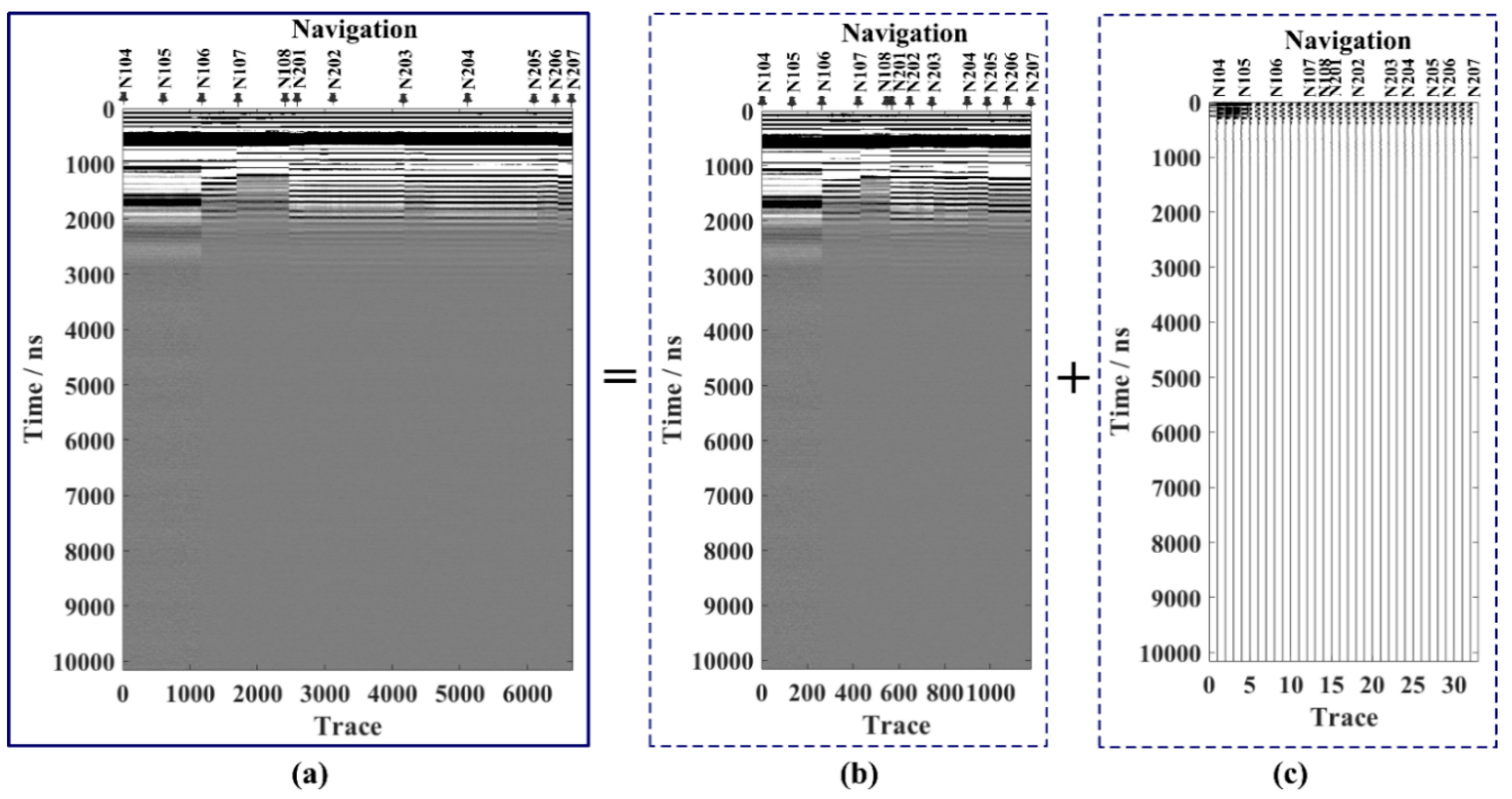
ivDeep useless data deletingAs the SNRs of Part 1 and Part 2 are low and the rest of the data are not collected, the last 10,000 ns of data without the study value needs to be deleted.
vLow SNR traces deletingSome parts with low SNR should be removed.
viTraces selectingRover patrols are uneven because the rover may stop at a waypoint to collect other scientific data, for example, APXS data, VNIS data, and so forth. However, LPR never stops collecting data, which results in multiple acquisitions of multiple traces at the same place. The repeating traces are stacked and averaged. Two sets of data are obtained. One is all data without a copy track, and the other is a repeating track that has been stacked and averaged at the waypoint.
viiLocationLocation information is added to the image.

