An Efficient Algorithm for Cardiac Arrhythmia Classification Using Ensemble of Depthwise Separable Convolutional Neural Networks


Abstract
1. Introduction
2. 1D Convolutional Neural Network and Its Enhancement
2.1. 1-D CNNs
2.2. All Convolutional Network
2.3. Batch Normalization
2.4. Depthwise Separable Convolution
3. Proposed Ensemble of Depthwise Separable Convolutional Neural Networks
3.1. Beat Detection and Segmentation
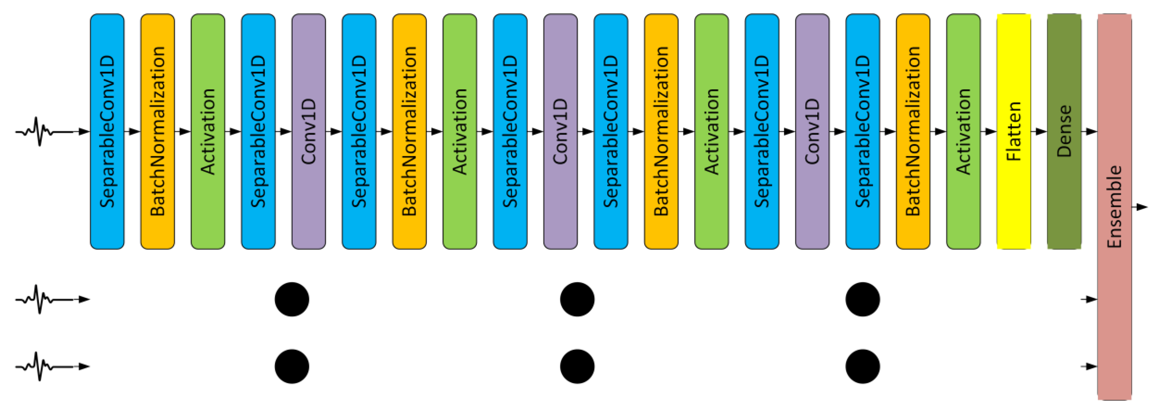
3.2. Ensemble CNNs
4. Implementation and Experimental Setup
4.1. MIT-BIH Arrhythmia Database and Computing Platform
4.2. Depthwise Separable and Ensemble of Depthwise Separable CNN Models
5. Results and Discussion
5.1. Experiment on ECG Beat Segmentation and Detection
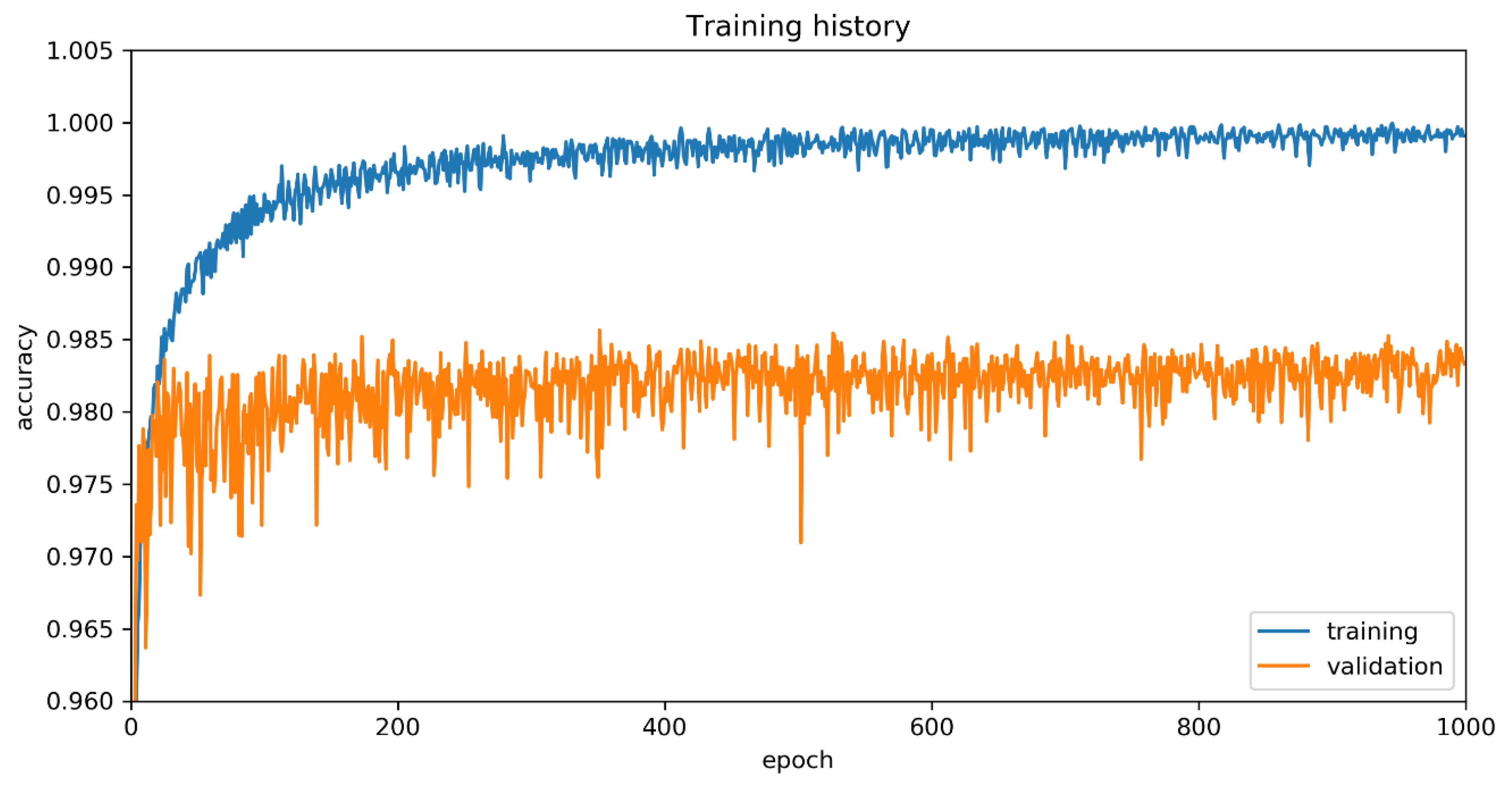
5.2. Training Process
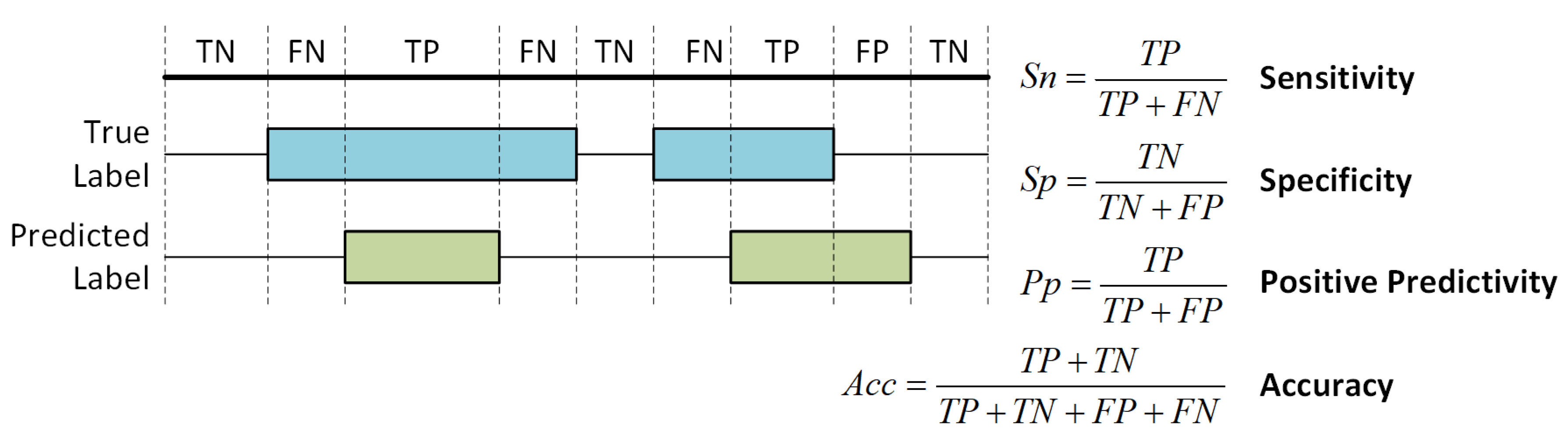
5.3. Performance Measures
5.4. On the Effect of Depthwise Separable CNN
5.5. On the Effect of Zero Padding
5.6. On the Effect of Various Ensemble Configurations
5.7. On Comparison with Other Algorithms
6. Conclusions
Author Contributions
Funding
Conflicts of Interest
References
- Evans, G.F.; Shirk, A.; Muturi, P.; Soliman, E.Z. Feasibility of using mobile ECG recording technology to detect atrial fibrillation in low-resource settings. Glob. Heart 2017, 12, 285–289. [Google Scholar] [CrossRef] [PubMed]
- Sun, W.; Zeng, N.; He, Y. Morphological Arrhythmia Automated Diagnosis Method Using Gray-Level Co-occurrence Matrix Enhanced Convolutional Neural Network. IEEE Access 2019, 7, 67123–67129. [Google Scholar] [CrossRef]
- Laguna, P.; Cortés, J.P.M.; Pueyo, E. Techniques for ventricular repolarization instability assessment from the ECG. Proc. IEEE 2016, 104, 392–415. [Google Scholar] [CrossRef]
- Satija, U.; Ramkumar, B.; Manikandan, M.S. A New Automated Signal Quality-Aware ECG Beat Classification Method for Unsupervised ECG Diagnosis Environments. IEEE Sens. J. 2018, 19, 277–286. [Google Scholar] [CrossRef]
- Lynn, H.M.; Pan, S.B.; Kim, P. A Deep Bidirectional GRU Network Model for Biometric Electrocardiogram Classification Based on Recurrent Neural Networks. IEEE Access 2019, 7, 145395–145405. [Google Scholar] [CrossRef]
- Chu, Y.; Shen, H.; Huang, K. ECG Authentication Method Based on Parallel Multi-Scale One-Dimensional Residual Network With Center and Margin Loss. IEEE Access 2019, 7, 51598–51607. [Google Scholar] [CrossRef]
- Kim, H.; Chun, S.Y. Cancelable ECG Biometrics Using Compressive Sensing-Generalized Likelihood Ratio Test. IEEE Access 2019, 7, 9232–9242. [Google Scholar] [CrossRef]
- Dokur, Z.; Olmez, T.; Yazgan, E. Comparison of discrete wavelet and Fourier transforms for ECG beat classification. Electron. Lett. 1999, 35, 1502–1504. [Google Scholar] [CrossRef]
- Banerjee, S.; Mitra, M. Application of cross wavelet transform for ECG pattern analysis and classification. IEEE Trans. Instrum. Meas. 2013, 63, 326–333. [Google Scholar] [CrossRef]
- Melgani, F.; Bazi, Y. Classification of electrocardiogram signals with support vector machines and particle swarm optimization. IEEE Trans. Inf. Technol. Biomed. 2008, 12, 667–677. [Google Scholar] [CrossRef]
- Venkatesan, C.; Karthigaikumar, P.; Paul, A.; Satheeskumaran, S.; Kumar, R. ECG signal preprocessing and SVM classifier-based abnormality detection in remote healthcare applications. IEEE Access 2018, 6, 9767–9773. [Google Scholar] [CrossRef]
- Chen, X.; Wang, Y.; Wang, L. Arrhythmia Recognition and Classification Using ECG Morphology and Segment Feature Analysis. IEEE/ACM Trans. Comput. Biol. Bioinform. 2018, 16, 131–138. [Google Scholar]
- Raj, S.; Ray, K.C. ECG signal analysis using DCT-based DOST and PSO optimized SVM. IEEE Trans. Instrum. Meas. 2017, 66, 470–478. [Google Scholar] [CrossRef]
- Pasolli, E.; Melgani, F. Active learning methods for electrocardiographic signal classification. IEEE Trans. Inf. Technol. Biomed. 2010, 14, 1405–1416. [Google Scholar] [CrossRef]
- Li, Z.; Feng, X.; Wu, Z.; Yang, C.; Bai, B.; Yang, Q. Classification of Atrial Fibrillation Recurrence Based on a Convolution Neural Network With SVM Architecture. IEEE Access 2019, 7, 77849–77856. [Google Scholar] [CrossRef]
- Zigel, Y.; Cohen, A.; Katz, A. The weighted diagnostic distortion (WDD) measure for ECG signal compression. IEEE Trans. Biomed. Eng. 2000, 47, 1422–1430. [Google Scholar]
- Gerencsér, L.; Kozmann, G.; Vago, Z.; Haraszti, K. The use of the SPSA method in ECG analysis. IEEE Trans. Biomed. Eng. 2002, 49, 1094–1101. [Google Scholar] [CrossRef]
- Rahman, Q.A.; Tereshchenko, L.G.; Kongkatong, M.; Abraham, T.; Abraham, M.R.; Shatkay, H. Utilizing ECG-based heartbeat classification for hypertrophic cardiomyopathy identification. IEEE Trans. Nanobiosci. 2015, 14, 505–512. [Google Scholar] [CrossRef]
- Sopic, D.; Aminifar, A.; Aminifar, A.; Atienza, D. Real-time event-driven classification technique for early detection and prevention of myocardial infarction on wearable systems. IEEE Trans. Biomed. Circuits Syst. 2018, 12, 982–992. [Google Scholar] [CrossRef]
- Lai, D.; Zhang, Y.; Zhang, X. An automated strategy for early risk identification of sudden cardiac death by using machine learning approach on measurable arrhythmic risk markers. IEEE Access 2019, 7, 94701–94716. [Google Scholar] [CrossRef]
- Rad, A.B.; Eftestol, T.; Engan, K.; Irusta, U.; Kvaloy, J.T.; Kramer-Johansen, J.; Wik, L.; Katsaggelos, A.K. ECG-based classification of resuscitation cardiac rhythms for retrospective data analysis. IEEE Trans. Biomed. Eng. 2017, 64, 2411–2418. [Google Scholar] [CrossRef] [PubMed]
- Fira, C.M.; Goras, L. An ECG signals compression method and its validation using NNs. IEEE Trans. Biomed. Eng. 2008, 55, 1319–1326. [Google Scholar] [CrossRef] [PubMed]
- Mar, T.; Zaunseder, S.; Martínez, J.P.; Llamedo, M.; Poll, R. Optimization of ECG classification by means of feature selection. IEEE Trans. Biomed. Eng. 2011, 58, 2168–2177. [Google Scholar] [CrossRef]
- Bouaziz, F.; Oulhadj, H.; Boutana, D.; Siarry, P. Automatic ECG arrhythmias classification scheme based on the conjoint use of the multi-layer perceptron neural network and a new improved metaheuristic approach. IET Signal Process. 2019, 13, 726–735. [Google Scholar] [CrossRef]
- Huang, J.; Chen, B.; Yao, B.; He, B. ECG arrhythmia classification using STFT-based spectrogram and convolutional neural network. IEEE Access 2019, 7, 92871–92880. [Google Scholar] [CrossRef]
- Mai, V.; Khalil, I.; Meli, C. ECG biometric using multilayer perceptron and radial basis function neural networks. In Proceedings of the 2011 Annual International Conference of the IEEE Engineering in Medicine and Biology Society, Boston, MA, USA, 30 August–3 September 2011. [Google Scholar]
- Kiranyaz, S.; Ince, T.; Gabbouj, M. Real-time patient-specific ECG classification by 1-D convolutional neural networks. IEEE Trans. Biomed. Eng. 2015, 63, 664–675. [Google Scholar] [CrossRef]
- Nurmaini, S.; Partan, R.U.; Caesarendra, W.; Dewi, T.; Rahmatullah, M.N.; Darmawahyuni, A.; Bhayyu, V.; Firdaus, F. An Automated ECG Beat Classification System Using Deep Neural Networks with an Unsupervised Feature Extraction Technique. Appl. Sci. 2019, 9, 2921. [Google Scholar] [CrossRef]
- Zhai, X.; Tin, C. Automated ECG classification using dual heartbeat coupling based on convolutional neural network. IEEE Access 2018, 6, 27465–27472. [Google Scholar] [CrossRef]
- Springenberg, J.T.; Dosovitskiy, A.; Brox, T.; Riedmiller, M. Striving for simplicity: The all convolutional net. arXiv 2014, arXiv:1412.6806. [Google Scholar]
- Ioffe, S.; Szegedy, C. Batch normalization: Accelerating deep network training by reducing internal covariate shift. arXiv 2015, arXiv:1502.03167. [Google Scholar]
- Kaiser, L.; Gomez, A.N.; Chollet, F. Depthwise separable convolutions for neural machine translation. arXiv 2017, arXiv:1706.03059,. [Google Scholar]
- Polikar, R. Ensemble learning. In Ensemble Machine Learning; Springer: Berlin, Germany, 2012; pp. 1–34. [Google Scholar]
- Chollet, F. Xception: Deep learning with depthwise separable convolutions. In Proceedings of the IEEE Conference on Computer Vision and Pattern Recognition, Honolulu, HI, USA, 21–26 July 2017. [Google Scholar]
- Zhang, T.; Zhang, X.; Shi, J.; Wei, S. Depthwise Separable Convolution Neural Network for High-Speed SAR Ship Detection. Remote Sens. 2019, 11, 2483. [Google Scholar] [CrossRef]
- Ince, T.; Kiranyaz, S.; Gabbouj, M. A generic and robust system for automated patient-specific classification of ECG signals. IEEE Trans. Biomed. Eng. 2009, 56, 1415–1426. [Google Scholar] [CrossRef] [PubMed]
- Wen, C.; Lib, T.-C.; Chang, K.-C.; Huang, C.-H. Classification of ECG complexes using self-organizing CMAC. Measurement 2009, 42, 399–407. [Google Scholar] [CrossRef]
- Rajpurkar, P.; Hannun, A.Y.; Rajpurkar, P.; Haghpanahi, M.; Tison, G.H.; Bourn, C.; Turakhia, M.P.; Ng, A.Y. Cardiologist-level arrhythmia detection with convolutional neural networks. arXiv 2017, arXiv:1707.01836. [Google Scholar]
- Pan, J.; Tompkins, W.J. A real-time QRS detection algorithm. IEEE Trans. Biomed. Eng. 1985, 32, 230–236. [Google Scholar] [CrossRef]
- Li, C.; Zheng, C.; Tai, C. Detection of ECG characteristic points using wavelet transforms. IEEE Trans. Biomed. Eng. 1995, 42, 21–28. [Google Scholar]
- Moody, G.B.; Mark, A.R.G. The impact of the MIT-BIH arrhythmia database. IEEE Eng. Med. Biol. Mag. 2001, 20, 45–50. [Google Scholar] [CrossRef]
- Dupre, A.; Vincent, S.; Iaizzo, P.A. Basic ECG Theory, Recordings, and Interpretation. In Handbook of Cardiac Anatomy, Physiology, and Devices; Springer: Berlin, Germany, 2005; pp. 191–201. [Google Scholar]
- Abadi, M.; Barham, P.; Chen, J.; Chen, Z.; Davis, A.; Dean, J.; Devin, M.; Ghemawat, S.; Irving, G.; Isard, M.; et al. Tensorflow: A system for large-scale machine learning. In Proceedings of the 12th USENIX Symposium on Operating Systems Design and Implementation (OSDI16), Savannah, GA, USA, 2–4 November 2016. [Google Scholar]
- Chollet, F. Keras: Deep Learning Library for Theano and Tensorflow. 2015. Available online: https://keras.io/ (accessed on 20 May 2019).
- Hu, Y.H.; Palreddy, S.; Tompkins, W.J. A patient-adaptable ECG beat classifier using a mixture of experts approach. IEEE Trans. Biomed. Eng. 1997, 44, 891–900. [Google Scholar]
- Sarfraz, M.; Khan, A.A.; Li, F.F. Using independent component analysis to obtain feature space for reliable ECG Arrhythmia classification. In Proceedings of the 2014 IEEE International Conference on Bioinformatics and Biomedicine (BIBM), Belfast, UK, 2–5 November 2014. [Google Scholar]
- Xia, Y.; Zhang, H.; Xu, L.; Gao, Z.; Zhang, H.; Liu, H.; Li, S. An automatic cardiac arrhythmia classification system with wearable electrocardiogram. IEEE Access 2018, 6, 16529–16538. [Google Scholar] [CrossRef]
- Nanjundegowda, R.; Meshram, V.A. Arrhythmia Detection Based on Hybrid Features of T-wave in Electrocardiogram. Int. J. Intell. Eng. Syst. 2018, 11, 153–162. [Google Scholar] [CrossRef]
- Rangappa, V.G.; Prasad, S.V.A.V.; Agarwal, A. Classification of Cardiac Arrhythmia stages using Hybrid Features Extraction with K-Nearest Neighbour classifier of ECG Signals. Learning 2018, 11, 21–32. [Google Scholar]


| No | Symbol | Annotation Description | Total | Training | Testing |
|---|---|---|---|---|---|
| 1 | N | Normal beat | 75,052 | 11,257 | 63,795 |
| 2 | L | Left bundle branch block beat | 8075 | 2826 | 5249 |
| 3 | R | Right bundle branch block beat | 7259 | 2540 | 4719 |
| 4 | V | Premature ventricular contraction | 7130 | 2495 | 4635 |
| 5 | / | Paced beat | 7028 | 2459 | 4569 |
| 6 | A | Atrial premature contraction | 2546 | 891 | 1655 |
| 7 | f | Fusion of paced and normal beat | 982 | 491 | 491 |
| 8 | F | Fusion of ventricular and normal beat | 803 | 401 | 402 |
| 9 | ! | Ventricular flutter wave | 472 | 236 | 236 |
| 10 | j | Nodal (junctional) escape beat | 229 | 114 | 115 |
| 11 | x | Non-conducted P-wave | 193 | 96 | 97 |
| 12 | a | Aberrated atrial premature beat | 150 | 75 | 75 |
| 13 | E | Ventricular escape beat | 106 | 53 | 53 |
| 14 | J | Nodal (junctional) premature beat | 83 | 41 | 42 |
| 15 | e | Atrial escape beat | 16 | 8 | 8 |
| 16 | Q | Unclassifiable beat | 33 | 16 | 17 |
| Total 16-class beats | 110,157 | 23,999 | 86,158 | ||
| Extracted from total 112,647 of labeled ECG beats | |||||
| # | Layer | Number of Filters, Size, Stride | Output Shape | Number of Parameters |
|---|---|---|---|---|
| 1 | input_1 | (256, 1) | 0 | |
| 2 | separable_conv1d_1 | 32, 5, 4 | (64, 32) | 69 |
| 3 | batch_normalization_1 | (64, 32) | 128 | |
| 4 | activation_1 | (64, 32) | 0 | |
| 5 | separable_conv1d_2 | 32, 5, 1 | (64, 32) | 1216 |
| 6 | conv1d_1 | 32, 1, 1 | (64, 32) | 1056 |
| 7 | separable_conv1d_3 | 32, 5, 4 | (16, 32) | 1216 |
| 8 | batch_normalization_2 | (16, 32) | 128 | |
| 9 | activation_2 | (16, 32) | 0 | |
| 10 | separable_conv1d_4 | 32, 5, 1 | (16, 32) | 1216 |
| 11 | conv1d_2 | 32, 1, 1 | (16, 32) | 1056 |
| 12 | separable_conv1d_5 | 32, 5, 4 | (4, 32) | 1216 |
| 13 | batch_normalization_3 | (4, 32) | 128 | |
| 14 | activation_3 | (4, 32) | 0 | |
| 15 | separable_conv1d_6 | 32, 5, 1 | (4, 32) | 1216 |
| 16 | conv1d_3 | 32, 1, 1 | (4, 32) | 1056 |
| 17 | separable_conv1d_7 | 32, 5, 4 | (1, 32) | 1216 |
| 18 | batch_normalization_4 | (1, 32) | 128 | |
| 19 | activation_4 | (1, 32) | 0 | |
| 20 | flatten_1 | (32) | 0 | |
| 21 | dense_1 (Dense) | (16) | 528 | |
| Total parameters: 11,573 Trainable parameters: 11,317 Non-trainable parameters: 256 | ||||
| # | DSC | Total Parameters | TN | FN | TP | FP | Training Time | Testing Time | ||||
|---|---|---|---|---|---|---|---|---|---|---|---|---|
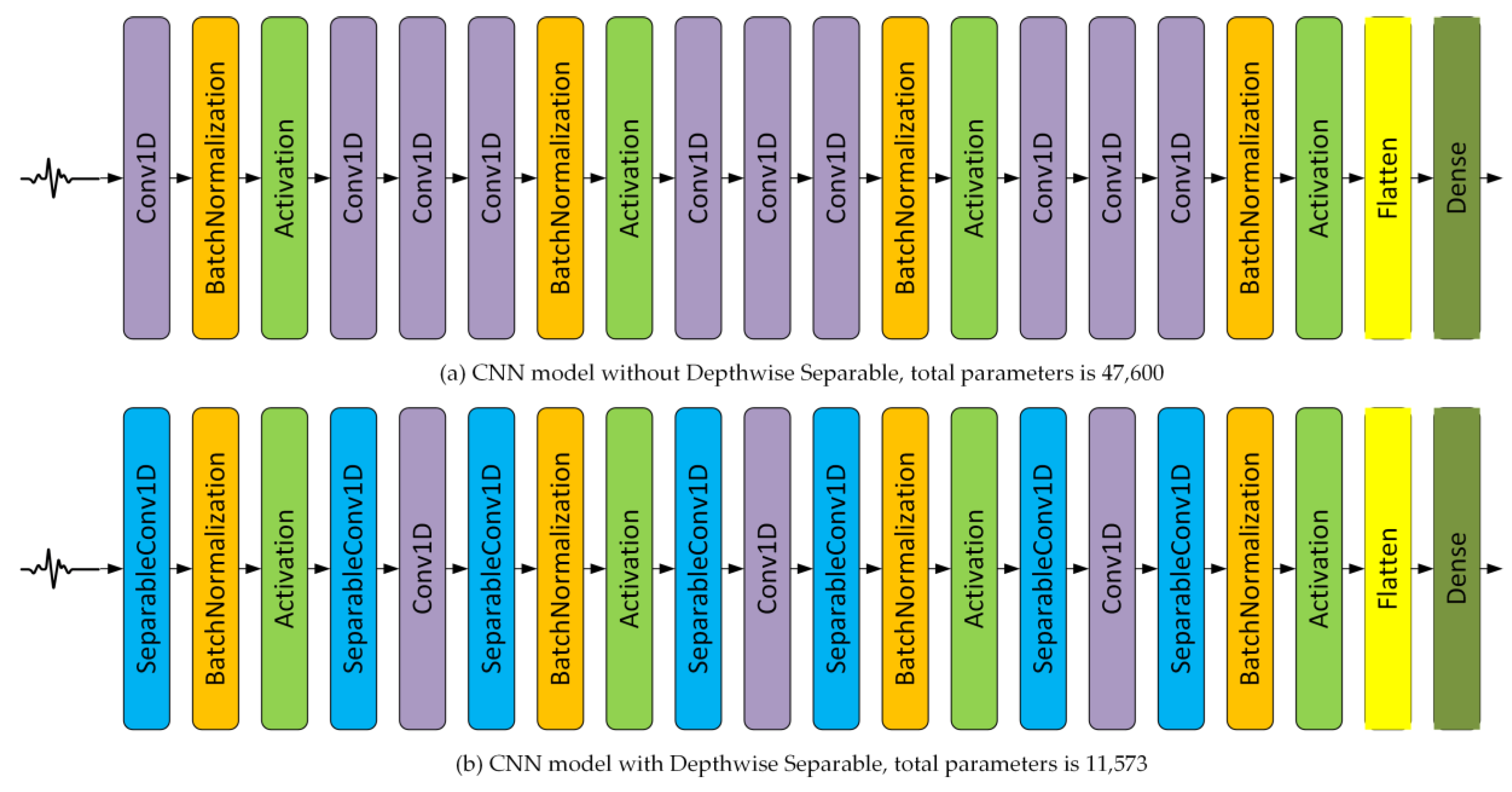
| 1 | Without DSC | 47,600 | 1,291,271 | 1099 | 85,059 | 1099 | 98.72 | 99.91 | 98.72 | 99.84 | 711.9 s | 81 s |
| 2 | With DSC | 11,573 | 1,290,966 | 1404 | 84,754 | 1404 | 98.37 | 99.89 | 98.37 | 99.80 | 745.8 s | 62 s |
| # | Zero Padding | Input Size | TN | FN | TP | FP | ||||
|---|---|---|---|---|---|---|---|---|---|---|
| 1 | No | 64 | 1,291,190 | 1180 | 84,978 | 1180 | 98.63 | 99.91 | 98.63 | 99.83 |
| 2 | No | 128 | 1,291,413 | 957 | 85,201 | 957 | 98.89 | 99.93 | 98.89 | 99.86 |
| 3 | No | 256 | 1,291,411 | 959 | 85,199 | 959 | 98.89 | 99.93 | 98.89 | 99.86 |
| 4 | Yes | 64 | 1,291,207 | 1163 | 84,995 | 1163 | 98.65 | 99.91 | 98.65 | 99.83 |
| 5 | Yes | 128 | 1,291,389 | 981 | 85,177 | 981 | 98.86 | 99.92 | 98.86 | 99.86 |
| 6 | Yes | 256 | 1,291,531 | 839 | 85,319 | 839 | 99.03 | 99.94 | 99.03 | 99.88 |
| # | Ensemble Configuration | TN | FN | TP | FP | Testing Time | ||||
|---|---|---|---|---|---|---|---|---|---|---|
| 1 | [128 64] | 1,291,194 | 1176 | 84,982 | 1176 | 98.64 | 99.91 | 98.64 | 99.83 | 111 s |
| 2 | [256 128] | 1,291,369 | 1001 | 85,157 | 1001 | 98.84 | 99.92 | 98.84 | 99.85 | 113 s |
| 3 | [256 256] | 1,291,460 | 910 | 85,248 | 910 | 98.94 | 99.93 | 98.94 | 99.87 | 111 s |
| 4 | [64 64 64] | 1,291,207 | 1163 | 84,995 | 1163 | 98.65 | 99.91 | 98.65 | 99.83 | 143 s |
| 5 | [128 128 128] | 1,291,389 | 981 | 85,177 | 981 | 98.86 | 99.92 | 98.86 | 99.86 | 146 s |
| 6 | [256 256 256] | 1,291,531 | 839 | 85,319 | 839 | 99.03 | 99.94 | 99.03 | 99.88 | 150 s |
| 7 | [256 128 64] | 1,291,408 | 962 | 85,196 | 962 | 98.88 | 99.93 | 98.88 | 99.86 | 150 s |
| Prediction | |||||||||||||||||
|---|---|---|---|---|---|---|---|---|---|---|---|---|---|---|---|---|---|
| N | L | R | V | / | A | f | F | ! | j | x | a | E | J | e | Q | ||
| Ground Truth | 0 | 1 | 2 | 3 | 4 | 5 | 6 | 7 | 8 | 9 | 10 | 11 | 12 | 13 | 14 | 15 | |
| N | 0 | 63,521 | 4 | 13 | 70 | 2 | 79 | 11 | 36 | 3 | 44 | 6 | 2 | 0 | 1 | 0 | 3 |
| L | 1 | 22 | 5211 | 0 | 13 | 1 | 0 | 0 | 0 | 0 | 0 | 0 | 0 | 1 | 0 | 0 | 1 |
| R | 2 | 11 | 0 | 4699 | 0 | 0 | 9 | 0 | 0 | 0 | 0 | 0 | 0 | 0 | 0 | 0 | 0 |
| V | 3 | 46 | 10 | 0 | 4528 | 1 | 11 | 0 | 22 | 10 | 0 | 0 | 7 | 0 | 0 | 0 | 0 |
| / | 4 | 3 | 0 | 0 | 3 | 4553 | 0 | 9 | 0 | 0 | 0 | 0 | 0 | 1 | 0 | 0 | 0 |
| A | 5 | 143 | 0 | 5 | 16 | 0 | 1484 | 0 | 2 | 0 | 3 | 0 | 0 | 0 | 2 | 0 | 0 |
| f | 6 | 13 | 0 | 0 | 1 | 6 | 0 | 470 | 0 | 0 | 0 | 0 | 0 | 0 | 1 | 0 | 0 |
| F | 7 | 52 | 0 | 0 | 36 | 0 | 0 | 0 | 313 | 0 | 0 | 1 | 0 | 0 | 0 | 0 | 0 |
| ! | 8 | 2 | 0 | 0 | 8 | 0 | 0 | 0 | 0 | 225 | 0 | 0 | 1 | 0 | 0 | 0 | 0 |
| j | 9 | 15 | 0 | 1 | 0 | 0 | 0 | 0 | 0 | 0 | 97 | 0 | 0 | 0 | 2 | 0 | 0 |
| x | 10 | 1 | 0 | 0 | 1 | 0 | 0 | 0 | 0 | 5 | 0 | 89 | 1 | 0 | 0 | 0 | 0 |
| a | 11 | 6 | 0 | 0 | 15 | 0 | 9 | 0 | 0 | 1 | 0 | 0 | 44 | 0 | 0 | 0 | 0 |
| E | 12 | 2 | 0 | 0 | 1 | 0 | 0 | 0 | 0 | 0 | 0 | 0 | 0 | 50 | 0 | 0 | 0 |
| J | 13 | 7 | 0 | 0 | 0 | 0 | 3 | 0 | 0 | 0 | 0 | 0 | 0 | 0 | 32 | 0 | 0 |
| e | 14 | 3 | 0 | 0 | 0 | 0 | 1 | 1 | 0 | 0 | 0 | 0 | 0 | 0 | 0 | 3 | 0 |
| Q | 15 | 11 | 0 | 2 | 1 | 0 | 0 | 3 | 0 | 0 | 0 | 0 | 0 | 0 | 0 | 0 | 0 |
| ECG Class | Total Beats | Train Beats | Test Beats | TN | FN | TP | FP | Acc | |||
|---|---|---|---|---|---|---|---|---|---|---|---|
| N | 75,052 | 11,257 | 63,795 | 22,026 | 274 | 63,521 | 337 | 99.57 | 98.49 | 99.47 | 99.29 |
| L | 8075 | 2826 | 5249 | 80,895 | 38 | 5211 | 14 | 99.28 | 99.98 | 99.73 | 99.94 |
| R | 7259 | 2540 | 4719 | 81,418 | 20 | 4699 | 21 | 99.58 | 99.97 | 99.56 | 99.95 |
| V | 7130 | 2495 | 4635 | 81,358 | 107 | 4528 | 165 | 97.69 | 99.80 | 96.48 | 99.68 |
| / | 7028 | 2459 | 4569 | 81,579 | 16 | 4553 | 10 | 99.65 | 99.99 | 99.78 | 99.97 |
| A | 2546 | 891 | 1655 | 84,391 | 171 | 1484 | 112 | 89.67 | 99.87 | 92.98 | 99.67 |
| f | 982 | 491 | 491 | 85,643 | 21 | 470 | 24 | 95.72 | 99.97 | 95.14 | 99.95 |
| F | 803 | 401 | 402 | 85,696 | 89 | 313 | 60 | 77.86 | 99.93 | 83.91 | 99.83 |
| ! | 472 | 236 | 236 | 85,903 | 11 | 225 | 19 | 95.34 | 99.98 | 92.21 | 99.97 |
| j | 229 | 114 | 115 | 85,996 | 18 | 97 | 47 | 84.35 | 99.95 | 67.36 | 99.92 |
| x | 193 | 96 | 97 | 86,054 | 8 | 89 | 7 | 91.75 | 99.99 | 92.71 | 99.98 |
| a | 150 | 75 | 75 | 86,072 | 31 | 44 | 11 | 58.67 | 99.99 | 80.00 | 99.95 |
| E | 106 | 53 | 53 | 86,103 | 3 | 50 | 2 | 94.34 | 100.00 | 96.15 | 99.99 |
| J | 83 | 41 | 42 | 86,110 | 10 | 32 | 6 | 76.19 | 99.99 | 84.21 | 99.98 |
| e | 16 | 8 | 8 | 86,150 | 5 | 3 | 0 | 37.5 | 100.00 | 100.00 | 99.99 |
| Q | 33 | 16 | 17 | 86,137 | 17 | 0 | 4 | 0 | 100.00 | 0.00 | 99.98 |
| ∑ | 110,157 | 23,999 | 86,158 | 1,291,531 | 839 | 85,319 | 839 | 99.03 | 99.94 | 99.03 | 99.88 |
| No | Author, Year | #Class | Methods | Prediction Stage | Accuracy |
|---|---|---|---|---|---|
| 1 | Melgani and Bazi, 2008 [10] | 6 | SVM and PSO | 3 | 89.72% |
| 2 | Ince et al., 2009 [36] | 5 | DWT, PCA, and ANN | 4 | 98.30% |
| 3 | Wen et al., 2009 [37] | 16 | Self Organizing CMAC Neural Network | 2 | 98.21% |
| 4 | Sarfraz et al., 2014 [46] | 8 | ICA and BPNN | 3 | 99.61% |
| 5 | Kiranyaz et al., 2015 [27] | 5 | 1D-CNN | 2 | 95.14% |
| 6 | Raj and Ray, 2017 [13] | 16 | DCT_DOST, PCA, SVM_PSO | 4 | 98.82% |
| 7 | Nanjun and Meshram, 2018 [48] | 2 | DWT and DNN | 3 | 98.33% |
| 8 | Zhai and Tin, 2018 [29] | 5 | 2D-CNN | 2 | 96.05% |
| 9 | Rangappa and Agarwal, 2018 [49] | 2 | k-NN | 3 | 98.40% |
| 10 | Xia et al., 2018 [47] | 4 | SDAE, DNN | 4 | 99.80% |
| 11 | Proposed Algorithm | 16 | Ensemble CNNs | 2 | 99.88% |
© 2020 by the authors. Licensee MDPI, Basel, Switzerland. This article is an open access article distributed under the terms and conditions of the Creative Commons Attribution (CC BY) license (http://creativecommons.org/licenses/by/4.0/).
Share and Cite
Ihsanto, E.; Ramli, K.; Sudiana, D.; Gunawan, T.S. An Efficient Algorithm for Cardiac Arrhythmia Classification Using Ensemble of Depthwise Separable Convolutional Neural Networks. Appl. Sci. 2020, 10, 483. https://doi.org/10.3390/app10020483
Ihsanto E, Ramli K, Sudiana D, Gunawan TS. An Efficient Algorithm for Cardiac Arrhythmia Classification Using Ensemble of Depthwise Separable Convolutional Neural Networks. Applied Sciences. 2020; 10(2):483. https://doi.org/10.3390/app10020483
Chicago/Turabian StyleIhsanto, Eko, Kalamullah Ramli, Dodi Sudiana, and Teddy Surya Gunawan. 2020. "An Efficient Algorithm for Cardiac Arrhythmia Classification Using Ensemble of Depthwise Separable Convolutional Neural Networks" Applied Sciences 10, no. 2: 483. https://doi.org/10.3390/app10020483
APA StyleIhsanto, E., Ramli, K., Sudiana, D., & Gunawan, T. S. (2020). An Efficient Algorithm for Cardiac Arrhythmia Classification Using Ensemble of Depthwise Separable Convolutional Neural Networks. Applied Sciences, 10(2), 483. https://doi.org/10.3390/app10020483