Article

A Novel Fast Parallel Batch Scheduling Algorithm for Solving the Independent Job Problem

1
School of Computer Science and Technology, Shandong Technology and Business University, Yantai 264005, China
2
Shandong Co-Innovation Center of Future Intelligent Computing, Shandong Technology and Business University, Yantai 264005, China
3
School of Traffic, Northeast Forestry University, Harbin 150040, China
4
Guangxi Key Laboratory of Hybrid Computation and IC Design Analysis, Guangxi University for Nationalities, Nanning 530006, China
*
Author to whom correspondence should be addressed.
Appl. Sci. 2020, 10(2), 460; https://doi.org/10.3390/app10020460
Submission received: 17 December 2019 / Revised: 2 January 2020 / Accepted: 6 January 2020 / Published: 8 January 2020

Abstract

:
With the rapid economic development, manufacturing enterprises are increasingly using an efficient workshop production scheduling system in an attempt to enhance their competitive position. The classical workshop production scheduling problem is far from the actual production situation, so it is difficult to apply it to production practice. In recent years, the research on machine scheduling has become a hot topic in the fields of manufacturing systems. This paper considers the batch processing machine (BPM) scheduling problem for scheduling independent jobs with arbitrary sizes. A novel fast parallel batch scheduling algorithm is put forward to minimize the makespan in this paper. Each of the machines with different capacities can only handle jobs with sizes less than the capacity of the machine. Multiple jobs can be processed as a batch simultaneously on one machine only if their total size does not exceed the machine capacity. The processing time of a batch is determined by the longest of all the jobs processed in the batch. A novel and fast 4.5-approximation algorithm is developed for the above scheduling problem. For the special case of all the jobs having the same processing times, a simple and fast 2-approximation algorithm is achieved. The experimental results show that fast algorithms further improve the competitive ratio. Compared to the optimal solutions generated by CPLEX, fast algorithms are capable of generating a feasible solution within a very short time. Fast algorithms have less computational costs.

1. Introduction

How to reduce the production cycle and improve the utilization rate of resources is an important problem under the constraints of workshop production, such as delivery time, technical requirements and resource status, etc. Most enterprises adopt workshop scheduling technology to solve this problem. An effective scheduling optimization method can take advantage of many production resources in the workshop. The research and application of a workshop scheduling optimization method has become one of the basic contents of advanced manufacturing technology [1,2,3].
Batch processing machines (BPMs) are widely applied in many enterprises, for example, steel casting, chemical and mineral processing, and so on [4,5,6]. BPMs scheduling problem is a hot topic in workshop scheduling problem. In the traditional scheduling problem, each machine can only process, at most, one job at a time [7]. However, BPMs can process a number of jobs simultaneously as a batch and all jobs in a batch have the same processing time [8]. The processing time of one batch is equal to the maximum processing time of all the jobs processed by the batch [9].
In this paper, we analyze the parallel batch processing machine scheduling problem where the jobs have arbitrary size and the machines have different capacities. We give a set of n jobs J = { J 1 , J 2 , , J n } and a set of m parallel batch machines = { M 1 , M 2 , , M m } , and we let all the jobs be released simultaneously (release time of job is 0). Let p j and s j denote the processing time and the size of job J j J ( j = 1 , 2 , , n ), respectively, where p j 0 and s j > 0 . Machine M i ( i = 1 , 2 , , m ) has a finite capacity K i . Without loss of generality, we assume K 1 K 2 K m and s j K m for each job J j in order to ensure job J j can be processed by at least one machine. However, there might be s j > K i for some J j and M i . Machine M i ( i = 1 , 2 , , m ) can handle multiple jobs at the same time, but the total size of these jobs cannot exceed K i . The longest processing time of all jobs in a batch determines the processing time of a batch. The purpose of this problem is to allot each job to a batch and to schedule the batch on the machine to minimize the maximum completion time of the schedule, C max = max j C j , where C j represents the completion time of job j in the schedule [10,11]. Using the notations proposed in [12,13], this problem can be denoted as P | s j , p b a t c h , K i | C max .
The notations used in this paper are summarized in Table 1.
Before we move on, let us introduce some useful notations and terminologies. Let J i = { J j J | K i 1 < s j K i } , and i = 1 , 2 , , m , j = 1 , 2 , , n ; when i = 1 , K 0 was used, but it was meaningless, so we set K 0 = 0 . It is possible that J i = ϕ for some i . We have J = i = 1 m J i . Let a j = i denote the index of a machine with the minimum capacity that can process the job J j J j , and then J j can be assigned to each machine in j = { M a j , M a j + 1 , , M m } where 1 a j m . M a j , M a j + 1 , , M m are called the golden machines for job J j , j is the golden machines set, J j is called the golden job for M j , and all of the jobs that can be processed by M i are called the golden jobs set for M i . In a scheduling process, the running time of the machine is equal to the total processing time of batches scheduled on this machine.
The structure of the paper is as follows. Section 2 reviews the previous research in related areas. Section 3 gives the definition of the research problem. In Section 4, a novel fast 4.5-approximation algorithm is proposed for problem P | s j , p b a t c h , K i | C max . In Section 5, a fast 2-approximation algorithm is proposed for problem P | s j , p j = p , p b a t c h , K i | C max . Section 6 designs several computational experiments to show the effectiveness of fast algorithms. Finally, conclusions are given in Section 7.

2. Literature Review

Since the 1980s, scholars have studied the job scheduling problem of parallel batch machines extensively [1]. In this section, we review the results of research dealing with different job sizes and minimization of the maximum completion time [14,15,16,17,18,19,20].
In the one-machine case of problem P | s j , p b a t c h , K i | C max , we denote 1 | s j , p b a t c h , B | C max . Uzsoy [21] proved that 1 | s j , p b a t c h , B | C max is a strong NP-hard (non-deterministic polynomial) problem, and presented four heuristics. Zhang et al. [22] also proposed a 1.75-approximation algorithm for 1 | s j , p b a t c h , B | C max . Dupont and Flipo presented a branch and bound method for 1 | s j , p b a t c h , B | C max . Dosa et al. [23] presented a 1.7-approximation algorithm for 1 | s j , p b a t c h , B | C max . Li et al. [24] presented a ( 2 + ε ) -approximation algorithm for 1 | r j , s j , p b a t c h , B | C max (the more general case where jobs have different release times), where ε is a number greater than 0 and is arbitrarily small.
The special case of P | s j , p b a t c h , K i | C max is where all K i = B ( B < n ) is represented as P | s j , p b a t c h , B | C max . Chang et al. [25] studied P | s j , p b a t c h , B | C max and provided an algorithm that is based on the simulated annealing approach.
Dosa et al. [23] demonstrated that although the processing time for all jobs is the same (unless P = NP), P | s j , p b a t c h , B | C max cannot be approximated to a ratio less than 2. Dosa et al. presented a ( 2 + ε ) -approximation algorithm. Cheng et al. [26] presented a 8/3-approximation algorithm for P | s j , p b a t c h , B | C max with running time O ( n log n ) . Chung et al. [27] developed a mixed integer programming model and some heuristic algorithms for P | r j , s j , p b a t c h , B | C max (the problem where jobs have different release times). A 2-approximation algorithm for P | r j , s j , p j = p , p b a t c h , B | C max (the special case of P | r j , s j , p b a t c h , B | C max where all jobs have the same processing times) was given by Ozturk et al. [28]. Li [29] obtained a ( 2 + ε ) -approximation algorithm for P | r j , s j , p b a t c h , B | C max .
More recently, several research groups have focused on the scheduling problems on parallel batch machines with different capacities and applications in many fields [30,31,32,33,34,35,36,37,38,39,40,41]. The special case of P | s j , p b a t c h , K i | C max , where all s j K 1 (i.e., all jobs can be assigned to any machine), is denoted as P | s j K 1 , p b a t c h , K i | C max . Costa et al. [30] studied P | s j K 1 , p b a t c h , K i | C max and developed a genetic algorithm for it. Wang and Chou [31] proposed a metaheuristic for P | r j , s j K 1 , p b a t c h , K i | C max (the problem where jobs have different release times). Damodaran et al. [32] proposed a PSO method for P | s j , p b a t c h , K i | C max . Jia et al. [33] presented a heuristic and a metaheuristic for P | s j , p b a t c h , K i | C max . Wang and Leung [34] analyzed the problem P | s j , p j = 1 , p b a t c h , K i | C max where each job has its own unit processing time. They designed a 2-approximation algorithm for the problem. They also obtained an algorithm with asymptotic approximation ratio 3/2. Li [35] proposed a fast 5-approximation algorithm and a ( 2 + ε ) -approximation algorithm for P | s j , p b a t c h , K i | C max , but the presented ( 2 + ε ) -approximation algorithm has high time complexity when ε is small. Jia et al. [36] presented several heuristics for P | r j , s j , p b a t c h , K i | C max (the problem where jobs have different release times) and evaluated the validity of the heuristics by computational experiments. Other methods have also been proposed in the literature [42,43,44,45,46,47,48,49,50,51,52,53].
In this paper, a novel fast 4.5-approximation algorithm was developed for problem P | s j , p b a t c h , K i | C max , and we evaluate the algorithm performance via computational experiments. We also provide a simple and fast 2-approximation algorithm for the case that all jobs have the same processing time, ( P | s j , p j = p , p b a t c h , K i | C max ), improving upon and generalizing the results in [54,55,56,57]. The approximation ratio of the 2-approximation algorithm in this paper is equal to the presented algorithm in [26], but is now simpler to understand and easier to implement.

3. Mathematic Formulation of the Problem

In this section, we present the problem under consideration as a mixed integer linear programming (MILP) model. First, the problem parameters and decision variables are given, and then the model is provided. Table 2 shows the problem indices.
Table 3 shows the problem decision variables.
The research problem can be denoted as P | s j , p b a t c h , K i | C max . The mathematical formulation of the research problem P | s j , p b a t c h , K i | C max is shown as follows:
M i n i m i z e C max ,
which is subject to
i = 1 m l = 1 n x j i l = 1 , j = 1 , 2 , , n ;
j = 1 n s j x j i l K i ,   i = 1 , 2 , , m ;   l = 1 , 2 , , n ;
y i l p j x j i l ,   j = 1 , 2 , , n ;   i = 1 , 2 , , m ;   l = 1 , 2 , , n ;
C max l = 1 n y i l ,   i = 1 , 2 , , m ;
x j i l { 0 , 1 } ,   j = 1 , 2 , , n ;   i = 1 , 2 , , m ;   l = 1 , 2 , , n .
The Objective Function (1) shows that our aim is to find a schedule to minimize the makespan C max . Constraint (2) is to make sure that each job is assigned exactly to one machine. Constraint (3) guarantees that all batches are feasible; in other words, the total size of all jobs assigned to the batch does not exceed the capacity of machine where the batch is scheduled. Constraint (4) indicates that the processing time of a batch is not less than the processing time of the jobs in the batch. Constraint (5) guarantees that the makespan of the schedule is not less than maximum load of all the machines. In Constraint (6), the 0–1 variable x j i l indicates whether the j th job is assigned into the l th batch on machine M i ( x j i l = 1 ) or not ( x j i l = 0 ) .

4. 5-Approximation Algorithm for P | s j , p b a t c h , K i | C max

We denote the optimal makespan of the problem P | s j , p b a t c h , K i | C max as O P T . The main focus of the research is to develop a fast scheduling model to get a minimized makespan as close to O P T as possible.
To solve the problem P | s j , p b a t c h , K i | C max , we used the MBLPT (modified longest processing time batch) rule [35], a modification of the BLPT (longest processing time batch) rule. For a given jobs set J i that can be assigned to machine M i , we apply the MBLPT rule, which sorts jobs to get J i . We build a batch B i , 1 on machine M i , and then the rule repeatedly pops the first job from J i and assigns it to B i , 1 until the sum of all the jobs assigned to B i , 1 just exceeds the capacity of M i . Batch B i , 1 is called the one-job-overfull batch. Once the one-job-overfull batch exists, a new batch should be built on the same machine, unless the machine runs out of maximum completion time (maximum completion time is in the initialization parameters of the algorithm). We repeat the above job assignment procedure until the job list J i is empty.
Let i = { B i , g : g = 1 , 2 , , h i } denote the set of batches generated using the MBLPT rule to J i and machine M i , and h i is the total number of batches scheduled on machine M i . Let p ( B i , g ) and p s ( B i , g ) denote the longest processing time (the processing time of batch B i , g is equal to the longest processing time of jobs on it) and the shortest processing time of the jobs in batch B i , g , respectively, such that p ( B i , 1 ) p ( B i , 2 ) p ( B i , h i ) . The batches B i , 1 , B i , 2 , , B i , h i 1 are one-job-overfull batches, while B i , h i can be one-job-overfull or not. We have p s ( B i , g ) p ( B i , g + 1 ) ( g = 1 , 2 , , h i 1 ). The Inequality (7) below (refer to [27]) is easy to prove.
g = 1 h i 1 ( p ( B i , g ) p s ( B i , g ) ) + p ( B i , h i ) p ( B i , 1 ) .
By the Inequality (7), we have
Lemma 1.
g = 1 h i p ( B i , g ) g = 1 h i 1 p s ( B i , g ) + p ( B i , 1 ) .
We now propose the 4.5-approximation algorithm for P | s j , p b a t c h , K i | C max . Similar frameworks have been used in [58,59,60,61,62]. In [58], Ou et al. developed a 4/3 approximation algorithm to solve classical scheduling problems with minimized maximum completion time on parallel machines with processing set constraints. In [59], Li proposed a 9/4-approximation algorithm for P | s j = 1 , p b a t c h , K i | C max (the special case of P | s j , p b a t c h , K i | C max where all s j = 1 ). The algorithm to be described extends the previous research by involving non-identical job sizes.
We first run the 5-approximation algorithm for P | s j , p b a t c h , K i | C max . The algorithm generates a feasible schedule with a maximum completion time of U B 5 O P T in O ( n log m + n 2 ) time. Let the minimum completion time L B = U B / 5 . We have L B O P T U B . We use the binary search method to find the makespan of a feasible solution in the range of the [ L B , U B ] interval. Firstly, set T = L B + U B 2 , and then classify both the jobs and batches into long, short, and median. A job J j is long if p j > T / 2 , median if T / 4 < p j T / 2 , or short if p j T / 4 . Similarly, a batch B i , g is long if p ( B i , g ) > T / 2 , median if T / 4 < p ( B i , g ) T / 2 , or short if p ( B i , g ) T / 4 . Certainly, long batches may contain median and short jobs, and median batches may contain short jobs. After classification, we use the following SCMF-LPTJF (smallest capacity machine first processed and longest processing time job first processed) procedure to search for a schedule with a makespan at most 9 T / 4 , which permits one-job-overfull batches. If our above operation fails, we will continue searching for the upper half of the interval and set L B = T ; otherwise, we will continue searching for the lower half of the interval, record O P T = T , and set U B = T . The binary search method is then repeated in the new range of the [ L B , U B ] interval until L B U B .
Algorithm 1. SCMF-LPTJF (smallest capacity machine first processed and longest processing time job first processed)
Input: J = i = 1 m J i , T
Output: C max —best found solution, R T —running time
1: Q 0 = ϕ , A s s i g n e d J S = ϕ // denote the jobs have been assigned to batch as A s s i g n e d J S
2:for i = 1   t o   m do
3: Sort J i according to the rule that processing time of jobs is not increased, denote J i
4:end for
5:for i = 1   t o   m do
6: Q i = Q i 1 J i A s s i g n e d J S
7: Apply the MBLPT rule to Q i and M i , get i = { B i , g : g = 1 , 2 , , h i }
8: Sort i according to the rule that processing time of batches is not increased, denote i
9: Denote long batches set, median batches set, and short batched set as L o n g B S , M e d i a n B S , and S h o r t B S
10: L o n g B S = ϕ , M e d i a n B S = ϕ , S h o r t B S = ϕ
11: for batch b in i do // classify batches into long, median and short.
12:  if p ( b ) > T / 2 then
13:   append b to L o n g B S
14:  else if T / 4 < p ( b ) T / 2 then
15:   append b to M e d i a n B S
16:  else
17:   append b to S h o r t B S
18:  end if
19: end for
20: if L o n g B S ϕ then
21:   L o n g B S max = m a x ( L o n g B S ) // the longest processing time batch in L o n g B S
22:  schedule L o n g B S max on M i ; remove L o n g B S max from i ; remove jobs assigned to L o n g B S max from Q i and add these jobs to A s s i g n e d J S
23:   R T = L o n g B S max . p // L o n g B S max . p is the processing time of batch L o n g B S max
24: end if
25: for batch b in M e d i a n B S do
26:  if R T + b . p 9 T / 4 then
27:   schedule b on M i ; remove b from i ; remove jobs assigned to b from Q i and add these jobs to A s s i g n e d J S
28:    R T = R T + b . p // the processing time of batch b
29:  end if
30: end for
31: for batch b in S h o r t B S do
32:  if R T + b . p 9 T / 4 then
33:   schedule b on M i ; remove b from i ; remove jobs assigned to b from Q i and add these jobs to A s s i g n e d J S
34:    R T = R T + b . p // the processing time of batch b
35:  end if
36: end for
37: Update C max // append the batches scheduled on M i to C max
38:end for
39:return C max , R T
Lemma 2.
If O P T T , then the SCMF-LPTJF algorithm will generates an optimal schedule for P | s j , p b a t c h , K i | C max with one-job-overfull batches whose makespan is at most 9 T / 4 .
Proof. 
Let Σ be an optimal schedule whose makespan is O P T . Let H be the set of long jobs and median jobs. □
In Σ , each machine can process up to three median batches or one long batch and one median batch. On the other hand, the SCMF-LPTJF program will allocate a long batch on the machine as much as possible. After it assigns a long batch on a machine, this machine still has enough time (at least 5 T / 4 time) to handle at least two median batches. Note that the SCMF-LPTJF procedure forms batches greedily. (It overfills each batch with the longest currently unassigned jobs.) Therefore, the SCMF-LPTJF procedure allocates more processing times for long jobs and median jobs on the machines with smaller capacities than Σ does. Equivalently, we claim that j H l = i m l p j is the lower limit of the overall processing time in a long working state, and the median job arranged on machines M i , M i + 1 , , M m in Σ , i = 1 , 2 , , m . Hence, if O P T T , then all long and median jobs will be allocated by SCMF-LPTJF.
Therefore, if there is O P T T , but there is still a job j when executing to the end of the SCMF-LPTJF process, then job j must be a short job. When job j is assigned, all of machines M a j , M a j + 1 , , M m have a load greater than 2 T . Let i max < a j be the largest index such that machine M i max has a load less than or equal to 2 T . If all of the machines have load greater than 2 T , then set i max = 0 . Therefore, all of machines M i max + 1 , M i max + 2 , , M m have load greater than 2 T . There is room on the machine M i max for scheduling any short job. Hence, by the rule of the SCMF-LPTJF procedure, no short job from i = 1 i max J i can be assigned to machines M i max + 1 , M i max + 2 , , M m .
By Lemma 1, for i = i max + 1 , i max + 2 , , m , we have
g = 1 h i 1 p s ( B i , g ) g = 1 h i p ( B i , g ) p ( B i , 1 ) > T .
It follows that
j i = i max + 1 m g = 1 h i B i , g p j s j > i = i max + 1 m K i T .
In Σ , all the short jobs in i = i max + 1 m g = 1 h i B i , g have to be processed on machines M i max + 1 , M i max + 2 , , M m . In addition, we have also proved that the overall processing time j H l = i max + 1 m l p j of the planned long and median jobs on machines M i max + 1 , M i max + 2 , , M m in Σ as a lower bound. Therefore, the above inequality shows that Σ cannot make all of the jobs done in the T O P T time, which is a contradiction.
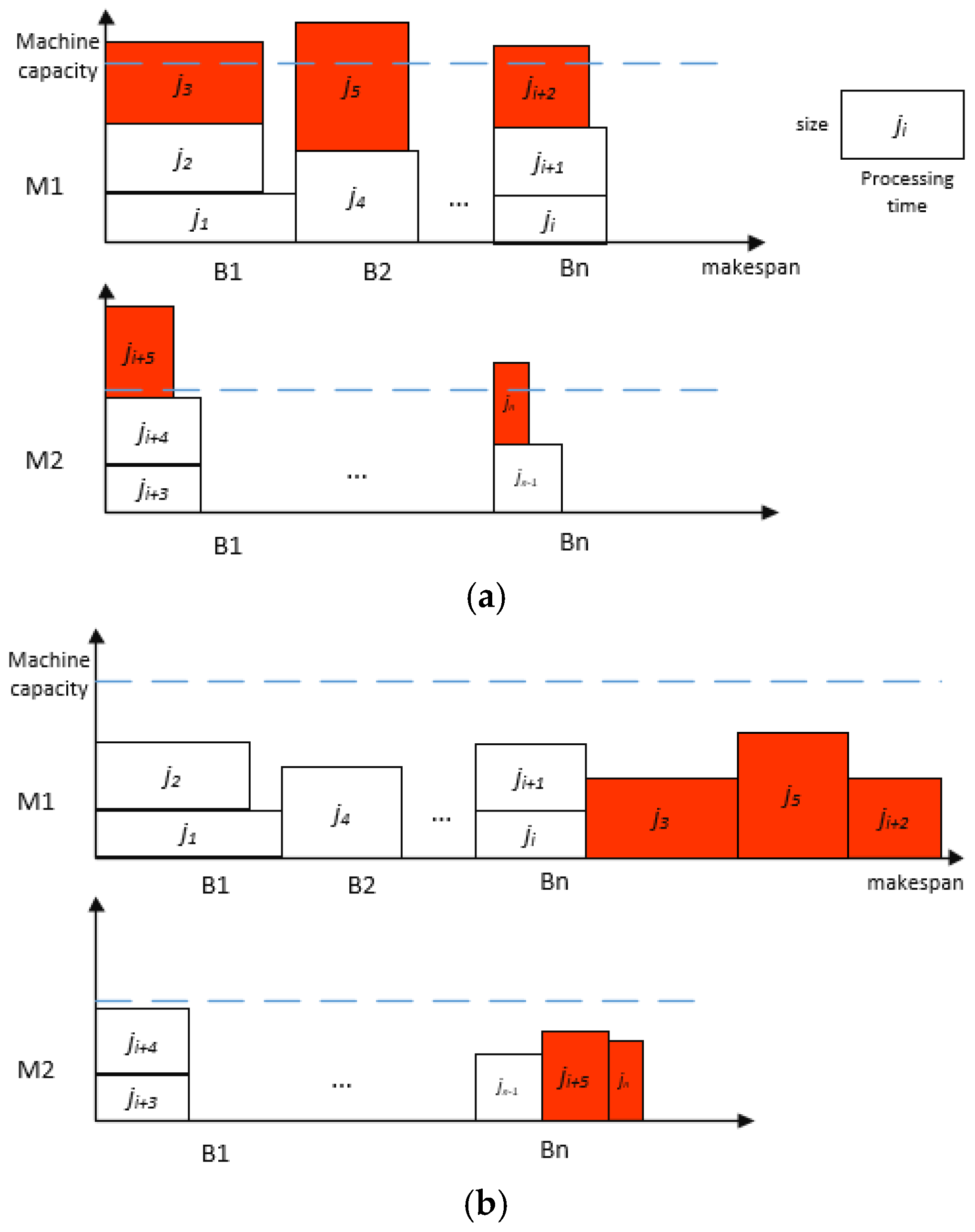
The algorithm performs a binary search within the range [ L B , U B ] . Finally, we will get a schedule with one-job-overfull batches (Figure 1a) whose makespan is at most 9 O P T / 4 . We can turn it into a viable scheduling solution (Figure 1b), where the maximum completion time is 9 O P T / 2 , as follows: for each one-job-overfull batch, move the last packed job into a new batch and calculate the new batch on the same machine. Since the iterative number could be O ( log ( j = 1 n p j ) ) , then the following theorems are obtained.
Theorem 1.
There is a 4.5-approximation algorithm for P | s j , p b a t c h , K i | C max that runs in O ( n 2 + m n log p s u m ) time, where p s u m = j = 1 n p j .
In order to achieve a strongly polynomial time algorithm, we use a technique described to modify the above algorithm slightly. Therefore, the following theorems are obtained.
Theorem 2.
There is a ( 4.5 + ε ) -approximation algorithm for P | s j , p b a t c h , K i | C max that runs in O ( n 2 + m n log ( 1 / ε ) ) time, where ε > 0 can be made arbitrarily small.

5. A 2-Approximation Algorithm for P | s j , p j = p , p b a t c h , K i | C max

In this section, we study P | s j , p j = p , p b a t c h , K i | C max , i.e., the problem of minimizing the makespan with equal processing times ( p j = p ), arbitrary job sizes (may exceed the processing power of certain batches), and non-identical machine capacities.
The 2-approximation algorithm is called LIM (largest index machine first consider). It groups the jobs in J m , J m 1 , , J 1 (this ordering is crucial), respectively, into batches greedily. During the run of the algorithm, L o a d i represents the load on machine M i , i.e., the overall processing time of the batches on M i , i = 1 , 2 , , m . The algorithm dynamically maintains a variable x , which represents the currently largest index such that L o a d x < L o a d m . If there is no such index, then we can set x = m . We can assign the next generated batch to machine M x .
Algorithm 2. LIM (largest index machine first consider)
Input: J = i = 1 m J i
Output: C max —best found solution, R T —running time
1: A s s i g n e d J S = ϕ //the jobs have been assigned to any batch
2: for i = 1   t o   m do
3: L o a d i = 0 // the load on machine M i , equals to the overall processing time of the batches on M i ,
4:end for
5:x=m
6:for i = m   t o   1 do
7: if x = = m and l o a d m > 0 then
8:   x = i
9: end if
10: create new batch b , J i = J i A s s i g n e d J S
11: for job j in J i do
12:  if b . s i z e K x then
13:   assign job j to batch b
14:    b . s i z e = b . s i z e + j . s i z e
15:   remove job from J i and add it to A s s i g n e d J S
16:  else
17:   schedule b to M x
18:    L o a d x = L o a d x + b . p
19:   initiate b
20:  end if
21: end for
22: if b is not empty and b . s i z e K x then
23:  while b . s i z e K x and J i 1 | | J i 2 | | | | J 1 A s s i g n e d J S is not empty do
24:   get first job j from J i 1 | | J i 2 | | | | J 1 A s s i g n e d J S
25:   assign job j to b
26:    b . s i z e = b . s i z e + j . s i z e
27:   remove job j from J i 1 | | J i 2 | | | | J 1 and add it to A s s i g n e d J S
28:  end while
29:  schedule b to M x
30:   L o a d x = L o a d x + b . p
31: end if
32: if L o a d x L o a d m then
33:  if x > i then
34:    x = x i
35:  else if x = = i then
36:    x = m
37:  end if
38: end if
39:end for
40:for i = 1   t o   m do
41: for batch b in M i do
42:  if b . s i z e K i then
43:   create new batch b
44:   pop the last job from b and assign it to b
45:   schedule b to M i
46:    L o a d i = L o a d i + b . p
47:  end if
48: end for
49: Update C max // append the batches scheduled on M i to C max
50:end for
51:return C max , R T = m a x ( L o a d i ) ,   i = 1 , 2 , 3 m .
Theorem 3.
Algorithm LIM is a 2-approximation algorithm for P | s j , p j = p , p b a t c h , K i | C max .
Proof. 
Let Σ 1 be the schedule with makespan S O L 1 generated by LIM after Step 2. In Σ 1 , all batches can be processed at the same time as they are assigned to a machine. During the running of the algorithm, the load on any machine is always less than or equal to the load on M m . Therefore, M m finishes last in Σ 1 . Let B l a s t be the last batch assigned to M m . Let { M l , M l + 1 , , M m } be the processing set of B l a s t , which can be defined as the largest size processing set of the job in B l a s t . In Σ 1 , let S ( B l a s t ) denote the start time of B l a s t . We have: S O L 1 = S ( B l a s t ) + p . □
Since we assigned B l a s t to M m , at that moment x = m must hold. Hence, machines M l , M l + 1 , , M m are busy in the time interval ( 0 , S ( B l a s t ) ) . All the batches allocated to machines M l , M l + 1 , , M m before S ( B l a s t ) are one-job-overfull batches. All jobs in these batches, together with the largest size job in B l a s t , must be processed on machines M l , M l + 1 , , M m in any feasible schedule. Hence, we get O P T S ( B l a s t ) + p . So we can draw the conclusion that S O L 1 O P T .
For a feasible schedule with makespan S O L generated by LIM, we have S O L 2 S O L 1 2 O P T .

6. Computational Experiments

6.1. Experimental Environment

For the performance evaluation of the 4.5-approximation and 2-approximation algorithms, all the instances are generated by a random algorithm, as in the papers [63,64,65,66,67,68]. In the process of the instances generation, five factors affecting the solution of the problem are determined: the number of jobs, the number of machines, the variation in job sizes, the variation in job processing time, and the variation in machine capacities [69,70,71,72,73,74,75].
The experiment is divided into two parts: (1) the 4.5-approximation algorithm is compared with the CPLEX result. (2) The 2-approximation algorithm is compared to CPLEX. The 4.5-approximation algorithm and 2-approximation algorithm were coded in C# and the CPLEX was programed by OPL (Optimization Programming Language), compiled, and run with the IBM ILOG CPLEX Optimization Studio 12.5.1.0 (Education Version). All the algorithms were run on the same machine (Win10, Intel (R) i7-4790, 16 GB).
First, we set the number of machines to two or four, and the capacity of each machine is represented by a uniform integer [10,40]. Then, random problem instances with number of jobs equals to 10, 20, 50, 100, 200, and 300 are generated, and each job processing time P j is generated by random sampling from a uniform distribution [1,10]. The factor settings of the experiment are summarized in Table 4.
We combine the parameters and randomly generate 50 instances for each combination (a test suite). Each test suite is denoted by a code. For instance, a test suite with 50 jobs and two machines is denoted by J3M1S1P1K1.

6.2. Comparison of 4.5-Approximation Algorithm and CPLEX

Here, a CPLEX algorithm is used to solve the MILP model given in Section 3, and we compare the CPLEX algorithm with the results of the 4.5-approximation algorithm. CPLEX always gives the optimal solution, but it cannot give the optimal solution for all instances even after operating several hours. Therefore, we set an upper execution time 1800s for CPLEX, and the best-known solution was compared. The job size and machine capacity distribution as shown in Figure 2.
Regarding the 4.5-approximation algorithm, L B and U B are initialized as follows:
L B = max ( P j ) U B = j = 1 n P j .
Figure 3 shows the result of test suite J1M1S1P1K1.
C max is the makespan of the 4.5-approximation algorithm with one-job-overfull batches and C max is the makespan of 4.5-approximation algorithm with a feasible schedule. Figure 3a shows the makespan of the 4.5-approximation algorithm with one-job-overfull batches and the algorithm with a feasible schedule. Figure 3b,c shows that the 4.5-approximation algorithm substantiates the feasibility of this research method:
C max 9 T / 4 C max 4.5 T .
Figure 3d shows that the run time of the 4.5-approximation algorithm is clearly better than CPLEX. Table 5 shows the results of all test suites. Though CPLEX is the best solver for linear programming problems, it cannot give an optimal solution for a long time, so we terminated CPLEX after running for 1800 s and used the best integer for comparison.
The results illustrate that the 4.5 approximation algorithm is more effective than CPLEX in any scale test-suite. For the small-scale test-suite (10 jobs and two machines), the best solution obtained by the 4.5-approximation algorithm is closest to the CPLEX best solution. For the medium-scale and large-scale test-suites, the average result of the 4.5-approximation algorithm is no bigger than 4.5 T .

6.3. Comparison of 2-Approximation Algorithm (LIM) and CPLEX

For the problem P | s j , p = p , p b a t c h , K i | C max , minimizing the makespan with equal running times, arbitrary job sizes (which may exceed the processing power of certain batches), and different machine capacities should be the solution. The running time of jobs was set to a default value of 8. Then, the L B and U B are denoted as
L B = 8 U B = n 8 .
Table 6 show the experimental results given by the CPLEX and the LIM algorithm for all the test suites. Column SQL-AVG (the average value of SQL) reports the average makespan obtained using the LIM algorithm. Compared with the CPLEX makespan, the LIM algorithm can obtain the efficient solution in only little running time (Column Run Times).

7. Conclusions and Future Works

The paper analyzed the parallel batch scheduling problem of minimizing the makespan, where arbitrary sizes of scheduling jobs are allowed and machines have different capacities. Each machine can only deal with jobs whose sizes do not exceed that machine’s capacity. We developed an efficient 4.5-approximation algorithm for this problem. The experimental results show that the algorithms can obtain a reasonable solution in a finite time. A 2-approximation algorithm is achieved under the particular circumstances of equivalent processing times. Computational experiments show that the fast algorithm can help to improve the efficiency of resource consumption and give researchers more choices to balance the quality of the solution and the running time in the parallel batch scheduling problem.
Several important related directions for this problem are worth researching in the future. First of all, how do we improve the fast algorithm to get closer to the optimal solution in shortest time? In addition, jobs with release times are more common BPM problems in the manufacturing industry. How to develop a fast scheduling algorithm for this problem is an import direction. Finally, BPM problems with different service levels can be considered as well.

Author Contributions

Methodology—Y.S. and B.Z., Data analysis—B.Z. and D.W., Writing—Original Draft Y.S., D.W. and K.L., Writing—Edit and Review, B.Z., Y.S., D.W., K.L. and J.X., Visualization—J.X., Funding acquisition—B.Z. All authors have read and agreed to the published version of the manuscript.

Funding

This work is supported by the CERNET Innovation Project (NGII20190605), High Education Science and Technology Planning Program of Shandong Provincial Education Department under Grant (J18KA340, J18KA385), National Natural Science Foundation of China (61976125, 61772319, 61976124, 61771087, 51605068), A Project of Shandong Province Higher Educational Science and Technology Program (No.J16LN51), the Graduate science and technology innovation fund of Shandong Technology and Business University (2018yc038), Yantai Key Research and Development Program (2019XDHZ081).

Acknowledgments

We thank the anonymous referees for their constructive comments, which helped to improve this paper.

Conflicts of Interest

The authors declare no conflict of interest.

References

  1. Marnix, K.; Van den Akker, M.; Han, H. Identifying and exploiting commonalities for the job-shop scheduling problem. Comput. Oper. Res. 2011, 38, 1556–1561. [Google Scholar]
  2. Xue, Y.; Xue, B.; Zhang, M. Self-adaptive particle swarm optimization for large-scale feature selection in classification. ACM Trans. Knowl. Discov. Data 2019, 13, 50. [Google Scholar] [CrossRef]
  3. Gahm, C.; Denz, F.; Dirr, M.; Tuma, A. Energy-efficient scheduling in manufacturing companies: A review and research framework. Eur. J. Oper. Res. 2015, 248, 744–757. [Google Scholar] [CrossRef]
  4. Deng, W.; Xu, J.; Zhao, H.M. An improved ant colony optimization algorithm based on hybrid strategies for scheduling problem. IEEE Access 2019, 7, 20281–20292. [Google Scholar] [CrossRef]
  5. Liao, C.J.; Liao, L.M. Improved MILP models for two-machine flowshop with batch processing machines. Math. Comput. Model. 2008, 48, 1254–1264. [Google Scholar] [CrossRef]
  6. Chang, P.Y. Heuristics to minimize makespan of parallel batch processing machines. Int. J. Adv. Manuf. Technol. 2008, 37, 1005–1013. [Google Scholar]
  7. Drozdowski, M. Classic scheduling theory. In Scheduling for Parallel Processing; Springer: London, UK, 2009; pp. 55–86. [Google Scholar]
  8. Deng, W.; Zhao, H.; Yang, X.; Xiong, J.; Sun, M.; Li, B. Study on an improved adaptive PSO algorithm for solving multi-objective gate assignment. Appl. Soft Comput. 2017, 59, 288–302. [Google Scholar] [CrossRef]
  9. Guo, S.K.; Liu, Y.Q.; Chen, R.; Sun, X.; Wang, X. Improved SMOTE algorithm to deal with imbalanced activity classes in smart homes. Neural Process. Lett. 2019, 50, 1503–1526. [Google Scholar] [CrossRef]
  10. Li, X.; Xie, Z.; Wu, J.; Li, T. Image encryption based on dynamic filtering and bit cuboid operations. Complexity 2019, 2019, 7485621. [Google Scholar] [CrossRef]
  11. Deng, W.; Zhao, H.M.; Zou, L.; Li, G.; Yang, X.; Wu, D. A novel collaborative optimization algorithm in solving complex optimization problems. Soft Comput. 2017, 21, 4387–4398. [Google Scholar] [CrossRef]
  12. Kim, S.; Kim, J.K. A method to construct task scheduling algorithms for heterogeneous multi-core systems. IEEE Access 2019, 7. [Google Scholar] [CrossRef]
  13. Leung, Y.T.; Li, C.L. Scheduling with processing set restrictions: A survey. Int. J. Prod. Econ. 2008, 116, 251–262. [Google Scholar] [CrossRef] [Green Version]
  14. Su, J.; Sheng, Z.; Leung, V.C.M.; Chen, Y. Energy efficient tag identification algorithms for RFID: Survey, motivation and new design. IEEE Wirel. Commun. 2019, 67, 118–124. [Google Scholar] [CrossRef]
  15. Luo, J.; Chen, H.; Heidari, A.A.; Xu, Y.; Zhang, Q.; Li, C. Multi-strategy boosted mutative whale-inspired optimization approaches. Appl. Math. Model. 2019, 73, 109–123. [Google Scholar] [CrossRef]
  16. Fu, H.; Wang, M.; Li, P.; Jiang, S.; Hu, W.; Guo, X.; Cao, M. Tracing knowledge development trajectories of the internet of things domain: A main path analysis. IEEE Trans. Ind. Inform. 2019, 15. [Google Scholar] [CrossRef]
  17. Su, J.; Sheng, Z.; Liu, A.X.; Han, Y.; Chen, Y. A group-based binary splitting algorithm for UHF RFID anti-collision systems. IEEE Trans. Commun. 2019. [Google Scholar] [CrossRef] [Green Version]
  18. Liu, Y.; Yi, X.; Chen, R.; Hai, Z.; Gu, J. Feature extraction based on information gain and sequential pattern for English question classification. IET Softw. 2018, 12, 520–526. [Google Scholar] [CrossRef]
  19. Yu, H.; Zhao, N.; Wang, P.; Chen, H.; Li, C. Chaos-enhanced synchronized bat optimizer. Appl. Math. Model. 2020, 77, 1201–1215. [Google Scholar] [CrossRef]
  20. Li, H.; Gao, G.; Chen, R.; Ge, X.; Guo, S.; Hao, L.Y. The influence ranking for testers in bug tracking systems. International. Int. J. Softw. Eng. Knowl. Eng. 2019, 29, 93–113. [Google Scholar] [CrossRef]
  21. Uzsoy, R. Scheduling a single batch processing machine with non-identical job sizes. Int. J. Prod. Res. 1994, 32, 1615–1635. [Google Scholar] [CrossRef]
  22. Zhang, G.; Cai, X.; Lee, C.Y.; Wong, C. Minimizing makespan on a single batch processing machine with nonidentical job sizes. Naval Res. Logist. 2001, 48, 226–240. [Google Scholar] [CrossRef]
  23. Dosa, G.; Tan, Z.; Tuza, Z.; Yan, Y.; Lányi, C.S. Improved bounds for batch scheduling with nonidentical job sizes. Naval Res. Logist. 2014, 61, 351–358. [Google Scholar] [CrossRef]
  24. Li, S.; Li, G.; Wang, X.; Liu, Q. Minimizing makespan on a single batching machine with release times and non-identical job sizes. Oper. Res. Lett. 2005, 33, 157–164. [Google Scholar] [CrossRef]
  25. Chang, P.Y.; Damodaran, P.; Melouk, S. Minimizing makespan on parallel batch processing machines. Int. J. Prod. Res. 2004, 42, 4211–4220. [Google Scholar] [CrossRef]
  26. Cheng, B.; Yang, S.; Hu, X.; Chen, B. Minimizing makespan and total completion time for parallel batch processing machines with non-identical job sizes. Appl. Math. Model. 2012, 36, 3161–3167. [Google Scholar] [CrossRef]
  27. Chung, S.; Tai, Y.; Pearn, W. Minimisingmakespan on parallel batch processing machines with non-identical ready time and arbitrary job sizes. Int. J. Prod. Res. 2009, 47, 5109–5128. [Google Scholar] [CrossRef]
  28. Ozturk, O.; Espinouse, M.L.; Mascolo, M.D.; Gouin, A. Makespanminimisation on parallel batch processing machines with non-identical job sizes and release dates. Int. J. Prod. Res. 2012, 50, 1–14. [Google Scholar] [CrossRef]
  29. Li, S. Makespan minimization on parallel batch processing machines with release times and job sizes. J. Softw. 2012, 7, 1203–1210. [Google Scholar] [CrossRef]
  30. Costa, A.; Cappadonna, F.A.; Fichera, S. A novel genetic algorithm for the hybrid flow shop scheduling with parallel batching and eligibility constraints. Int. J. Adv. Manuf. Technol. 2014, 75, 833–847. [Google Scholar] [CrossRef]
  31. Wang, H.M.; Chou, F.D. Solving the parallel batch-processing machines with different release times, job sizes, and capacity limits by metaheuristics. Expert Syst. Appl. 2010, 37, 1510–1521. [Google Scholar] [CrossRef]
  32. Damodaran, P.; Diyadawagamage, D.A.; Ghrayeb, O.; Vélez-Gallego, M.C. A particle swarm optimization algorithm for minimizing makespan of nonidentical parallel batch processing machines. Int. J. Adv. Manuf. Technol. 2012, 58, 1131–1140. [Google Scholar] [CrossRef]
  33. Jia, Z.H.; Li, K.; Leung, J.Y.T. Effective heuristic for makespan minimization in parallel batch machines with non-identical capacities. Int. J. Prod. Econ. 2015, 169, 1–10. [Google Scholar] [CrossRef]
  34. Wang, J.Q.; Leung, J.Y.T. Scheduling jobs with equal-processing-time on parallel machines with non-identical capacities to minimize makespan. Int. J. Prod. Econ. 2014, 156, 325–331. [Google Scholar] [CrossRef]
  35. Li, S. Approximation algorithms for scheduling jobs with release times and arbitrary sizes on batch machines with non-identical capacities. Eur. J. Oper. Res. 2017, 263, 815–826. [Google Scholar] [CrossRef]
  36. He, Z.; Shao, H.D.; Zhang, X.Y.; Cheng, J.S.; Yang, Y. Improved deep transfer auto-encoder for fault diagnosis of gearbox under variable working conditions with small training samples. IEEE Access 2019, 7, 115368–115377. [Google Scholar] [CrossRef]
  37. Zhao, H.M.; Liu, H.D.; Xu, J.J.; Deng, W. Performance prediction using high-order differential mathematical morphology gradient spectrum entropy and extreme learning machine. IEEE Trans. Instrum. Meas. 2019. [Google Scholar] [CrossRef]
  38. Deng, X.; Feng, H.; Li, G.; Shi, B. A PTAS for semiconductor burn-in scheduling. J. Comb. Optim. 2005, 9, 5–17. [Google Scholar] [CrossRef]
  39. Liu, R.; Wang, H.; Yu, X.M. Shared-nearest-neighbor-based clustering by fast search and find of density peaks. Inf. Sci. 2018, 450, 200–226. [Google Scholar] [CrossRef]
  40. Hu, B.; Wang, H.; Yu, X.; Yuan, W.; He, T. Sparse network embedding for community detection and sign prediction in signed social networks. J. Ambient Intell. Humaniz. Comput. 2019, 10, 175–186. [Google Scholar] [CrossRef]
  41. Zhao, H.M.; Zheng, J.J.; Xu, J.J.; Deng, W. Fault diagnosis method based on principal component analysis and broad learning system. IEEE Access 2019, 7, 99263–99272. [Google Scholar] [CrossRef]
  42. Xu, Y.; Chen, H.; Heidari, A.A.; Luo, J.; Zhang, Q.; Zhao, X.; Li, C. An efficient chaotic mutative moth-flame-inspired optimizer for global optimization tasks. Expert Syst. Appl. 2019, 129, 135–155. [Google Scholar] [CrossRef]
  43. Su, J.; Sheng, Z.; Xie, L.; Li, G.; Liu, A.X. Fast splitting based tag identification algorithm for anti-collision in UHF RFID system. IEEE Trans. Commun. 2019, 67, 2527–2538. [Google Scholar] [CrossRef] [Green Version]
  44. Liu, W.; Li, H.; Zhu, H.; Xu, P. Properties of a steel slag-permeable asphalt mixture and the reaction of the steel slag-asphalt interface. Materials 2019, 12, 3603. [Google Scholar] [CrossRef] [PubMed] [Green Version]
  45. Zhou, J.; Du, Z.; Yang, Z.; Xu, Z. Dynamic parameters optimization of straddle-type monorail vehicles based multiobjective collaborative optimization algorithm. Veh. Syst. Dyn. 2019, 41, 1–21. [Google Scholar] [CrossRef]
  46. Li, T.; Shi, J.; Li, X.; Wu, J.; Pan, F. Image encryption based on pixel-level diffusion with dynamic filtering and dna-level permutation with 3D Latin cubes. Entropy 2019, 21, 319. [Google Scholar] [CrossRef] [Green Version]
  47. Wang, Z.; Pu, J.; Cao, L.; Tan, J. A parallel biological optimization algorithm to solve the unbalanced assignment problem based on DNA molecular computing. Int. J. Mol. Sci. 2015, 16, 25338–25352. [Google Scholar] [CrossRef] [Green Version]
  48. Kang, L.; Zhao, L.; Yao, S.; Duan, C. A new architecture of super-hydrophilic beta-SiAlON/graphene oxide ceramic membrane for enhanced anti-fouling and separation of water/oil emulsion. Ceram. Int. 2019, 45, 16717–16721. [Google Scholar] [CrossRef]
  49. Liu, Y.; Mu, Y.; Chen, K.; Li, Y.; Guo, J. Daily activity feature selection in smart homes based on pearson correlation coefficient. Neural Process. Lett. 2020. [Google Scholar] [CrossRef]
  50. Liu, G.; Liu, D.; Liu, J.; Gao, Y.; Wang, Y. Asymmetric temperature distribution during steady stage of flash sintering dense zirconia. J. Eur. Ceram. Soc. 2018, 38, 2893–2896. [Google Scholar] [CrossRef]
  51. Ren, Z.; Skjetne, R.; Jiang, Z.; Gao, Z.; Verma, A.S. Integrated GNSS/IMU hub motion estimator for offshore wind turbine blade installation. Mech. Syst. Signal Process. 2019, 123, 222–243. [Google Scholar] [CrossRef]
  52. Chen, H.; Jiao, S.; Heidari, A.A.; Wang, M.; Chen, X.; Zhao, X. An opposition-based sine cosine approach with local search for parameter estimation of photovoltaic models. Energy Convers. Manag. 2019, 195, 927–942. [Google Scholar] [CrossRef]
  53. Liu, D.; Cao, Y.; Liu, J.; Gao, Y.; Wang, Y. Effect of oxygen partial pressure on temperature for onset of flash sintering 3YSZ. J. Eur. Ceram. Soc. 2018, 38, 817–820. [Google Scholar] [CrossRef]
  54. Wang, H.; Song, Y.Q.; Wang, L.T.; Hu, X.H. Memory model for web ad effect based on multi-modal features. J. Assoc. Inf. Sci. Technol. 2019, 4, 1–14. [Google Scholar]
  55. Xu, Y.; Chen, H.; Luo, J.; Zhang, Q.; Jiao, S.; Zhang, X. Enhanced Moth-flame optimizer with mutation strategy for global optimization. Inf. Sci. 2019, 492, 181–203. [Google Scholar] [CrossRef]
  56. Chen, R.; Guo, S.K.; Wang, X.Z.; Zhang, T.L. Fusion of multi-RSMOTE with fuzzy integral to classify bug reports with an imbalanced distribution. IEEE Trans. Fuzzy Syst. 2019, 27. [Google Scholar] [CrossRef]
  57. Heidari, A.; Mirjalili, S.; Faris, H.; Aljarah, I.; Mafarja, M.; Chen, H. Harris hawks optimization: Algorithm and applications. Future Gener. Comput. Syst. 2019, 97, 849–872. [Google Scholar] [CrossRef]
  58. Ou, J.; Leung, J.Y.T.; Li, C.L. Scheduling parallel machines with inclusive processing set restrictions. Naval Res. Logist. 2008, 55, 328–338. [Google Scholar] [CrossRef]
  59. Li, S. Parallel batch scheduling with inclusive processing set restrictions and non-identical capacities to minimize makespan. Eur. J. Oper. Res. 2017, 260, 12–20. [Google Scholar] [CrossRef]
  60. Fu, H.; Manogaran, G.; Wu, K.; Cao, M.; Jiang, S.; Yang, A. Intelligent decision-making of online shopping behavior based on internet of things. Int. J. Inf. Manag. 2019, 50. [Google Scholar] [CrossRef]
  61. Li, T.; Hu, Z.; Jia, Y.; Wu, J.; Zhou, Y. Forecasting crude oil prices using ensemble empirical mode decomposition and sparse Bayesian learning. Energies 2018, 11, 1882. [Google Scholar] [CrossRef] [Green Version]
  62. Wang, Z.; Ren, X.; Ji, Z.; Huang, W.; Wu, T. A novel bio-heuristic computing algorithm to solve the capacitated vehicle routing problem based on Adleman–Lipton model. Biosystems 2019, 184, 103997. [Google Scholar] [CrossRef]
  63. Ham, A.; Fowler, J.W.; Cakici, E. Constraint programming approach for scheduling jobs with release times, non-identical sizes, and incompatible families on parallel batching machines. IEEE Trans. Semicond. Manuf. 2017, 30, 500–507. [Google Scholar] [CrossRef]
  64. Sun, F.R.; Yao, Y.D.; Li, G.Z.; Liu, W. Simulation of real gas mixture transport through aqueous nanopores during the depressurization process considering stress sensitivity. J. Pet. Sci. Eng. 2019, 178, 829–837. [Google Scholar] [CrossRef]
  65. Deng, W.; Xu, J.; Song, Y.; Zhao, H. An effective improved co-evolution ant colony optimization algorithm with multi-strategies and its application. Int. J. Bio-Inspired Comput. 2019. [Google Scholar]
  66. Wang, Z.; Ji, Z.; Wang, X.; Wu, T.; Huang, W. A new parallel DNA algorithm to solve the task scheduling problem based on inspired computational model. BioSystems 2017, 162, 59–65. [Google Scholar] [CrossRef] [PubMed]
  67. Wu, J.; Shi, J.; Li, T. A novel image encryption approach based on a hyperchaotic system, pixel-level filtering with variable kernels, and DNA-level diffusion. Entropy 2020, 22, 5. [Google Scholar] [CrossRef] [Green Version]
  68. Peng, Y.; Lu, B.L. Discriminative extreme learning machine with supervised sparsity preserving for image classification. Neurocomputing 2017, 261, 242–252. [Google Scholar] [CrossRef]
  69. Xu, J.; Chen, R.; Deng, W.; Zhao, H. An infection graph model for reasoning of multiple faults in software. IEEE Access 2019, 7, 77116–77133. [Google Scholar] [CrossRef]
  70. Zhou, J.; Du, Z.; Yang, Z.; Xu, Z. Dynamics study of straddle-type monorail vehicle with single-axle bogies based full-scale rigid-flexible coupling dynamic model. IEEE Access 2019, 7, 2169–3536. [Google Scholar] [CrossRef]
  71. Shao, H.; Cheng, J.; Jiang, H.; Yang, Y.; Wu, Z. Enhanced deep gated recurrent unit and complex wavelet packet energy moment entropy for early fault prognosis of bearing. Knowl. Based Syst. 2019. [Google Scholar] [CrossRef]
  72. Li, T.; Yang, M.; Wu, J.; Jing, X. A novel image encryption algorithm based on a fractional-order hyperchaotic system and DNA computing. Complexity 2017, 2017, 9010251. [Google Scholar] [CrossRef] [Green Version]
  73. Zhao, H.; Zheng, J.; Deng, W.; Song, Y. Semi-supervised broad learning system based on manifold regularization and broad network. IEEE Trans. Circuits Syst. I Regul. Pap. 2019. [Google Scholar] [CrossRef]
  74. Li, T.; Zhou, Y.; Li, X.; Wu, J.; He, T. Forecasting daily crude oil prices using improved CEEMDAN and ridge regression-based predictors. Energies 2019, 12, 3603. [Google Scholar] [CrossRef] [Green Version]
  75. Liu, Y.Q.; Wang, X.X.; Zhai, Z.G.; Chen, R.; Zhang, B.; Jiang, Y. Timely daily activity recognition from headmost sensor events. ISA Trans. 2019, 94, 379–390. [Google Scholar] [CrossRef] [PubMed]
Figure 1. Illustration of the 4.5-approximation algorithm. (a) The 4.5-approximation algorithm with one-job-overfull batches. (b) The 4.5-approximation algorithm with a feasible schedule.
Applsci 10 00460 g001
Figure 2. Job size and machine capacity distribution.
Applsci 10 00460 g002
Figure 3. Results of J1M1S1P1K1. (a) Comparison makespan of CPLEX and the 4.5-approximation algorithm with one-job-overfull batches and the 4.5-approximation algorithm with a feasible schedule. (b) Comparison makespan of the 4.5-approximation algorithm with one-job-overfull batches and 9 T / 4 . (c) Comparison makespan of the 4.5-approximation algorithm with a feasible schedule and 4.5T. (d) Comparison running time of CPLEX and the 4.5-approximation algorithm with one-job-overfull batches and the 4.5-approximation algorithm with a feasible schedule.
Applsci 10 00460 g003aApplsci 10 00460 g003b
Table 1. Notations.
Table 1. Notations.
NotationDescription
J set of jobs, J = { J 1 , J 2 , , J n }
J j jth job
p j processing time of job J j
s j size of job J j
set of machines, = { M 1 , M 2 , , M m }
M i ith machine
K i capacities of M i
B i , g g th batch scheduled on ith machine
U B upper bound of makespan
L B lower bound of makespan
C max makespan
Table 2. Indices.
Table 2. Indices.
IndicesDescription
i index of machine, i = { 1 , 2 , , m }
j index of job, j = { 1 , 2 , , n }
l index of batch, l = { 1 , 2 , , n }
Table 3. Decision variables.
Decision VariablesDescription
x j i l 1, if job J j is assigned to the l th batch processed on machine M i ; 0, otherwise.
y i l the processing time of l th batch processed on machine M i .
C max makespan.
Table 4. Factors setting of the experiment.
FactorsLevels
Number of jobs (n)10, 20, 50, 100, 200, 300
Number of machines (m)2, 4
Size of jobs (s)[1,10], [ 11 , max ( K i ) ]
Processing time of jobs (P)[1,10]
Capacity of machines (K)[10,40]
Table 5. Simulation results of CPLEX and the 4.5-approximation algorithm with one-job-overfull batches and a feasible schedule.
Test SuiteCPLEX C max C max T 9 T / 4 4.5 T
MakespanGAP (%)Run Time (s)BestAVGWorstRun Time (s)BestAVGWorstRun Time (s)
J1M1S1P1K1900.02914.92210.021023.23340.029.4921.3542.71
J1M2S1P1K1800.09913.02220.02919.06360.029.6321.6643.32
J2M1S1P1K11942.112.101721.62270.013035.76510.0110.2623.1046.19
J2M2S1P1K11040.002.261519.44220.012432.04480.0110.0922.745.4
J3M1S1P1K15279.87466.473547.39680.136186.611360.1321.8649.1998.37
J3M2S1P1K14780.8525.392128.84400.023753.531060.0213.5730.5361.07
J4M1S1P1K15990.6818007694.571290.04150175.82550.0442.7396.14192.29
J4M2S1P1K12986.2118004052.751080.047699.201800.0424.2254.50108.99
J5M1S1P1K119797.461800151185.532550.08250352.334960.0883.29187.40374.81
J5M2S1P1K1--180078105.491860.08146203.963650.0847.55106.99213.98
J6M1S1P1K116197.21800213283.433870.12377535.717390.12126.65284.96569.93
J6M2S1P1K1--1800104143.732830.12190275.355600.1364.65145.46290.93
1 Note: (1) Column 2 is the minimum makespan of 50 instances for each test suite. ‘-’ represents that CPLEX could not find a feasible solution in 1800 s. (2) Each test suite contains 50 instances. Columns 5, 6, and 7 report the best, average, and worst C max , respectively. Columns 9, 10, and 11 report the best, average, and worst C max , respectively. (3) Columns 13, 14, and 15 report the average T , 9 T / 4 , and 4.5 T of 50 instances, respectively.
Table 6. Simulation results of CPLEX and the 2-approximation algorithm with one-job-overfull batches and a feasible schedule.
Test SuiteCPLEXSOL 1SOL
MakespanGAP (%)Run Time (s)BestAVGWorstRun Time (s)BestAVGWorstRun Time (s)
J1M1S1P1K12400.251618.822402431.84480
J1M2S1P1K12466.670.2089.101601617.10340
J2M1S1P1K14013.933.112438.275604466.20880
J2M2S1P1K12433.332.131623.224003242.04720
J3M1S1P1K18087.0618006489.411200112159.532240
J3M2S1P1K16487.538.344061.9696072109.961600
J4M1S1P1K120096306.73136186.672320240337.734320
J4M2S1P1K114495.83180080121.251920136219.613440
J5M1S1P1K141298.591800264374.124560480679.068480
J5M2S1P1K1--1800160245.493360296453.026560
J6M1S1P1K1--1800424569.1074407441031.3713600
J6M2S1P1K1--1800232343.225120416633.579440
1 Note: When run time is labeled as 0, it was less than 10−2.

