Identification of Players Ranking in E-Sport

Abstract

Human activity is moving steadily to virtual reality. More and more, people from all over the world are keen on growing fascination with e-sport. In practice, e-sport is a type of sport in which players compete using computer games. The competitions in games, like FIFA, Dota2, the League of Legends, and Counter-Strike, are prestigious tournaments with a global reach and a budget of millions of dollars. On the other hand, reliable player ranking is a critical issue in both classic and e-sport. For example, the “Golden Ball” is the most valuable prize for an individual football player in the whole football history. Moreover, the entire players’ world wants to know who the best player is. The position of each player in the ranking depends on the assessment of his skills and predispositions. In this paper, we studied identification of players evaluation and ranking obtained using the multiple-criteria decision-making based method called Characteristic Objects METhod (COMET) on the example of the popular game Counter-Strike: Global Offensive (CS: GO). We present a range of advantages of the player evaluation model created using the COMET method and, therefore, prove the practicality of using multi-criteria decision analysis (MCDA) methods to build multi-criteria assessment models in emerging areas of eSports. Thus, we provide a methodical and practical background for building a decision support system engine for the evaluation of players in several eSports.

1. Introduction

Sport has always played an essential role in every culture in the past and still does in current times. Everybody knows conventional sports, such as football, volleyball, basketball, etc., but there are new sports appearing that are increasingly expanding in popularity. One of them is Electronic Sports, also known as eSports or e-sports [1]. At the beginning of the 90s, the history of e-sport began. During this decade, it became more and more popular, and the number of players increased significantly [2,3,4,5]. E-sport is a type of sport in which players compete in computer games [6,7]. The players’ activities are only restrained from being placed in the virtual environment [3]. E-sport is exciting entertainment for many fans, but it is also a source of income for the professional players and the whole e-sport organization. Professional players usually belong to different e-sport organizations and represent their teams competing in omnifarious tournaments, events, and international championship [2,3,4,8]. The competition takes place online or through so-called local networks (LAN). The most encounters take place in a LAN network, where both smaller and larger numbers of computers are connected in one building allowed for lower in-game latency between gamers [2,6,8,9,10]. In e-sports, the viewership is crucial. The gameplay should be designed to attract and emotionally engage the participation of as many gameplay observers as possible.

E-sport is a lifestyle for computer gamers. It becomes a real career path from which you can start, develop, and build your future. People still consider e-sport very conservatively. They think of it as something trivial and frivolous. While some people do not take it seriously all the time, spectator count records, as well as prize pool records, are regularly updated during major tournaments, reaching millions watching Counter-Strike: Global Offensive (CS: GO) [11]. It is full of opportunities, awards, travel, and also requires great sacrifice. It is incredibly demanding to reach a world-class level [1]. Actually, it looks like a full-time job. Players usually train 8 hours a day or more. They use the computer as a tool to achieve success in a new field. To become a professional, people have to work hard without any excuses. A player is considered as professional when he is hired by an organization that pays for his work representing that entity by appearing at events, mostly official tournaments on a national or international level [8]. E-sport has become an area that requires so much precision that even milliseconds determine whether to win or lose. Pointing out the importance of specialized skills, such as hand-eye coordination, muscle memory, or reaction time, as well as strategical or tactical in-game knowledge, increases achieving success in that area [12]. Hand-eye coordination is the ability of the vision system to coordinate the information received through the eyes to control, guide, and direct the hands in the accomplishment of a given task, such as handwriting or catching a ball [13]. The aim of e-sports is defeating other players. It could be done by neutralizing them, or just like in sports games, by racing as fast as possible to cross the finish line before your opponents. In addition, the win may be achieved by scoring the most points [2,3].

One of the most popular genres of eSports games is First-Person-Shooter (FPS) [2,6,8,14]. The virtual environment of the game is approached from the perspective of the avatar. The only thing visible of the avatars on the screen is the hands and the weapons they handle [2]. Counter-Strike is an FPS multiplayer game created and released by Valve Corporation and Hidden Path Entertainment [5,6]. There were many other versions of the game, which did not achieve much success. Valve realized how popular e-sport had become and create the new Counter-Strike game we play today, wholly tailored for competition, known as CS: GO. The rules in CS: GO are uncomplicated. There are two teams in the game: terrorists (T) and counter-terrorists (CT). Each team aims to eliminate the opposing team or to perform a specific task. The first one’s target is to plant the bomb and let it explode, while the second’s is to prevent the bomb from being planted and/or exploding. Additionally, the game consists of 30 rounds, where each last about 2 min. After 15 rounds, players need to switch teams. Then, the team that first achieves 16 rounds is the winner. When the game does not end in 30 rounds, it goes to overtime. It consists of a best of six rounds, three on each side. The team that gets to 4 rounds wins. If there is another draw situation, the same rule applies until a winner is found [4,8]. The team’s economy is concerned with the amount of money that everybody on the team have pooled cooperatively in order to buy new weapons and equipment. Winning a round by eliminating the entire enemy team provides the winners with USD 3250 per player, plus USD 300 if the bomb is planted by a terrorist. Winning by time on the counter-terrorist’s side rewards players USD 3250, and winning the round with a defusal (CT) or detonation of the bomb (T) rewards USD 3500. However, if the terrorists run out of time before killing all the oponnents or planting the bomb, they will not come in for any cash prize. If a round is lost on the T-side, but they still manage to plant the bomb, the team will be awarded USD 800 in addition to the current round loss streak value. The money limit for each individual player in competitive matches is equal to USD 16.000 [15].

For gamers, the foundation of e-sports is the glory of winning, the ability to evoke excitement in people, and the privilege of being perceived as one of the best players in the world [2,8]. In the past, players had to bring their equipment to LAN events, while having fun in a hermetically sealed society. They could then eventually win small cash prizes or gadgets. Now, these players are winning a prize pool of over USD 500 thousand, performing on big stages full of cameras and audience [1]. The increase in popularity of e-sports was not only impressive but also forced many business people, large corporations, and television companies to become interested in this dynamically developing market [8]. E-sport teams are often headed by traditional sports organizations and operated by traditional sports media. Tournaments are organized by conventional sports leagues highlighting the growing connections between classical sport and e-sport [16].

In recent years, e-sport has become one of the fastest-growing forms of new media driven by the growing origins of games broadcasting technologies [7,17]. E-sport and computer gaming have entered the mainstream, transforming into a convenient way of entertainment. In 2019, 453.8 million people had been watching e-sport worldwide, which increased by about 15% compared to 2018. It consisted of 201 million regular and 252 million occasional viewers. Between 2019 and 2023, total e-sport viewership is expected to increase by 9% per year, from 454 million in 2019 to 646 million in 2023. In six years, the number of watchers will almost double, reaching 335 million in 2017. In the current economic situation, global revenues from e-sport may reach USD 1.8 billion by 2022, or even an optimistic USD 3.2 billion. Hamari in Reference [3] claims that with the development of e-sport, classic sport is becoming a computer-based form of media and information technology. Therefore, e-sport is a fascinating subject of research in the field of information technology.

The accurate player ranking is a crucial issue in both classic [18] and e-sport [19,20]. The result of a classification, calculated based on wins and losses in a competitive game, is often considered to be an indicator of a player’s skills [20]. Each player’s position in the ranking is strictly determined by their abilities, predispositions, and talent in the field of represented discipline [16]. However, there are more than just statistics to prove the player’s value and ability. Many professional players play a supporting role in their teams, and winning even a single round is a priority. What matters first and foremost is the team’s victory, unlike the ambitions of the individual units. The team members have to work collectively, like one organism, and everyone has to cooperate to achieve the team’s success and the best possible results [21]. That is why the creation of accurate player ranking is a problematic issue.

In this paper, we identify the model to generate a ranking of players in the popular e-sport game, i.e., Counter-Strike: Global Offensive (CS: GO), using the Characteristic Objects METhod (COMET). The obtained ranking will be compared to Rating 2.0, which is the most popular for CS: GO game [22,23]. This study case facilitates the application of COMET in the new field of application. The COMET is a novel method of identifying a multi-criteria expert decision model to solve decision problems based on a rule set, using elements of the theory of fuzzy sets [23,24]. Unlike most available multi-criteria decision analysis (MCDA) methods, COMET is completely free of the rank reversal problem. The advantages of this technique are both an intuitive dialogue with the decision-maker and the identification of a complete model of the modeling area, which is a vital element in the application of the proposed approach in the methodological and algorithmic engine in the area of computer games and, more specifically, e-sport.

The most important methodological contribution is the analysis of the significance of individual inputs and outputs, which enables the analysis of the dependence of results on individual input data. Similarly, as in the Analytic Hierarchy Process (AHP) method, it is to serve as a possibility of extended decision analyzing in order to explain what influence particular aspects had on the final result. The Spearman correlation coefficient is used to measure the input-output dependencies, which extends the COMET technique to include new interpretative possibilities. It is important to note that this is significant as the COMET method itself does not apply any significance weights. The proposed approach makes it possible to estimate the significant weights.

The justification of the undertaken research has both theoretical and practical dimensions. MCDA methods themselves have proved to be powerful tools to solve different practical problems [25,26]. In particular, the construction of assessment models and rankings using MCDA methods is extensively discussed in the literature [27,28,29,30]. Examples of decision-making problems successfully solved with the usage of different multi-criteria methods include the assessment of environmental effects of marine transportation [31], innovation [32,33], sustainability [34,35], evaluation of renewable energy sources (RES) investments [36,37] or a broad environmental investments assessment [38], and industrial [39], as well as personnel assessment [40] of preventive health effects [41] or even evaluation of medical therapy effects [42,43]. It is also worth noticing the additional motivation of the research that MCDA methods have already shown their utility in building assessment models in traditional sports. For instance, the MCDA-based evaluation of soccer players was conducted in Reference [44], where Choquet method was used to evaluate the performance of sailboats [45]. Preference ranking organization method for enrichment evaluation II (PROMETHEE II)-based evaluation model of football clubs was proposed in Reference [46], while application of AHP/SWOT model in sport marketing was presented in Reference [47]. MCDA-based, multi-stakeholder perspective was handled in the evaluation of national-level sport organizations in Reference [48]. Both the examples provided and state of the art presented in Reference [49] clearly show the critical role of MCDA methods in the area of building assessment models and rankings in the field of sport. When we analyze the area of the e-sport in addition to the dominant trends, including economic research [50], sociological [3,51], psychological [52] or conversion-oriented research, and user experience (UX) [53], we observe attempts to use quantitative methods in the search for the algorithmic engines of digital products and games. For example, ex-post surveys and statistical-based approach were used to manage the health of the eSport athlete [54]. Personal branding of eSports athletes was evaluated in Reference [55]. In Reference [56], streaming-based performance indicators were developed, and players’ behavior and performance were assessed. The research focused on win/live prediction in multi-player games was conducted in Reference [57]. The study aimed to identify the biometric features contributing to the classification of particular skills of the players was presented in Reference [58]. So, far, only one example of MCDA-based method usage in e-sport player selection and evaluation has been proposed [58]. The authors indicate the appropriateness of fuzzy MCDA in the domain of e-sport player selection and assessment. The above literature studies show a distinct research gap, including the limited application of MCDA in e-sport domain. Besides, the paper addresses the following essential theoretical and practical research gaps:

• extension of the COMET method by the stage of analyzing the significance of individual input data and decision-making sub-models to the final form of a ranking of decision-making options
• transferring the methodological experience of using MCDA methods to the important and promising ground for building decision support systems in the area of eSports;
• by identifying a domain-specific proper reflecting modeling domain (e-sport player evaluation), the form of which (both within the family of evaluation criteria and alternatives) is significantly different from that of classical sports; and
• analysis and study of the adaptation and examination of MCDA methods usage as an algorithmic methodological engine of decision support system (potentially providing additional functionality to a range of available digital products and games).

The rest of the paper is organized as follows: MCDA foundations and simple comparison of MCDA techniques are presented in Section 2. Section 3 contains preliminaries of the fuzzy sets theory. The explanation of the definitions and algorithms of the multi-criteria decision-making method named COMET is given in Section 4. Section 5 introduces the results of the study, and, in Section 6, the discussion about the differences in both rankings. In Section 7, we present the conclusions and future directions.

2. MCDA Fundations

Multi-criteria decision support aims to achieve a solution for the most satisfactory decision-maker and at the same time to meet a sufficient number of often conflicting goals [59]. The search for such solutions requires the consideration of many alternatives and their evaluation against many criteria, as well as the transfer of the subjectivity of evaluation (e.g., the relevance of the criteria by the decision-maker) into a target model. Multi-criteria Decision Analysis (MCDA) methods is dedicated to solving this class of decision problems. During many years of research, two schools of MCDA methods have been developed. First, American MCDA school is based on the assumption that the decision-maker’s preferences are expressed using two basic binary relations. When comparing the decision-making options, undifferentiated relations and preferences may occur. In the case of the European MCDA school, this set has been significantly extended by introducing the so-called “superiority relationship”. The relation of superiority, apart from the two basic relations mentioned above, introduces the relation of weak preference of one of the variants to another and the relation of incomparability of the decision options.

In the case of the American school methods, the result of the comparison of variants is determined for each criterion separately, and the effect of the aggregation of the grades is a single, synthesized criterion, with the order of variants being full. The methods of the American school of decision support in the vast majority using the function of value or utility. The best-known methods of the American school are Multi Attribute Utility Theory (MAUT), AHP, Analytic Network Process (ANP), Simple Multi-Attribute Rating Technique (SMART), UTA, Simple Multi-Attribute Rating Technique (MACBETH), or Technique for Order of Preference by Similarity to Ideal Solution (TOPSIS).

In contrast to the American school (which is at the same time an accusation of “European School”-oriented researchers), the algorithms of the European School methods are strongly oriented on faithful reflection of the decision-maker’s preferences (including their imprecision). The aggregation of the assessment results in itself is done with the use of the relation of superiority, and the effect of aggregation in the vast majority of methods is a partial order of variants (the effect of using the relation of incomparability). The primary methods of the European School are ELimination Et Choice Translating REality (ELECTRE) and PROMETHEE [60]. What is important, among them only the Promethee II method as a result of the aggregation of assessments provides a full order of decision options. Other methods belonging to the MCDA European School are, for example, ORESTE, REGIME, ARGUS, TACTIC, MELCHIOR or PAMSSEM. An important additional difference between the indicated schools is also the fact that there is a substitution of criteria in the methods using synthesis to one criterion. In contrast, the methods of the European School are considered non-compensatory [61].

The third group of MCDA methods are based on decision-making rules. The formal basis of these methods is fuzzy set theory and approximate set theory. Algorithms of this group of methods consist in building decision rules and consequences, and, using these rules, variants are compared and evaluated, and the final ranking is generated. Examples of MCDA rules are DRSA (Dominance-based Rough Set Approach) or Characteristic Objects Method (COMET) [24].

The COMET uses fuzzy triangular numbers to build criteria functions. A set of characteristic objects is created Using the core values of particular fuzzy numbers. So, it is a method based on fuzzy logic mechanisms. Additionally, it can also support problems with uncertain data.

Table 1. Comparison of the Characteristic Objects Method (COMET) with other multi-criteria decision analysis (MCDA) methods.

Method Name	W. Usage	Weights Type	Perf. of the v. Measurement	Uncert. Handling	Type of Uncertainty
AHP	Yes	relative	relative	No	-
COMET	No	-	quantitative	Yes	input data
ELECTRE I	Yes	quantitative	qualitative	No	-
ELECTRE IS	Yes	quantitative	quantitative	Yes	DM preferences
ELECTRE TRI	Yes	quantitative	quantitative	Yes	DM preferences
Fuzzy AHP	Yes	relative	relative	Yes	input data
Fuzzy TOPSIS	Yes	quantitative	quantitative	Yes	input data
Fuzzy VIKOR	Yes	quantitative	quantitative	Yes	input data
IDRA	Yes	quantitative	quantitative	No	-
PROMETHEE I	Yes	quantitative	quantitative	Yes	DM preferences
PROMETHEE II	Yes	quantitative	quantitative	Yes	DM preferences
TOPSIS	Yes	quantitative	quantitative	No	-
VIKOR	Yes	quantitative	quantitative	No	-

shows the comparison of the COMET method with other MCDA problems. The most important is that the COMET technique is working without knowing the criteria weights. The decision-maker’s task is to compare pairs of characteristic objects. Based on these comparisons, a model ranking is generated. The model variants are the base for building a fuzzy rule database. When the considered alternatives are given to the decision-making system, the appropriate rules are activated, and the aggregated evaluation of the variant is determined as the sum of the degree products in which the variants activate the individual rules [62].

Additionally, the literature also indicates groups of so-called basic methods (e.g., lexicographic method, maximin method, or additive weighting method) and mixed methods, e.g., EVAMIX [63] or QUALIFLEX, as well as Pairwise Criterion Comparison Approach (PCCA). Examples of the latter are methods: MAPPAC, PRAGMA, PACMAN, and IDRA [64].

3. Fuzzy Set Theory: Preliminaries

Fuzzy set theory is a very valuable strategy to control and model in several scientific fields. Modeling using Fuzzy sets has proven to be an efficient alternative of forming multicriteria decision problems. The necessary concepts of the Fuzzy Set Theory can be presented using the following eight definitions [13]:

Definition 1.

The fuzzy set and the membership function—the characteristic function${\mu }_A$of a crisp set A$\subseteq X$assigns a value of either 0 or 1 to each member of X, and the crisp sets only allow a full membership$\left({\mu }_A\left(x\right)=1\right)$or no membership at all$\left({\mu }_A\left(x\right)=0\right)$. This function can be generalized to a function${\mu }_{\tilde{A}}$so that the value assigned to the element of the universal set X falls within a specified range, i.e.,${\mu }_{\tilde{A}}:X\to [0,1]$. The assigned value indicates the degree of membership of the element in the set A. The function${\mu }_{\tilde{A}}$is called a membership function and the set$\tilde{A}=\left(x,{\mu }_{\tilde{A}}\left(x\right)\right)$, where$x\in X$, defined by${\mu }_{\tilde{A}}\left(x\right)$for each$x\in X$is called a fuzzy set.

Definition 2.

Triangular fuzzy number (TFN)—A Fuzzy set$\tilde{A}$, defined on the universal set of real numbers ℜ, is said to be a TFN$\tilde{A}(a,m,b)$if its membership function has the following form:

$$\mu \tilde{A}(x,a,m,b)=\left\{\begin{array}{c}0,x\le a\hfill \\ \frac{x-a}{m-a},a\le x\le m\hfill \\ 1,x=m\hfill \\ \frac{b-x}{b-m},m\le x\le b\hfill \\ 0,x\ge a.\hfill \end{array}\right.$$

(1)

Definition 3.

The support of a TFN$\tilde{A}$—This is the crisp subset of the set $\tilde{A}$ in which all elements have nonzero membership values in the set$\tilde{A}$.

$$S\left(\tilde{A}\right)=\{x:\mu \tilde{A}\left(x\right)>0\}=[a,b].$$

(2)

Definition 4.

The core of a TFN$\tilde{A}$—This is the singleton (one-element Fuzzy set) with the membership value equal to one.

$$C(\tilde{A})=\{x:\mu \tilde{A}\left(x\right)=1\}=m.$$

(3)

Definition 5.

The Fuzzy rule—The single Fuzzy rule can be based on tautology modus ponens. The reasoning process uses logical connectives IF-THEN, OR, and AND.

Definition 6.

The rule base—The rule base consists of logical rules determining causal relationships existing in the system between Fuzzy sets of its inputs and output.

Definition 7.

The T-norm operator—the T-norm operator (intersection) is a T function modeling the AND intersection operation of two or more fuzzy numbers, e.g.,$\tilde{A}$ and $\tilde{B}$.

$$\mu \tilde{A}\left(x\right)AND\mu \tilde{B}\left(y\right)=\mu \tilde{A}\left(x\right)·\mu \tilde{B}\left(y\right).$$

(4)

Definition 8.

The S-norm operator—The S-norm operator (union), or T-conorm is an S function modeling the OR union operation of two or more fuzzy numbers, e.g.,$\tilde{A}$ and $\tilde{B}$.

$${\mu }_{\tilde{A}}\left(x\right)OR{\mu }_{\tilde{B}}\left(y\right)=\left({\mu }_{\tilde{A}}\left(x\right)+{\mu }_{\tilde{B}}\left(y\right)\right)\wedge 1.$$

(5)

4. The Characteristic Objects Method

COMET (Characteristic Objects Method) is a very simple approach, most commonly used in the field of sustainable transport [34,35,62], interactive marketing [65,66], sport [67], medicine [68], in handling the uncertain data in decision-making [69,70], and banking [71]. Carnero, in Reference [72], suggests using COMET method as future work to improve her waste segregation model. The COMET is an innovative method of identifying a multi-criteria expert decision model to solve decision problems based on a rule set, using elements of the theory of fuzzy sets [24,68]. The COMET method distinguishes itself from other multiple-criteria decision-making methods by its resistance to the rank reversal paradox [73]. Contrary to other methods, the assessed alternatives are not being compared here, and the result of the assessment is obtained only based on the model [24].

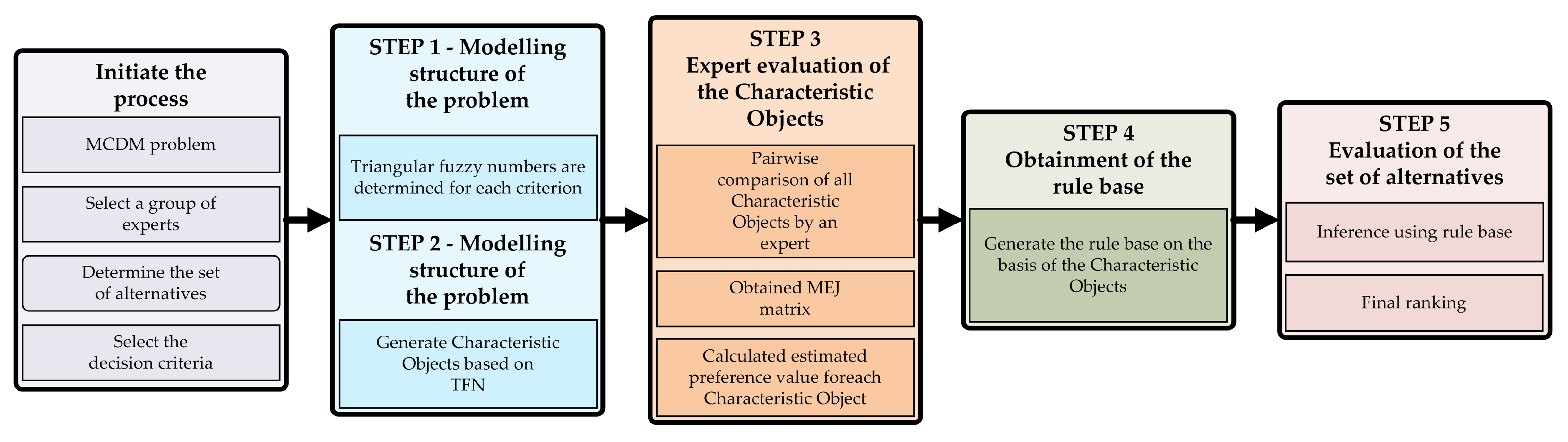
The whole decision-making process by using the COMET method is presented in Figure 1. The formal notation of this method can be presented using the following five steps [34]:

Step 1. Define the space of the problem – an expert determines dimensionality of the problem by selecting number r of criteria, $C_1,C_2,\dots ,C_r$. Subsequently, the set of fuzzy numbers for each criterion $C_i$ is selected, i.e., ${\tilde{C}}_{i1},{\tilde{C}}_{i2},\dots ,{\tilde{C}}_{i{c}_i}$. In this way, the following result is obtained:

$$\begin{array}{c}{C}_1=\{{\tilde{C}}_{11},{\tilde{C}}_{12},\dots ,{\tilde{C}}_{1c_1}\}\hfill \\ C_2=\{{\tilde{C}}_{21},{\tilde{C}}_{22},\dots ,{\tilde{C}}_{2c_1}\}\hfill \\ \dots \dots \dots \dots \dots \dots \dots \hfill \\ C_r=\{{\tilde{C}}_{r1},{\tilde{C}}_{r2},\dots ,{\tilde{C}}_{r{c}_r}\},\hfill \end{array}$$

(6)

where $c_1,c_2,\dots ,c_r$ are numbers of the fuzzy numbers for all criteria.

Step 2. Generate the characteristic objects—The characteristic objects ($CO$) are obtained by using the Cartesian Product of fuzzy numbers cores for each criteria as follows:

$$CO=C\left(C_1\right)\times C\left(C_2\right)\times \dots \times C\left(C_r\right).$$

(7)

As the result, the ordered set of all $CO$ is obtained:

$$\begin{array}{c}C{O}_1=C\left({\tilde{C}}_{11}\right),C\left({\tilde{C}}_{21}\right),\dots ,C\left({\tilde{C}}_{r1}\right)\hfill \\ C{O}_2=C\left({\tilde{C}}_{11}\right),C\left({\tilde{C}}_{21}\right),\dots ,C\left({\tilde{C}}_{r2}\right)\hfill \\ \dots \dots \dots \dots \dots \dots \dots \dots \dots \dots \dots \dots \hfill \\ C{O}_t=C\left({\tilde{C}}_{1c_1}\right),C\left({\tilde{C}}_{2c_2}\right),\dots ,C\left({\tilde{C}}_{r{c}_r}\right)\hfill \end{array},$$

(8)

where t is a number of $CO$:

$$t=\prod _{i=1}^r{c}_i.$$

(9)

Step 3. Rank the characteristic objects—the expert determines the Matrix of Expert Judgment ($MEJ$). It is a result of pairwise comparison of the characteristic objects by the expert knowledge. The $MEJ$ structure is as follows:

$$MEJ=\left(\begin{array}{cccc}{\alpha }_{11}& {\alpha }_{12}& \dots & {\alpha }_{1t}\\ {\alpha }_{21}& {\alpha }_{22}& \dots & {\alpha }_{2t}\\ \dots & \dots & \dots & \dots \\ {\alpha }_{t1}& {\alpha }_{t2}& \dots & {\alpha }_{tt}\end{array}\right),$$

(10)

where ${\alpha }_{ij}$ is a result of comparing $C{O}_i$ and $C{O}_j$ by the expert. The more preferred characteristic object gets one point and the second object get zero points. If the preferences are balanced, the both objects get half point. It depends solely on the knowledge of the expert and can be presented as:

$${\alpha }_{ij}=\{\begin{array}{cc}0.0,\hfill & f_{exp}\left(C{O}_i\right)<f_{exp}\left(C{O}_j\right)\hfill \\ 0.5,\hfill & f_{exp}\left(C{O}_i\right)=f_{exp}\left(C{O}_j\right)\hfill \\ 1.0,\hfill & f_{exp}\left(C{O}_i\right)>f_{exp}\left(C{O}_j\right)\hfill \end{array},$$

(11)

where $f_{exp}$ is an expert mental judgment function. Afterwards, the vertical vector of the Summed Judgments ($SJ$) is obtained as follows:

$$S{J}_i=\sum _{j=1}^t{\alpha }_{ij}.$$

(12)

The last step assigns to each characteristic object an approximate value of preference. In the result, the vector P is obtained, where $i$-th row contains the approximate value of preference for $C{O}_i$.

Step 4. The rule base—each characteristic object and value of preference is converted to a fuzzy rule as follows detailed form:

$$\begin{array}{cccccccc}IF\hfill & C\left({\tilde{C}}_{1i}\right)\hfill & AND\hfill & C\left({\tilde{C}}_{2i}\right)\hfill & AND\hfill & \dots \hfill & THEN\hfill & P_i\hfill \end{array}.$$

(13)

In this way, the complete fuzzy rule base is obtained, that approximates the expert mental judgement function $f_{exp}\left(C{O}_i\right)$

Step 5. Inference and final ranking—The each one alternative is a set of crisp numbers corresponding to criteria $C_1,C_2,\dots ,C_r$. It can be presented as follows:

$$A_i=\{a_{1i},a_{2i},\dots ,a_{ri}\}.$$

(14)

5. Results

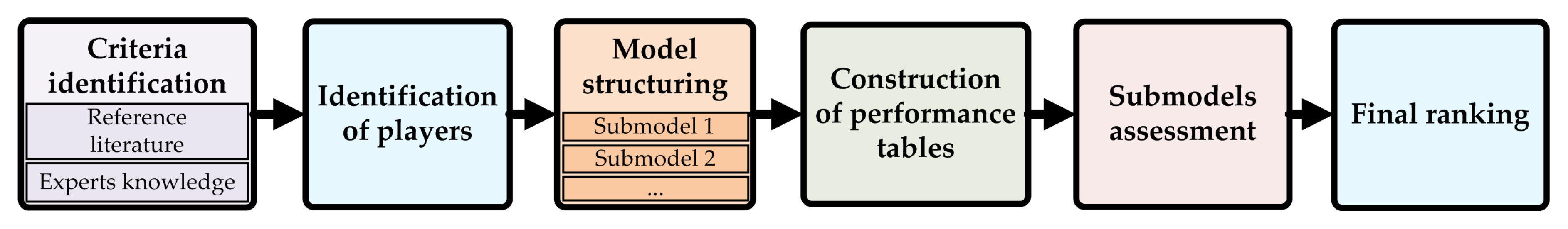
The detailed steps of the research to identify players carried out according to the methodical framework is presented in Figure 2. It is worth mentioning, once again, that algorithmic background and methodical approach provide COMET method.

The identified model creates a ranking, which is compared with Rating 2.0 that was proposed by Half-Life Television (HLTV). It is a news website that covers professional CS: GO news, tournaments, statistics, and rankings [23]. The obtained ranking is more natural to interpret. Each player assessment has three additional parameters. Many parameters influence the player’s performance, including the evaluation of his skills and predispositions. For instance, with player’s age, the drop-off in reaction time makes it hard for them to compete and harder to aim the head of moving target. High percentage of headshots reflects the shooting skills and is a kind of prestige [74]. There are plenty of criteria, which could be used to create an evaluation model. For instance, the damage per round given by grenades, the total number of rounds played by a player, which could inform us about the player’s experience or a high percentage of headshots, that was mentioned earlier. Other criteria have been chosen because of their greater impact on the assessment of the individual skills of each player. Especially important are the $C_1$ and $C_4$ criteria. They inform us that eliminating the player is smaller than the possibility that he will kill the enemies [74].

Many parameters influence the player’s performance, including the assessment of his skills and predispositions. For instance, with player’s age, the drop-off in reaction time makes it hard for them to compete and harder to aim the head of moving target. Hight percentage of headshots reflects the shooting skills and is a kind of prestige. Therefore, the following six criteria have been selected [22,23]:

• $C_1$—Average kills per round, the average number of kills scored by the player during one round;
• $C_2$—Average damage per round, mean damage inflicted by a player during one round;
• $C_3$—Total kills, the total number of kills gained by the player;
• $C_4$—K/D Ratio, the number of kills divided by number of deaths;
• $C_5$—Average assists per round, the mean number of assists gained by the player during one round; and
• $C_6$—Average deaths per round, the average number of deaths of a player during one round.

There are plenty of criteria, which could be used to create an evaluation model. For instance, the damage per round given by grenades, the total number of rounds played by a player, which could inform us about the player’s experience or a high percentage of headshots, that was mentioned earlier. However, a set of six criteria have been chosen because of their greater impact on the assessment of the individual skills of each player. The collected data for all applied criteria and Rating 2.0 assessment are derived from the official HLTV website and dated June 2019. Especially important are the $C_1$ and $C_4$ criteria. They inform us that the chance to eliminate the player is smaller than the possibility that he will kill the enemies.

The economy of a player depends on how much he has spent on weapons and armor, the kill awards that have been received per elimination (based on weapon type), the status of bomb planting or defusing, and finally who won the round [15]. Average kills per round ($C_1$) is always an important criterion because, by fragging (killing an enemy), you can eliminate first of all the threat from your opponent. For each elimination you get, depending on the weapon used, the amount of money needed to buy ammunition, equipment, grenades, and other utilities at a later stage of the game. For instance, elimination with a sniper rifle (AWP) is the least economically profitable and gives the player only USD 100, while almost any pistol gives 300 dollars reward, and shotguns, which are the most cost-effective, give even up to USD 900 in cash prize. Additionally, by killing enemies, they lose the weapons they acquired, thus losing all equipment, such as kevlar with a helmet or defuse kit (CT). Criterion $C_1$ is a profit type criterion, where the value increase means the preference increase. Based on the information about players statistics from the HLTV database for best 40 professional players, for $C_1$, the lowest obtained value is 0.72, the highest 0.88, and the average value is equal to 0.78.

As the number of Average damage per round increases, the probability of killing an enemy increases, as well. Moreover, the player is more priceless and useful for a team when he deprives the enemy team of the precious health points and makes gaining frag much easier for his teammates. There was a situation during the PGL Major Kraków 2017 event when a professional player Mikhail "Dosia" Stolyarov from Gambit Esports during the grand final against Immortals team done some unbelievable action. His team (on CT side) was going to lose the round because there was not enough time to defuse the bomb versus three opponents. Dosia knew it was impossible to win, but he came up with an idea and threw a grenade to give some extra damage to players, who were saving their weapons. It was a few seconds before the detonation of the bomb, which takes many health points (HP) from players located in an area of the explosion. Doing it, he contributed to the death of two players, which lost precious weapons and equipment, forcing them to spent extra money in the next round. That was an example of the validity of this criterion on the professional field of CS: GO. Criterion $C_2$ is characterized by a positive correlation to player value. For criterion $C_2$, the lowest result is 75.60, the highest 88.20, and the mean value is equal to 82.70.

Criterion $C_3$ determine the total number of kills scored by the player, which could signify that the player plays a lot and has a background in Counter-Strike, like the legendary player Christopher “GeT RiGhT” Alesund from Sweden or Filip “Neo” Kubski from Poland. When $C_3$ value increases, the player’s evaluation also improves. As the total number of kills increases, the player’s skill level and overall experience develop, as well, playing later against much better enemies. For criterion $C_3$, the lowest result is 1516.00, the highest 4151.00, and the mean value is equal to 2514.90. Frankly, it is not the most critical parameter because players with much less number of frags could play as good or even better. It depends on individual predispositions and the innate potential of the gamer.

Criterion $C_4$ is probably the most prominent rate of players’ abilities in CS: GO. It is a profit type criterion, like the previous three criteria. It informs us that the chance to eliminate the player is smaller than the possibility that he will kill the enemies. If the total number of kills is more significant than the overall number of deaths, the player’s skill level is getting more superior, and the gamer improves every time he plays. For professional gamers, the criterion $C_4$ obtained the lowest result equal to 1.15, the highest 1.51, and the mean value is equal to 1.25. Even the worst K/D Ratio value in this set of players is a great result.

Obtaining assistance in team games is proof of successful and productive team play. In CS: GO, assists are also received in this way because it is an evident proof that the player was close to making an elimination on the opponent. However, something went wrong and only deprived him of most of the health points in the end without gaining a single frag. Then, he gives his teammates the opportunity for an easy kill, but he only got an assist instead of a full frag on his account. Often, players who play a supporting role get a significant amount of assists because they contribute to getting eliminations on the rival by, for example, blinding him with a flashlight, helping his colleagues. For criterion $C_5$, the lowest result is 0.09, the highest 0.18, and the average value is equal to 0.13.

As it is known in FPS games, the most important thing is to eliminate your opponents instead of being killed. By analyzing the Average number of deaths per round, we can conclude which player loses the most shooting duels and has to observe the actions of his teammates only as an observer. It could show us the weakness of the player and skill shortages that will allow the best ones to be distinguished. It is a cost-type criterion, which means the value increase indicates the preference decrease. For criterion $C_6$, the lowest result is 0.52, the highest 0.68, and the mean value is equal to 0.63.

The values of selected criteria $C_1$–$C_6$, positions and names of alternatives are presented in the

Table 2. The performance table of the alternatives and selected criteria.

Pos.	Name	${\mathit{C}}_1$	${\mathit{C}}_2$	${\mathit{C}}_3$	${\mathit{C}}_4$	${\mathit{C}}_5$	${\mathit{C}}_6$
1	s1mple	0.88	86.6	1958	1.50	0.09	0.59
2	ZywOo	0.83	85.3	4151	1.40	0.12	0.59
3	Jame	0.78	79.3	3505	1.51	0.09	0.52
4	Jamppi	0.83	83.1	2851	1.30	0.1	0.64
5	huNter	0.80	88.2	4100	1.22	0.15	0.66
6	vsm	0.80	86.6	2420	1.22	0.13	0.65
7	meyern	0.82	83.8	1728	1.28	0.12	0.64
8	Kaze	0.78	80.7	1750	1.32	0.1	0.60
9	Hatz	0.76	81.8	2017	1.28	0.15	0.60
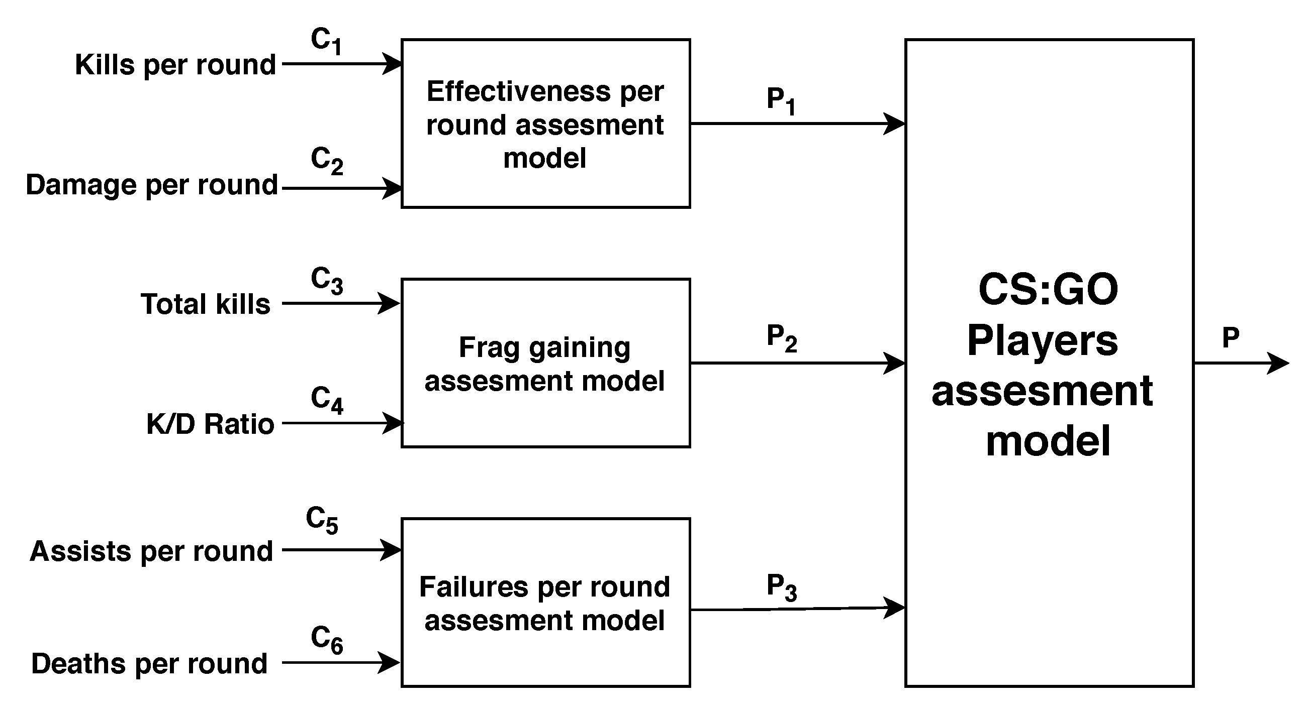
10	Sico	0.76	78.4	1876	1.36	0.13	0.56

. In this study case, the considered problem is simplified to a structure, which is presented in Figure 3.

In that way, we have to identify three related models, where each one requires a lot smaller number of queries to the expert. The final decision model consists of three following models, where, for each one, nine characteristic objects and 36 pairwise comparisons are needed:

• $P_1$—Effectiveness per round assessment model with two inputs;
• $P_2$—Frag gaining assessment model with two inputs;
• $P_3$—Failures per round assessment model with two inputs.

In the Effectiveness per round assessment model ($P_1$), we aggregate two essential criteria, like Average kills per round ($C_1$) and Average damage per round ($C_2$), as input values. The output value is our player evaluation for model $P_1$, and the lowest result is 0.23, the highest 0.88, and the mean value is equal to 0.45 for top 40 professional players in CS: GO. The input values of the Frag gaining assessment model ($P_2$) are two significant criteria, like Total kills ($C_3$) and K/D Ratio ($C_4$). The outcome value is our player assessment for model $P_2$, and the lowest result is 0.00, the highest 0.84, and the mean value is equal to 0.45. In the Failures per round assessment model ($P_3$), we connect two crucial criteria, like Average assists per round ($C_5$) and Average deaths per round ($C_6$). The output value is our player evaluation for model $P_3$, and the lowest result is 0.25, the highest 0.78, and the mean value is equal to 0.44.

The model will be validated based on the results obtained from the official HLTV website for the top 10 professional CS: GO players for June 2019, which are presented in Table 2. To identify the final model for players assessment, we have to determine the three following assessment models, i.e., Effectiveness per round, Frag gaining, and Failures per round.

5.1. Effectiveness per Round Assessment Model

This model evaluates the efficiency in eliminating and injuring enemies, which is one of the essential elements of CS: GO. The expert identified two significant criteria for the Effectiveness per round assessment model: Average kills per round, which is the mean number of frags scored by the player pending one round, and Average damage per round, that is mean damage delivered by a player during one round. Both of them are a profit type criteria, where the value increase means the preference increase. In such complex problems, the relationship is sporadically linear.

Table 3. Overview of characteristic objects $CO$, vector P values for the Effectiveness per round assessment model.

${\mathit{CO}}_{\mathit{i}}$	${\mathit{C}}_1$	${\mathit{C}}_2$	${\mathit{P}}_1$
$C{O}_1$	0.7	70	0.0000
$C{O}_2$	0.7	80	0.1250
$C{O}_3$	0.7	90	0.2500
$C{O}_4$	0.8	70	0.3750
$C{O}_5$	0.8	80	0.5000
$C{O}_6$	0.8	90	0.6250
$C{O}_7$	0.9	70	0.7500
$C{O}_8$	0.9	80	0.8750
$C{O}_9$	0.9	90	1.0000

presents the values of the criteria $C_1$ and $C_2$ and the $P_1$ assessment model. Based on the presented data, it can be determined that the best value of the criteria $C_1$ was achieved by ‘Simple’, which is equal to 0.88, while the worst result was obtained by ‘dexter’ with the value equal to 0.72. In the case of the second criterion, the best score was given to ‘huNter’ with 88.2, and the lowest score was received by ‘xsepower’ with value equal to 75.6. 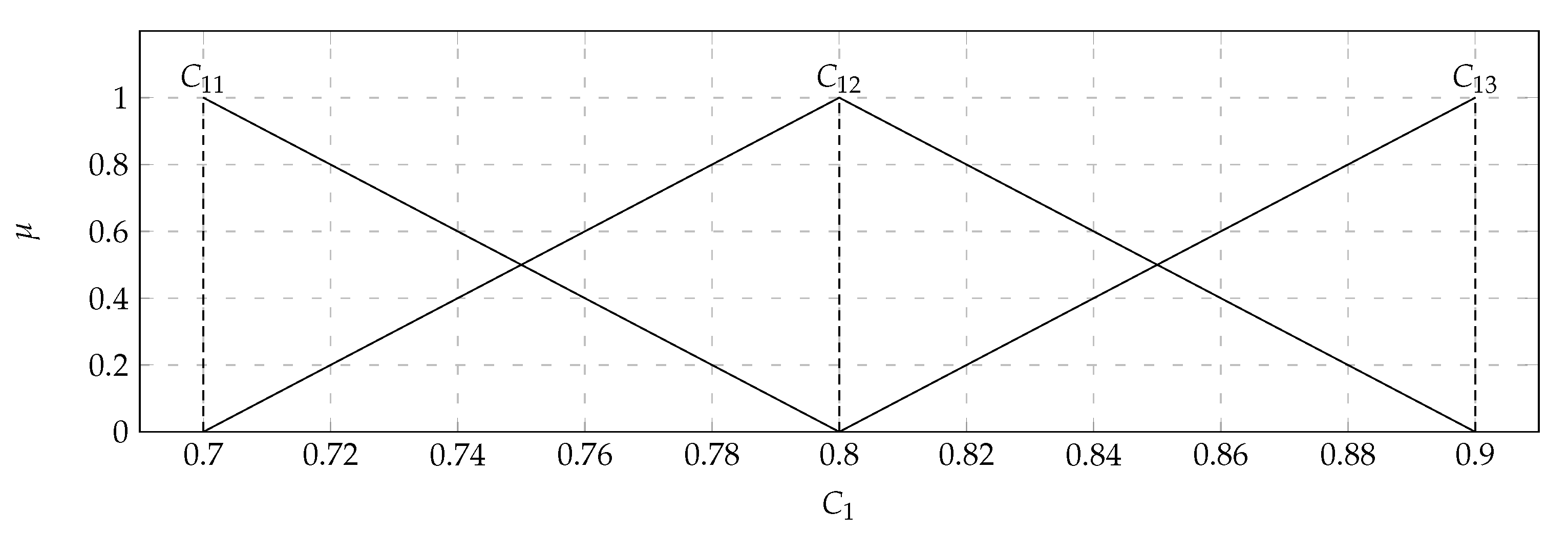Analyzing the results of the effectiveness per round assessment model ($P_1$), we can conclude that the highest score $P_1$ was obtained by ‘Simple’, and is equal to 0.8825. The triangular fuzzy numbers of criterium $C_1$ are presented in Figure 4, while $C_2$ is presented in Figure 5.

In the considered set of parameters, there were players with: Average kills per round ($C_1$) with the values of the support of the triangular fuzzy number from 0.7 ($C_{11}$) to 0.9 ($C_{13}$) and the core valued 0.8 ($C_{12}$); Average damage per round ($C_2$) with the values of the support of the triangular fuzzy number from 70 ($C_{21}$) to 90 ($C_{23}$) and the core valued 0.8 ($C_{22}$) health points. Based on the data presented in the

Table 4. The performance table of the selected criteria $C_1$, $C_2$ and assessment model $P_1$.

Pos.	Name	${\mathit{C}}_1$	${\mathit{C}}_2$	${\mathit{P}}_1$
1	s1mple	0.88	86.6	0.8825
2	ZywOo	0.83	85.3	0.6788
3	Jame	0.78	79.3	0.4163
4	Jamppi	0.83	83.1	0.6513
5	huNter	0.80	88.2	0.6025
6	vsm	0.80	86.6	0.5825
7	meyern	0.82	83.8	0.6225
8	Kaze	0.78	80.7	0.4338
9	Hatz	0.76	81.8	0.3725
10	Sico	0.76	78.4	0.3300

, it turned out that the output $P_1$ takes values from 0.1 to 0.9. Therefore, the variable $P_1$ will take two values. Both of them will also be determined as triangular fuzzy numbers. They were displayed in Figure 6. The comparison of the 36 pairwise of the 9 characteristic objects were executed. Consequently, the Matrix of Expert Judgment ($MEJ$) was defined as (15), where each ${\alpha }_{ij}$ value was calculated using Equation (11).

$$MEJ=\left(\begin{array}{ccccccccc}0.5& 0& 0& 0& 0& 0& 0& 0& 0\\ 1& 0.5& 0& 0& 0& 0& 0& 0& 0\\ 1& 1& 0.5& 0& 0& 0& 0& 0& 0\\ 1& 1& 1& 0.5& 0& 0& 0& 0& 0\\ 1& 1& 1& 1& 0.5& 0& 0& 0& 0\\ 1& 1& 1& 1& 1& 0.5& 0& 0& 0\\ 1& 1& 1& 1& 1& 1& 0.5& 0& 0\\ 1& 1& 1& 1& 1& 1& 1& 0.5& 0\\ 1& 1& 1& 1& 1& 1& 1& 1& 0.5\end{array}\right).$$

(15)

As a result, the vector of the Summed Judgements ($SJ$) was calculated using Equation (12), and it was employed to determine the values of preference ($P_1$), which are presented in Table 3. The characteristic objects $C{O}_1$–$C{O}_9$ presented in Table 3 are generated using the Cartesian product of the fuzzy numbers’ cores of criteria $C_1$ and $C_2$. The highest value of preference $P_1$ received $C{O}_9$ with a triangular fuzzy number of criterion $C_1$ valued 0.9 ($C_{13}$) and with a triangular fuzzy number of criterion $C_2$ valued 90 ($C_{23}$). The lowest value of preference $P_1$ fell to $C{O}_1$ with a triangular fuzzy number of criterion $C_1$ valued 0.7 ($C_{11}$) and with a triangular fuzzy number of criterion $C_2$ valued 70 ($C_{21}$). With an increase in the value of the criterion $C_1$, the preference increases more significantly than with an increase in the value of the criterion $C_2$. It means that $C_1$ has a greater impact on the assessment of the $P_1$ model than $C_2$.

For a better demonstration of the relevance of the criteria to the $P_1$ assessment model, a $\rho$ Spearman’s rank correlation coefficient was calculated. $\rho$ Spearman’s rank correlation coefficient between the criteria $C_1$, $C_2$ and reference ranking obtained by $P_1$ assessment model for top 10 players is equal to 0.9273 and 0.2970. The correlation between the first one is strong, while, in the second one, it is weak. The visualization of the relation diagram of Average kills per round ($C_1$) and $P_1$ assessment model, as well as the relation diagram of Average damage per round ($C_2$) and $P_1$ assessment model, is presented in Figure 7.

5.2. Frag Gaining Assessment Model

The model verifies the probability of a player to get an elimination based on the number of kills he has obtained in official CS: GO matches and a specific factor, which shows that the player is superior. The expert identified two significant criteria for the Frag gaining assessment model. Total kills, which is the total number of frags delivered by the player, and K/D Ratio, that is the number of frags divided by the number of deaths. Both of them are profit type criteria, whereas it was mentioned earlier, with the increase in values, preference increases, too.

Table 5. Overview of characteristic objects $CO$, vector P values for the Frag gaining assessment model.

${\mathit{CO}}_{\mathit{i}}$	${\mathit{C}}_3$	${\mathit{C}}_4$	${\mathit{P}}_2$
$C{O}_1$	0	1.0	0.0000
$C{O}_2$	0	1.25	0.3750
$C{O}_3$	0	1.6	0.7500
$C{O}_4$	0.5	1.0	0.1250
$C{O}_5$	0.5	1.25	0.5000
$C{O}_6$	0.5	1.6	0.8750
$C{O}_7$	1.0	1.0	0.2500
$C{O}_8$	1.0	1.25	0.6250
$C{O}_9$	1.0	1.6	1.0000

shows the values of the criteria $C_3$ and $C_4$ and the $P_2$ assessment model. Based on the presented data, it can be determined that the best value of the criteria $C_3$ was achieved by ‘ZywOo’, which is equal to 1.000, while the worst result was obtained by ‘BnTeT’ with the value equal to 0. In the case of the second criterion, the best score was given to ‘Jame’ with 1.51, and the lowest score was received by ‘Texta’ with a value equal to 1.15. Analyzing the results of the Frag gaining assessment model ($P_2$), we can conclude that the highest score was obtained by ‘Jame’, and is equal to 0.8423. The triangular fuzzy numbers of criterium $C_3$ are presented in Figure 8 and $C_4$ in Figure 9.

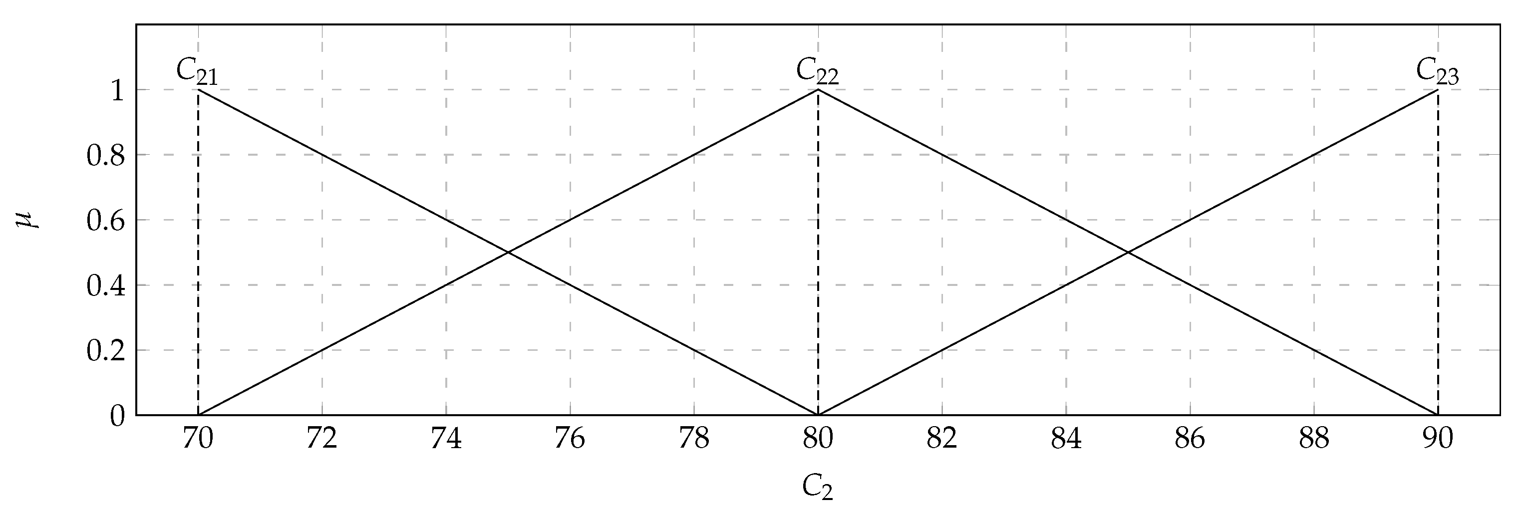
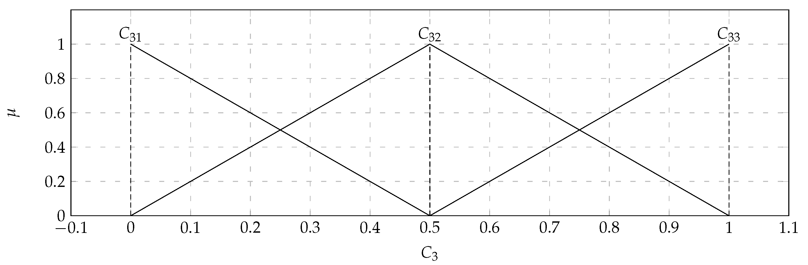
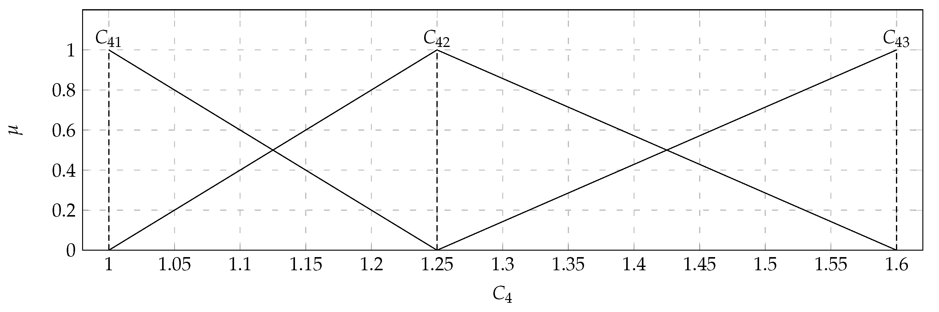
In the considered set of parameters, there were players with: total kills ($C_3$) with the values of the support of the triangular fuzzy number from 0 ($C_{31}$) to 1 ($C_{33}$) and the core valued 0.5 ($C_{32}$); K/D ratio ($C_4$) with the values of the support of the triangular fuzzy number from 1 ($C_{41}$) to 1.6 ($C_{43}$) and the core valued 1.25 ($C_{42}$). Based on the data presented in the

Table 6. The performance table of the selected criteria $C_3$, $C_4$ and assessment model $P_2$.

Pos.	Name	${\mathit{C}}_3$	${\mathit{C}}_4$	${\mathit{P}}_2$
1	s1mple	0.168	1.50	0.6849
2	ZywOo	1.000	1.40	0.7857
3	Jame	0.755	1.51	0.8423
4	Jamppi	0.507	1.30	0.5553
5	huNter	0.981	1.22	0.5753
6	vsm	0.343	1.22	0.4158
7	meyern	0.080	1.28	0.4271
8	Kaze	0.089	1.32	0.4723
9	Hatz	0.190	1.28	0.4546
10	Sico	0.137	1.36	0.5271

, it turned out that the output $P_2$ takes values from 0.2 to 0.9. Therefore, the variable $P_2$ will take two values. Both of them will also be saved as triangular fuzzy numbers. They are displayed in Figure 10. The comparison of the 36 pairwise of the 9 characteristic objects was executed. Consequently, the Matrix of Expert Judgment ($MEJ$) was defined (16), where each ${\alpha }_{ij}$ value was calculated using Equation (11).

$$MEJ=\left(\begin{array}{ccccccccc}0.5& 0& 0& 0& 0& 0& 0& 0& 0\\ 1& 0.5& 0& 1& 0& 0& 1& 0& 0\\ 1& 1& 0.5& 1& 1& 0& 1& 1& 0\\ 1& 0& 0& 0.5& 0& 0& 0& 0& 0\\ 1& 1& 0& 1& 0.5& 0& 1& 0& 0\\ 1& 1& 1& 1& 1& 0.5& 1& 1& 0\\ 1& 0& 0& 1& 0& 0& 0.5& 0& 0\\ 1& 1& 0& 1& 1& 0& 1& 0.5& 0\\ 1& 1& 1& 1& 1& 1& 1& 1& 0.5\end{array}\right).$$

(16)

As a result, the vector of the Summed Judgements ($SJ$) was calculated using Equation (12), and it was used to determine the values of preference ($P_2$), which are presented in Table 5. The characteristic objects $C{O}_1$–$C{O}_9$ presented in Table 5 are generated using the Cartesian product of the fuzzy numbers’ cores of criteria $C_3$ and $C_4$. The highest value of preference $P_2$ received $C{O}_9$ with a triangular fuzzy number of criterion $C_3$ valued 1 ($C_{33}$) and with a triangular fuzzy number of criterion $C_4$ valued 1.6 ($C_{43}$). The lowest value of preference $P_2$ fell to $C{O}_1$ with a triangular fuzzy number of criterion $C_3$ valued 0 ($C_{31}$) and with a triangular fuzzy number of criterion $C_4$ valued 1 ($C_{41}$). With an increase in the value of the criterion $C_4$, the preference increases more significantly than with an increase in the value of the criterion $C_3$. It means that $C_4$ has a greater impact on the assessment of the $P_2$ model than $C_3$.

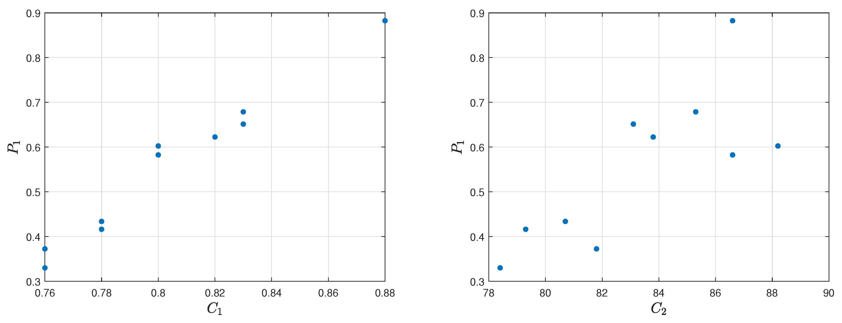
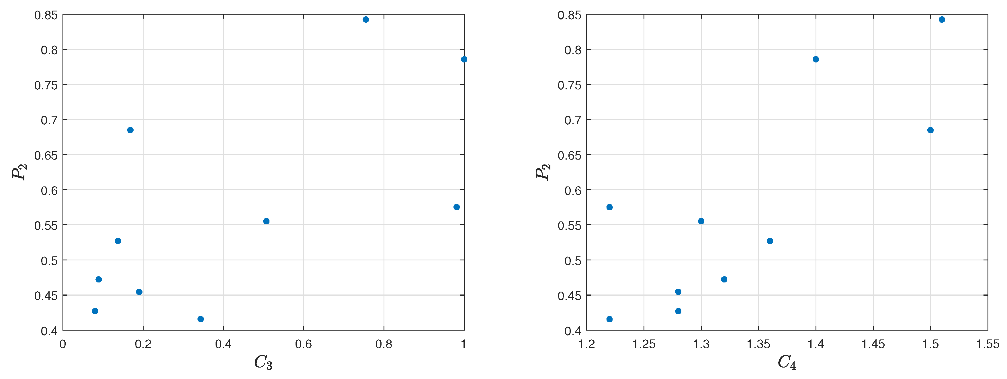
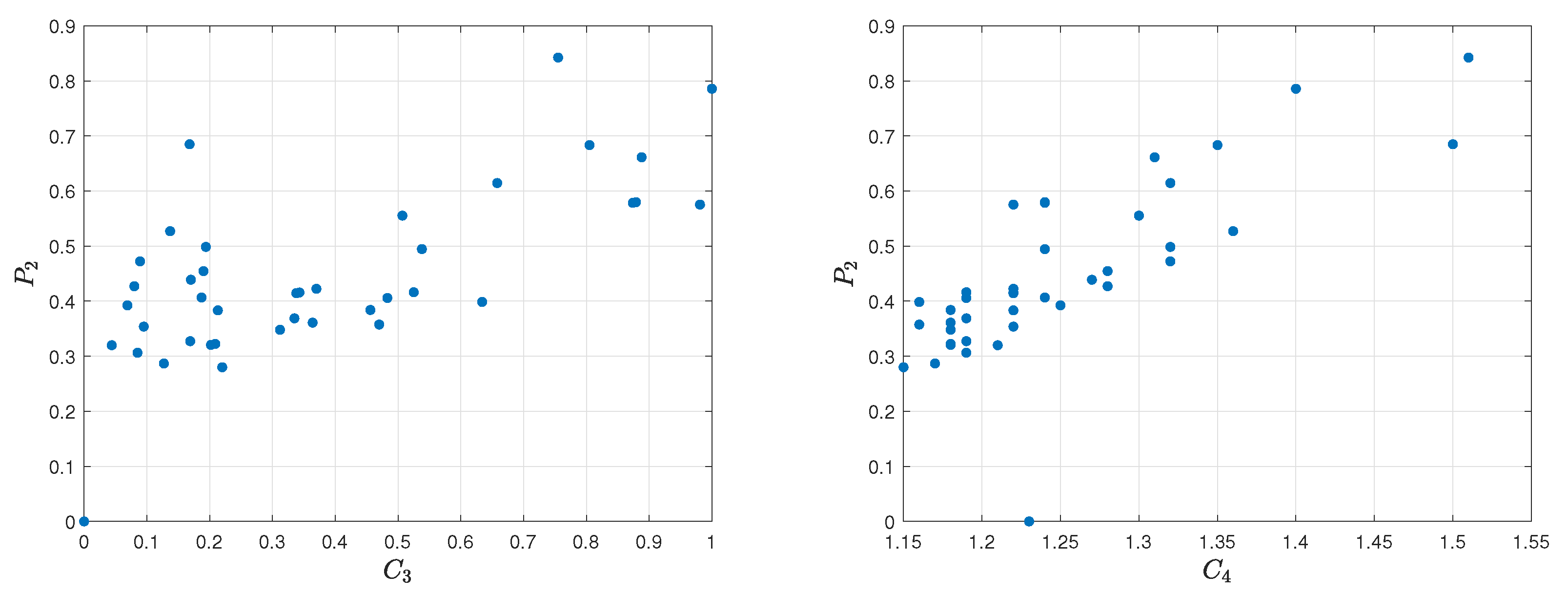
For a better demonstration of the relevance of the criteria to the $P_2$ assessment model, a $\rho$ Spearman’s rank correlation coefficient was calculated. $\rho$ Spearman’s rank correlation coefficient between the criteria $C_3$, $C_4$, and reference ranking obtained by $P_2$ assessment model is equal to 0.5636 and 0.4910. The correlation between the first one and the reference ranking is moderately strong, while, in the second one, it is weak. The visualization of the relation diagram of total kills ($C_3$) and $P_2$ assessment model, as well as the relation diagram of K/D ratio ($C_4$) and $P_1$ assessment model, is shown in Figure 11.

5.3. Failures per Round Assessment Model

This model evaluates the weaker side of the player by showing how often he has a decline in form and skill deficiencies, which are vital to maintaining himself at the top of the global e-sport scene. The expert identified two crucial criteria for the Failures per round assessment model. Average assists per round, which is the average number of assists scored by the player during one round and Average deaths per round, that is the average number of deaths of a player pending one round. The first one is a profit type criterion, which means that the value increase indicates the preference increase; however, the second one is a cost-type criterion, which means the value increase indicates the preference decrease.

Table 7. Overview of characteristic objects $CO$, vector P values for the Failures per round assessment model.

${\mathit{CO}}_{\mathit{i}}$	${\mathit{C}}_5$	${\mathit{C}}_6$	${\mathit{P}}_3$
$C{O}_1$	0.05	0.5	0.7500
$C{O}_2$	0.1	0.5	0.8750
$C{O}_3$	0.2	0.5	1.0000
$C{O}_4$	0.05	0.6	0.3750
$C{O}_5$	0.1	0.6	0.5000
$C{O}_6$	0.2	0.6	0.6250
$C{O}_7$	0.05	0.7	0.0000
$C{O}_8$	0.1	0.7	0.1250
$C{O}_9$	0.2	0.7	0.2500

shows the values of the criteria $C_5$ and $C_6$ and the $P_3$ assessment model. Based on the presented data, it can be determined that the best value of the criteria $C_5$ was achieved by ‘INS’, which is equal to 1.18, while the worst result was obtained by ‘kNgV-’ with the value equal to 0.09. In the case of the second criterion, the best score was given to ‘Jame’ with 0.52, and the worst score was received by ‘roeJ’ with a value equal to 0.68. Analyzing the results of the Failures per round assessment model ($P_3$), we can conclude that the highest score was obtained by ‘Jame’ and is equal to 0.7750. The triangular fuzzy numbers of criterium $C_5$ are presented in Figure 12 and $C_6$ in Figure 13.

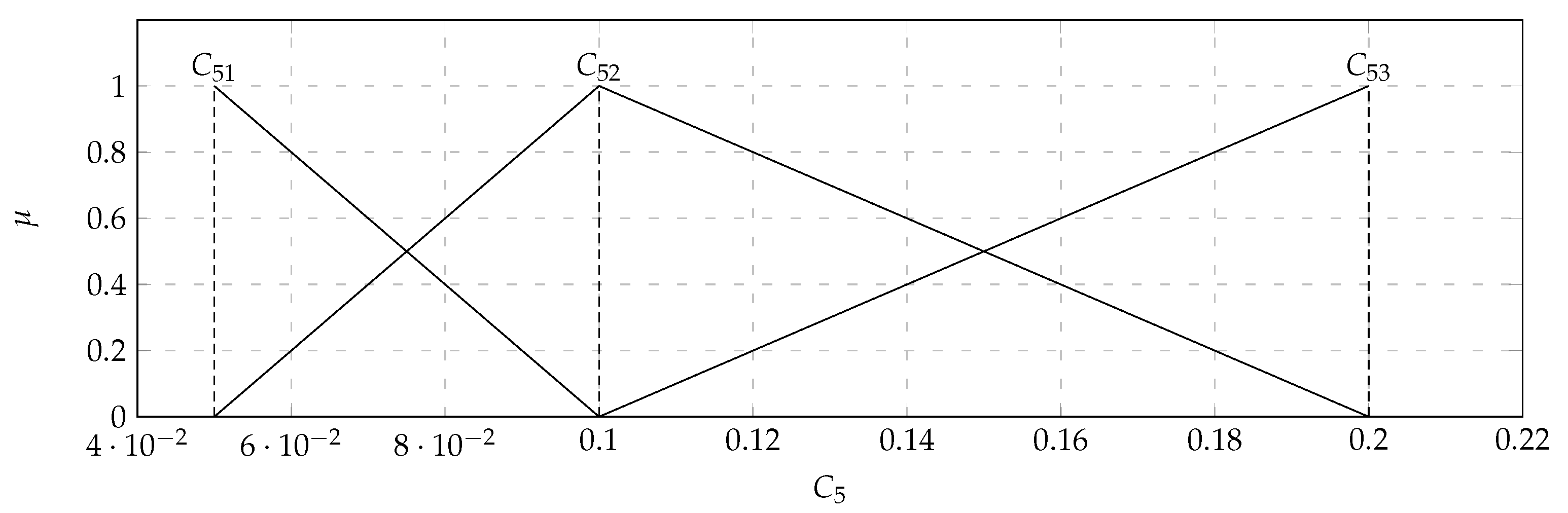
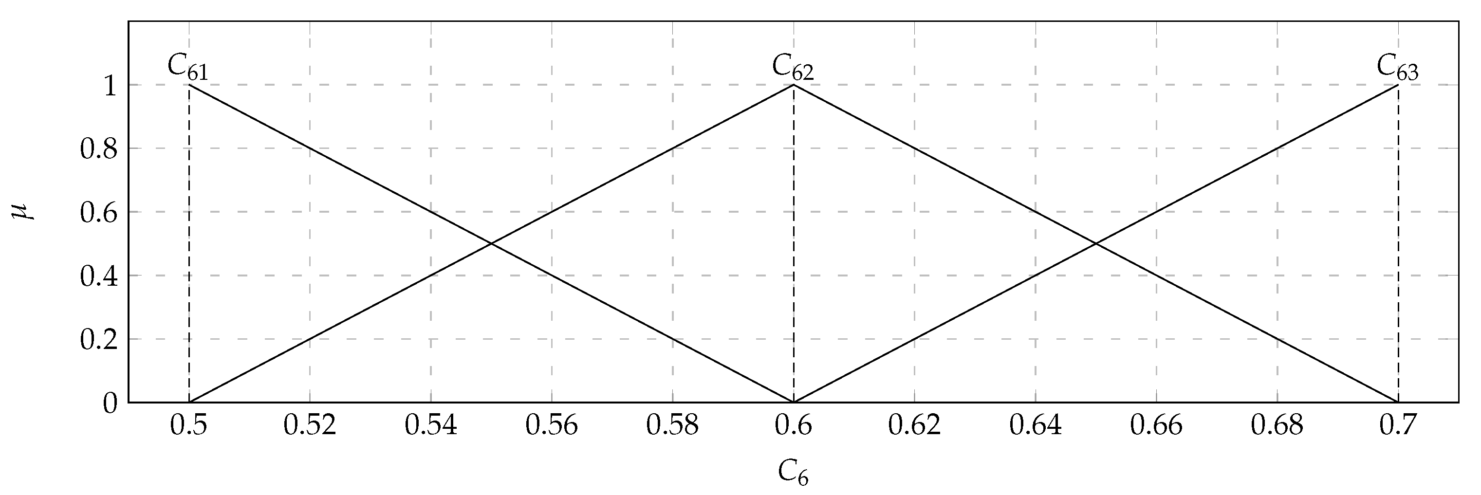
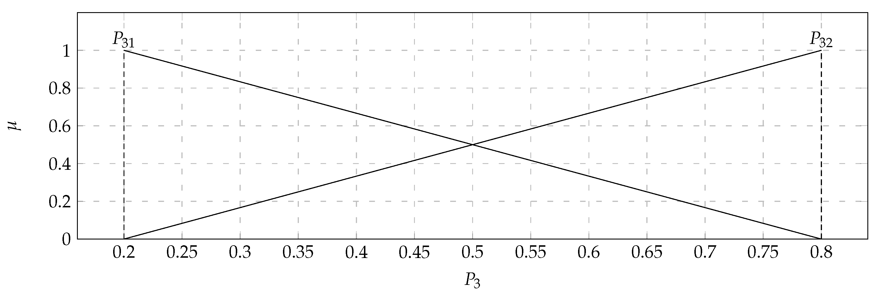
In the considered set of parameters there were players with: Average assists per round ($C_5$) with the values of the support of the triangular fuzzy number from 0.05 ($C_{51}$) to 0.2 ($C_{53}$) and the core valued 0.1 ($C_{52}$); Average deaths per round ($C_6$) with the values of the support of the triangular fuzzy number from 0.5 ($C_{61}$) to 0.7 ($C_{63}$) and the core valued 0.6 ($C_{62}$). Based on the data presented in the

Table 8. The performance table of the selected criteria $C_5$, $C_6$ and assessment model $P_3$.

Pos.	Name	${\mathit{C}}_5$	${\mathit{C}}_6$	${\mathit{P}}_3$
1	s1mple	0.09	0.59	0.5125
2	ZywOo	0.12	0.59	0.5625
3	Jame	0.09	0.52	0.7750
4	Jamppi	0.10	0.64	0.3500
5	huNter	0.15	0.66	0.3375
6	vsm	0.13	0.65	0.3500
7	meyern	0.12	0.64	0.3750
8	Kaze	0.10	0.60	0.5000
9	Hatz	0.15	0.60	0.5625
10	Sico	0.13	0.56	0.6875

, it turned out that the output $P_3$ takes values from 0.2 to 0.8. Therefore, the variable $P_3$ will take two values. Both of them will also be saved as triangular fuzzy numbers. They were displayed in Figure 14. The comparison of the 36 pairwise of the 9 characteristic objects were executed. Consequently, the Matrix of Expert Judgment ($MEJ$) was defined (17), where each ${\alpha }_{ij}$ value was calculated using Equation (11).

$$MEJ=\left(\begin{array}{ccccccccc}0.5& 0& 0& 1& 1& 1& 1& 1& 1\\ 1& 0.5& 0& 1& 1& 1& 1& 1& 1\\ 1& 1& 0.5& 1& 1& 1& 1& 1& 1\\ 0& 0& 0& 0.5& 0& 0& 1& 1& 1\\ 0& 0& 0& 1& 0.5& 0& 1& 1& 1\\ 0& 0& 0& 1& 1& 0.5& 1& 1& 1\\ 0& 0& 0& 0& 0& 0& 0.5& 0& 0\\ 0& 0& 0& 0& 0& 0& 1& 0.5& 0\\ 0& 0& 0& 0& 0& 1& 1& 0& 0.5\end{array}\right).$$

(17)

As a result, the vector of the Summed Judgements ($SJ$) was calculated using Equation (12), and it was employed to determine the values of preference ($P_3$), which are presented in Table 7. The characteristic objects $C{O}_1$–$C{O}_9$ presented in Table 7 are generated using the Cartesian product of the fuzzy numbers’ cores of criteria $C_5$ and $C_6$. The highest value of preference $P_3$ received $C{O}_3$ with a triangular fuzzy number of criterion $C_5$ valued 0.2 ($C_{53}$) and with a triangular fuzzy number of criterion $C_6$ valued 0.5 ($C_{63}$). The lowest value of preference $P_3$ fell to $C{O}_7$ with a triangular fuzzy number of criterion $C_5$ valued 0.05 ($C_{51}$) and with a triangular fuzzy number of criterion $C_6$ valued 0.7 ($C_{61}$). With a decrease in the value of the criterion $C_6$, the preference increases more significantly than with an increase in the value of the criterion $C_5$. It means that $C_6$ has a greater impact on the assessment of the $P_3$ model than $C_5$.

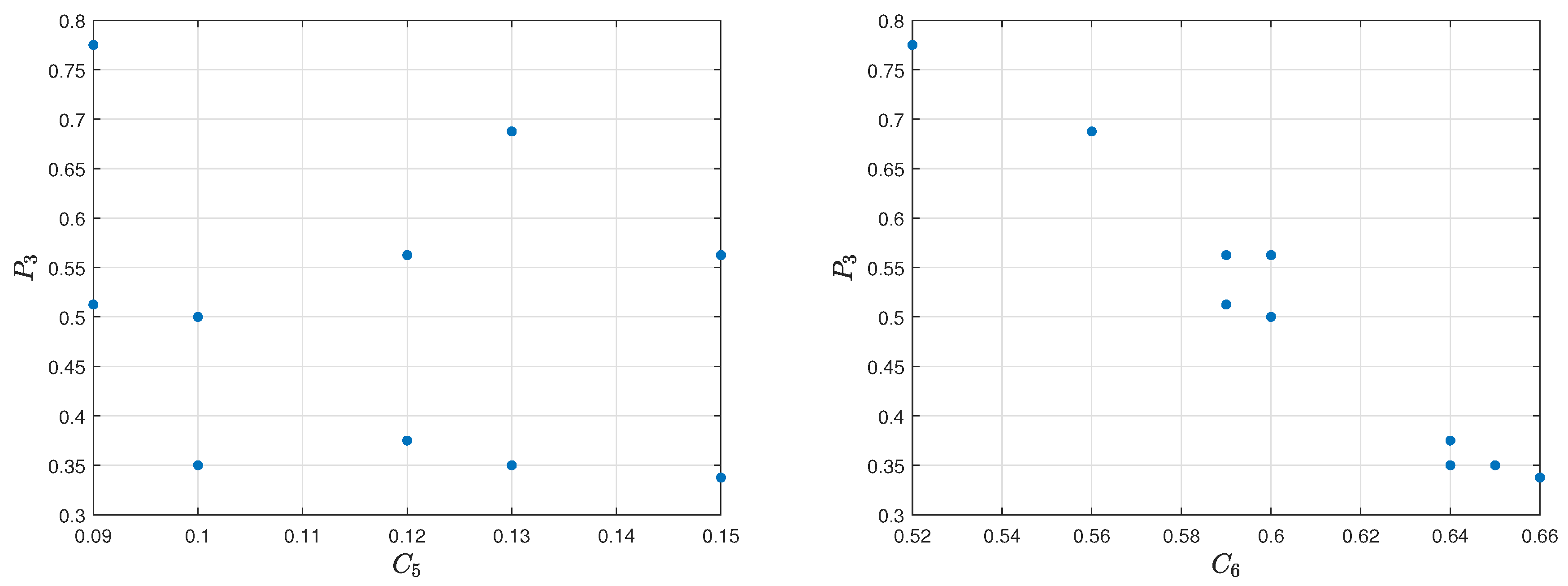
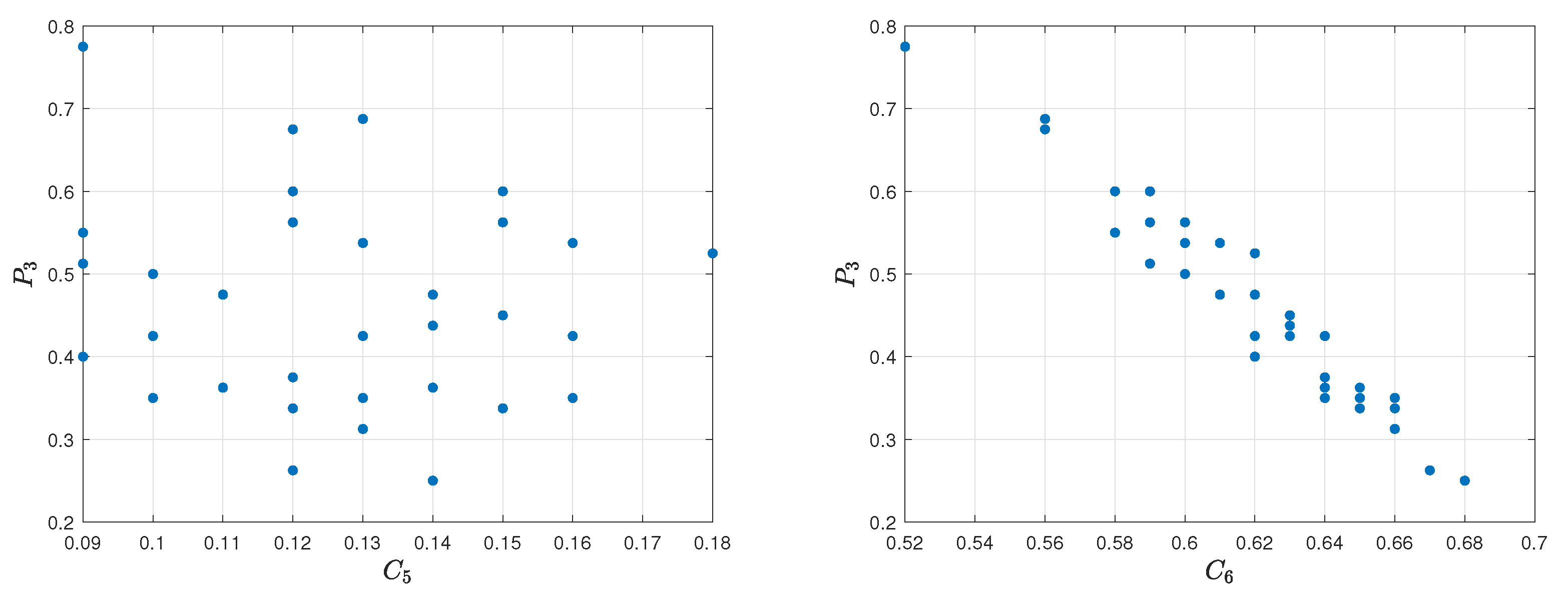
For a better demonstration of the relevance of the criteria to the $P_3$ assessment model, a $\rho$ Spearman’s rank correlation coefficient was calculated. $\rho$ Spearman’s rank correlation coefficient between the criteria $C_5$, $C_6$, and reference ranking obtained by $P_3$ assessment model is equal to 0.5273 and 0.1636. The correlation between the first one and the reference ranking is moderately strong, while, in the second one, it is weak. The visualization of the relation diagram of Average assists per round ($C_5$) and $P_3$ assessment model, as well as the relation diagram of Average deaths per round ($C_6$) and $P_3$ assessment model, is shown in Figure 15.

5.4. Final Model

CS: GO Players assessment model finally determines the uniqueness of the Counter-Strike Global: Offensive player by placing him in the final ranking, based on previous partial assessments. The final model for the players’ assessment has three aggregated input variables. The output variable from the Effectiveness per round assessment, Frag gaining assessment, and the output variable from the Failures per round assessment were applied. The aggregated variables $P_1$ and $P_2$ are both profit type, whereas the $P_3$ is cost type. The triangular fuzzy numbers of parameter $P_1$ is presented in Figure 16, $P_2$ in Figure 17, and $P_3$ in Figure 18.

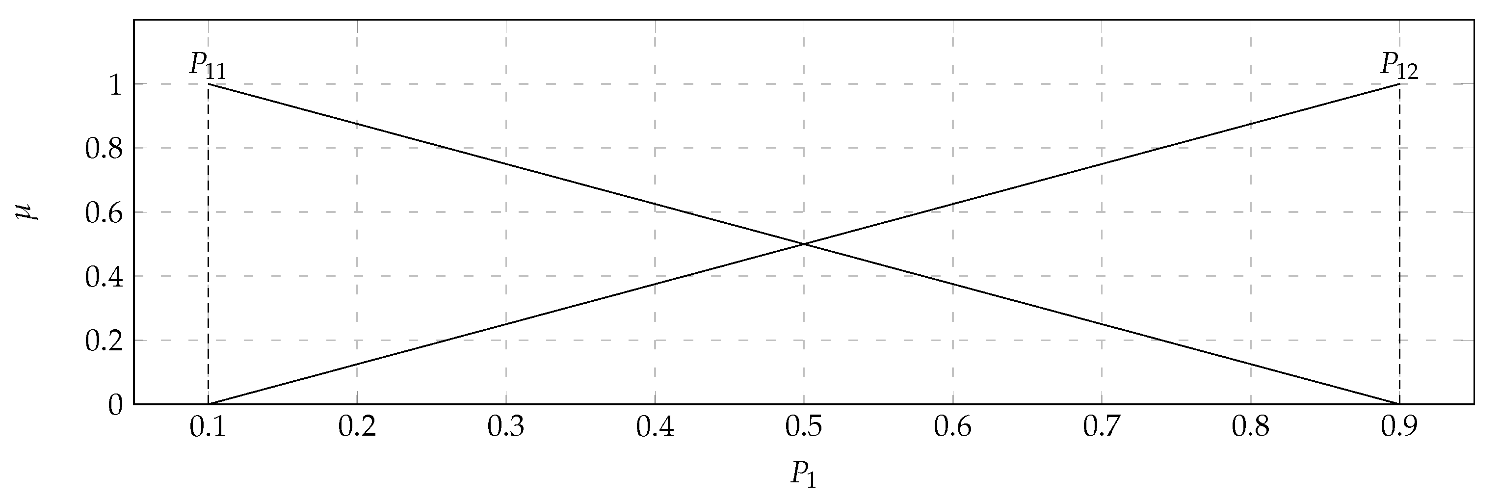
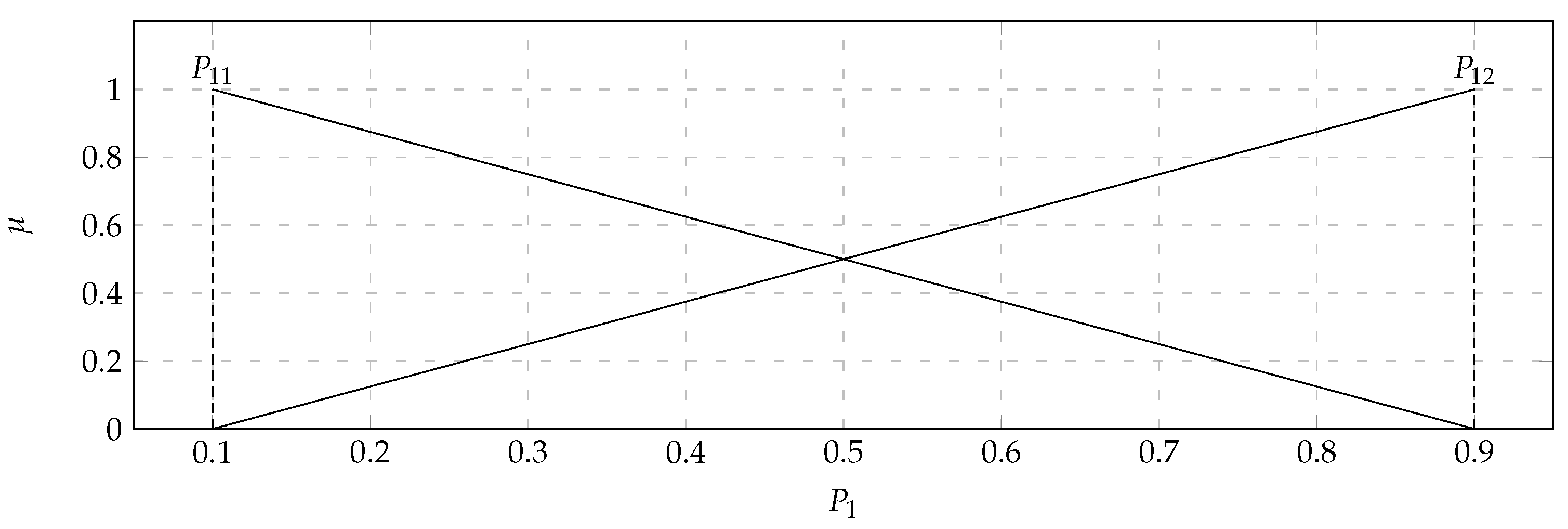
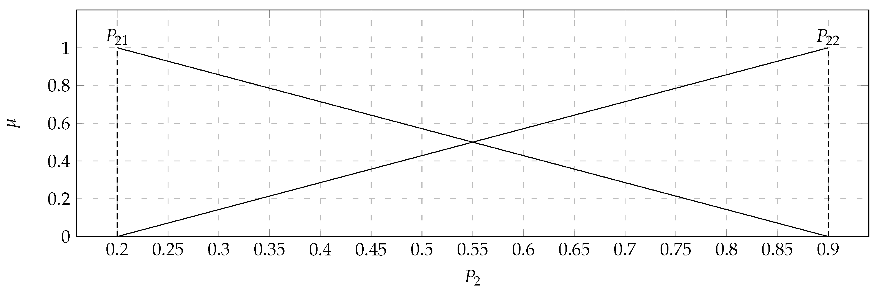
In the considered set of parameters there were players with: Effectiveness per round ($P_1$) with the values of the support of the triangular fuzzy number from 0.2 ($P_{11}$) to 1 ($P_{12}$), Frag gaining ($P_2$) with the values of the support of the triangular fuzzy number from 0.1 ($P_{21}$) to 0.9 ($P_{22}$), Failures per round ($P_3$) with the values of the support of the triangular fuzzy number from 0.2 ($P_{31}$) to 0.9 ($P_{32}$). The comparison of the 28 pairwise of the 8 characteristic objects were executed. Consequently, the Matrix of Expert Judgment ($MEJ$) was defined as (18), where each ${\alpha }_{ij}$ value was calculated using Equation (11).

$$MEJ=\left(\begin{array}{cccccccc}0.5& 0& 0& 0& 1& 0& 0& 0\\ 1& 0.5& 1& 0& 1& 1& 1& 0\\ 1& 0& 0.5& 0& 1& 0& 1& 0\\ 1& 1& 1& 0.5& 1& 1& 1& 1\\ 0& 0& 0& 0& 0.5& 0& 0& 0\\ 1& 0& 1& 0& 1& 0.5& 1& 0\\ 1& 0& 0& 0& 1& 0& 0.5& 0\\ 1& 1& 1& 0& 1& 1& 1& 0.5\end{array}\right).$$

(18)

As a result, the vector of the Summed Judgements ($SJ$) was calculated using Equation (12), and it was employed to determine the final values of preference (P), which are presented in

Table 9. Overview of characteristic objects $CO$, vector P values for the Counter-Strike: Global Offensive (CS: GO) Players assessment model.

${\mathit{CO}}_{\mathit{i}}$	${\mathit{P}}_1$	${\mathit{P}}_2$	${\mathit{P}}_3$	P
$C{O}_1$	0.1	0.2	0.2	0.1429
$C{O}_2$	0.1	0.9	0.2	0.7143
$C{O}_3$	0.9	0.2	0.2	0.4286
$C{O}_4$	0.9	0.9	0.2	1.0000
$C{O}_5$	0.1	0.2	0.8	0.0000
$C{O}_6$	0.1	0.9	0.8	0.5714
$C{O}_7$	0.9	0.2	0.8	0.2857
$C{O}_8$	0.9	0.9	0.8	0.8571

. The characteristic objects $C{O}_1$–$C{O}_8$ presented in Table 9 are generated using the Cartesian product of the fuzzy numbers’ cores of related models $P_1$, $P_2$, and $P_3$. The highest value of preference P received $C{O}_4$ with a triangular fuzzy number of parameter $P_1$ valued 0.9 ($P_{12}$), with a triangular fuzzy number of parameter $P_2$ valued 0.9 ($P_{22}$), and with a triangular fuzzy number of parameter $P_3$ valued 0.2 ($P_{32}$). The lowest value of preference P fell to $C{O}_5$ with a triangular fuzzy number of parameter $P_1$ valued 0.1 ($P_{11}$), with a triangular fuzzy number of parameter $P_2$ valued 0.2 ($P_{21}$), and with a triangular fuzzy number of parameter $P_3$ valued 0.8 ($P_{31}$). With an increase in the value of the parameter $P_2$, the preference increases more significantly than with an increase in the value of the parameters $P_1$ and $P_3$. It means that $P_2$ has the greatest impact on the assessment of the P model compared to the other two parameters.

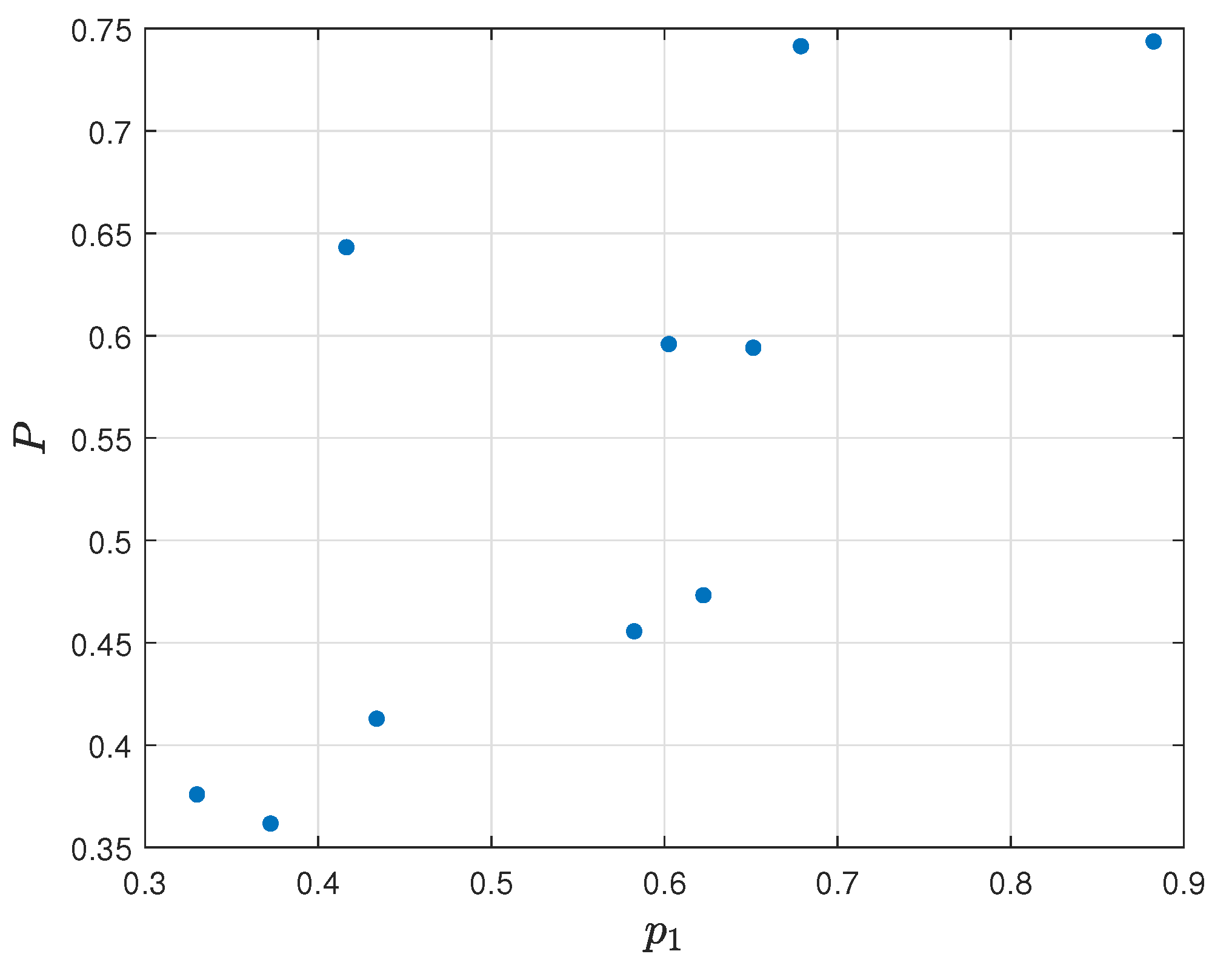
For a better demonstration of the relevance of the obtained parameters to the final assessment model P, a $\rho$ Spearman’s rank correlation coefficient was calculated. $\rho$ Spearman’s rank correlation coefficient between the $P_1$, $P_2$, and $P_3$ model and final ranking P is equal, respectively, to 0.5122, 0.6679, and 0.3182. The correlation between the first two models is moderately strong, and, in the case of the third model, the correlation is weak. 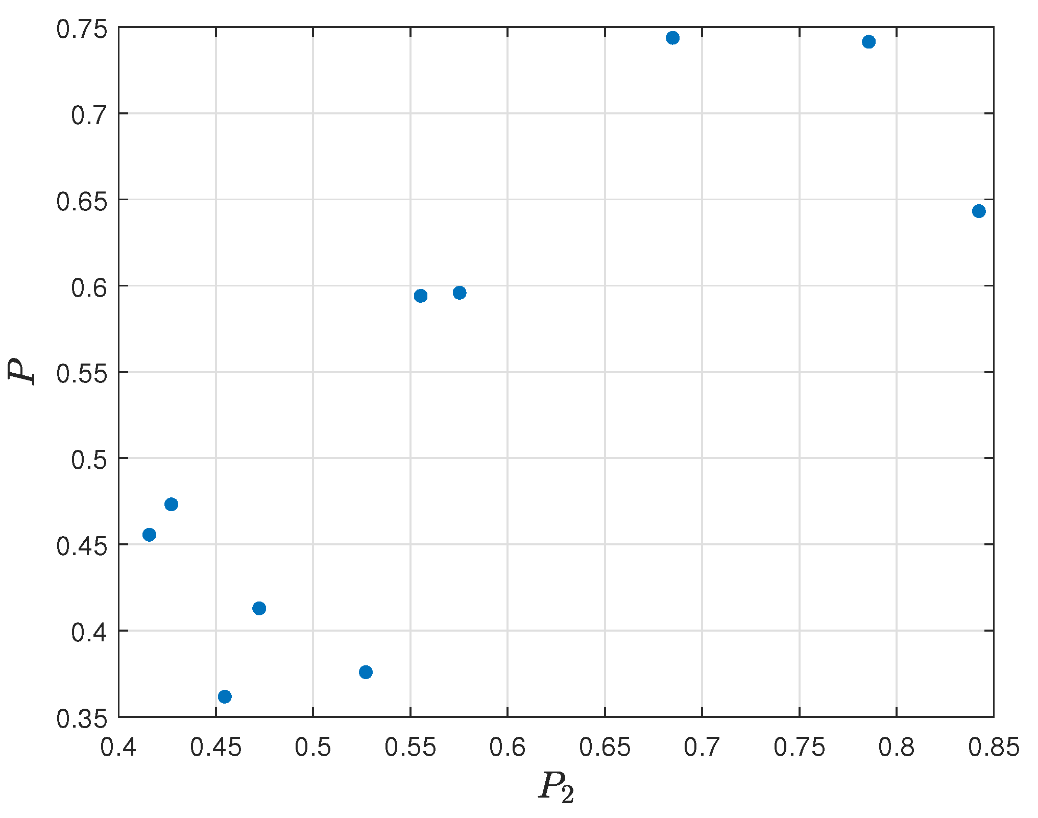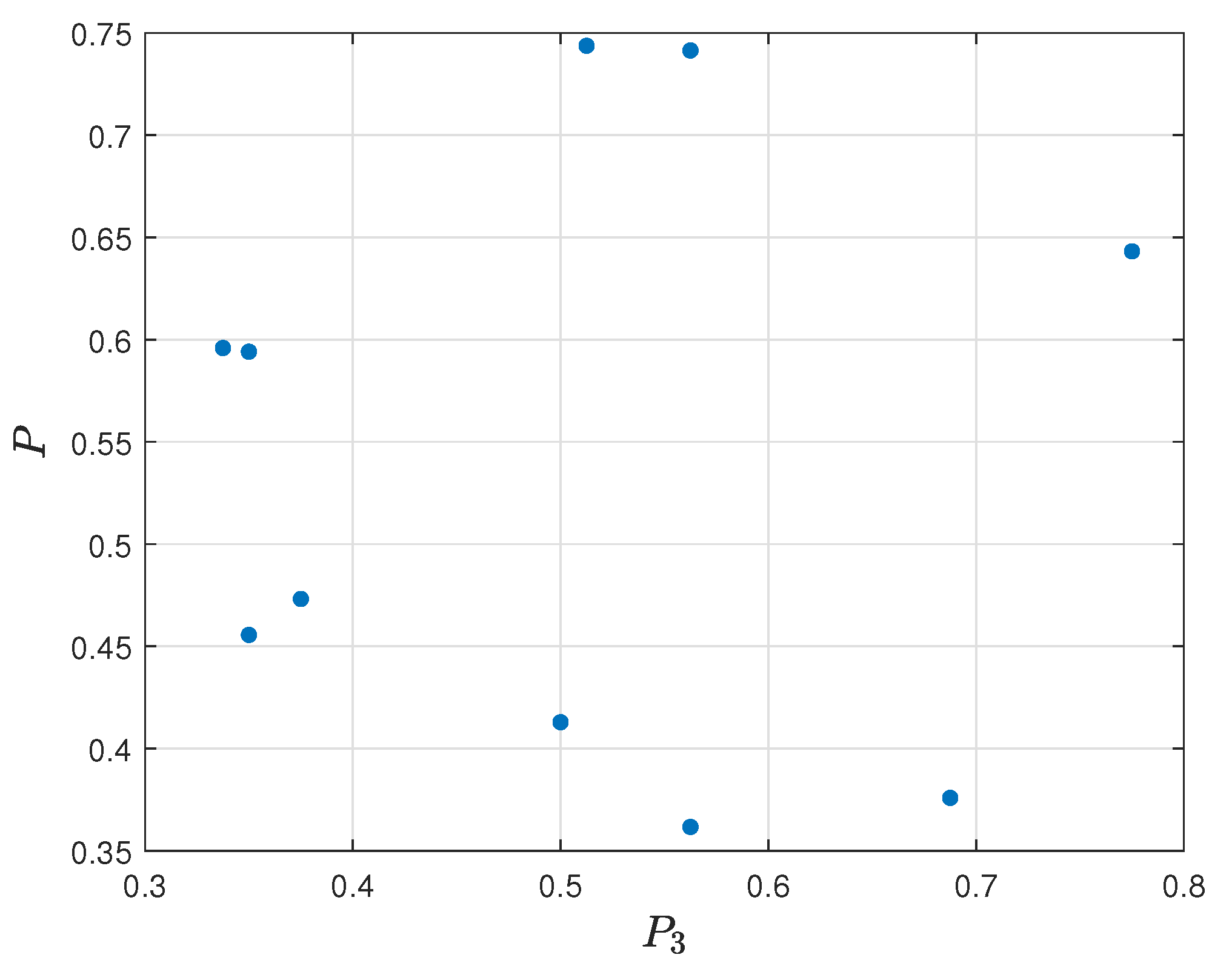The visualization of the relation diagram of effectiveness per round ($P_1$) and final assessment P is shown in Figure 19, the relation diagram of frag gaining ($P_2$) and final assessment P is presented in Figure 20, and the relation diagram of failures per round ($P_3$) and final assessment P is presented in Figure 21.

The sample data for the top 10 players is shown in

Table 10. The performance table of the assessment models $P_1$–$P_3$, final assessment P with their rankings.

Pos.	Name	${\mathit{P}}_1$	${\mathit{P}}_2$	${\mathit{P}}_3$	P	$\mathit{Rank}{\mathit{P}}_1$	$\mathit{Rank}{\mathit{P}}_2$	$\mathit{Rank}{\mathit{P}}_3$	$\mathit{Rank}\mathit{P}$
1	s1mple	0.8825	0.6849	0.5125	0.7437	1	3	3	1
2	ZywOo	0.6788	0.7857	0.5625	0.7414	2	2	10	2
3	Jame	0.4163	0.8423	0.7750	0.6432	4	1	2	3
4	Jamppi	0.6513	0.5553	0.3500	0.5941	7	5	9	5
5	huNter	0.6025	0.5753	0.3375	0.5959	5	4	1	4
6	vsm	0.5825	0.4158	0.3500	0.4556	6	10	8	7
7	meyern	0.6225	0.4271	0.3750	0.4732	8	8	7	6
8	Kaze	0.4338	0.4723	0.5000	0.4129	3	9	4	8
9	Hatz	0.3725	0.4546	0.5625	0.3617	9	7	6	10
10	Sico	0.3300	0.5271	0.6875	0.3759	10	6	5	9

. The final decision assessment model identified ‘Simple’ as the best player at all when the worst rating was given to ’Hatz’. Analyzing the results of the three related models, we can conclude that the highest score in the first model ($P_1$) was obtained by ‘Simple’ again, and is equal to 0.8825. In the ($P_2$) and $P_3$ models, the best outcome was acquired by ‘Jame’ with the value 0.8423 as $P_2$ and 0.7750 as $P_3$. The interesting fact is that ‘ZywOo’, who placed the second position, even if he did not have the best score in any of the three models, was still better than Jame. ‘ZywOo’ received a much better result in the first model and had a comparable score to ‘Jame’ in the second model. Furthermore, ‘huNter’ with the fourth result was close to beat ‘Jame’ and take over his position. In comparison with ‘Jame’, ‘huNter’ had much higher assessment in $P_1$, getting average results at the rest of the models. It follows from this that the most critical models are $P_1$ and $P_2$.

$\rho$ Spearman’s rank correlation coefficient between the $P_1$, $P_2$, and $P_3$ model and reference ranking is equal, respectively, to 0.7818, 0.7091, and 0.0061. The correlation between the first two models is moderately strong, and, in the case of the third model, there is no correlation. However, $\rho$ Spearman’s coefficient between the final model and reference ranking is equal to 0.9636, which means that both rankings are strongly correlated, and the proposed structure of the assessment model well defines the investigated relationships.

6. Practical Exploitation of the Identified Model

This section proposes and applies the own players’ assessment model using a hierarchical structure with the application of COMET method. It describes every related assessment model and shows the final summary and obtained results for the top 40 professional players in CS: GO game. The performance table is presented in

Table 11. The performance table of the alternatives, selected criteria, and reference ranking.

Pos.	Name	${\mathit{C}}_1$	${\mathit{C}}_2$	${\mathit{C}}_3$	${\mathit{C}}_4$	${\mathit{C}}_5$	${\mathit{C}}_6$	$\mathit{Rating}2.0$
1	s1mple	0.88	86.6	1958	1.50	0.09	0.59	1.34
2	ZywOo	0.83	85.3	4151	1.40	0.12	0.59	1.32
3	Jame	0.78	79.3	3505	1.51	0.09	0.52	1.29
4	Jamppi	0.83	83.1	2851	1.30	0.1	0.64	1.25
5	huNter	0.80	88.2	4100	1.22	0.15	0.66	1.24
6	vsm	0.80	86.6	2420	1.22	0.13	0.65	1.24
7	meyern	0.82	83.8	1728	1.28	0.12	0.64	1.24
8	Kaze	0.78	80.7	1750	1.32	0.1	0.60	1.24
9	Hatz	0.76	81.8	2017	1.28	0.15	0.60	1.23
10	Sico	0.76	78.4	1876	1.36	0.13	0.56	1.23
11	yuurih	0.79	87.1	3833	1.24	0.15	0.63	1.22
12	aliStair	0.77	78.7	2028	1.32	0.12	0.58	1.22
13	TenZ	0.80	85.5	2406	1.22	0.13	0.65	1.22
14	xsepower	0.76	75.6	3856	1.31	0.09	0.58	1.21
15	roeJ	0.80	87.7	2338	1.18	0.14	0.68	1.21
16	floppy	0.79	84.3	3251	1.32	0.14	0.65	1.21
17	Brehze	0.80	83.3	2492	1.22	0.12	0.65	1.21
18	KSCERATO	0.75	79.4	3637	1.35	0.12	0.56	1.21
19	electronic	0.76	83.9	1631	1.21	0.14	0.62	1.21
20	EliGE	0.77	84.8	2900	1.19	0.14	0.65	1.20
21	woxic	0.77	80.5	1699	1.25	0.11	0.61	1.20
22	kNgV-	0.78	79.8	1964	1.27	0.09	0.62	1.20
23	INS	0.74	83.8	1961	1.19	0.18	0.62	1.19
24	BnTeT	0.73	81.2	1516	1.23	0.15	0.59	1.19
25	erkaSt	0.79	83.3	2076	1.22	0.14	0.65	1.19
26	somedieyoung	0.78	84.6	2398	1.19	0.14	0.65	1.19
27	NAF	0.72	82.2	2717	1.18	0.16	0.61	1.19
28	NiKo	0.78	83.9	2066	1.18	0.12	0.67	1.18
29	dexter	0.76	82.2	2047	1.18	0.14	0.65	1.18
30	kennyS	0.77	78.6	2934	1.24	0.1	0.62	1.18
31	jks	0.76	82.7	1741	1.19	0.12	0.64	1.18
32	blameF	0.75	83.3	2474	1.18	0.16	0.64	1.18
33	shz	0.80	83.0	2009	1.24	0.13	0.65	1.18
34	nexa	0.75	80.3	3819	1.24	0.13	0.60	1.18
35	Bubzkji	0.76	85.2	3186	1.16	0.13	0.66	1.18
36	Texta	0.76	83.1	2097	1.15	0.16	0.66	1.18
37	coldzera	0.78	82.2	1767	1.22	0.11	0.64	1.18
38	frozen	0.75	81.2	2789	1.19	0.14	0.63	1.17
39	MarKE	0.74	80.9	1851	1.17	0.13	0.63	1.17
40	mantuu	0.77	82.0	2755	1.16	0.12	0.67	1.17

.

The performance table of the selected criteria $C_1$, $C_2$ and assessment model $P_1$ is presented in

Table 12. The performance table of the selected criteria $C_1$, $C_2$ and assessment model $P_1$.

Pos.	Name	${\mathit{C}}_1$	${\mathit{C}}_2$	${\mathit{P}}_1$
1	s1mple	0.88	86.6	0.8825
2	ZywOo	0.83	85.3	0.6788
3	Jame	0.78	79.3	0.4163
4	Jamppi	0.83	83.1	0.6513
5	huNter	0.80	88.2	0.6025
6	vsm	0.80	86.6	0.5825
7	meyern	0.82	83.8	0.6225
8	Kaze	0.78	80.7	0.4338
9	Hatz	0.76	81.8	0.3725
10	Sico	0.76	78.4	0.3300
11	yuurih	0.79	87.1	0.5513
12	aliStair	0.77	78.7	0.3712
13	TenZ	0.80	85.5	0.5688
14	xsepower	0.76	75.6	0.2950
15	roeJ	0.80	87.7	0.5963
16	floppy	0.79	84.3	0.5163
17	Brehze	0.80	83.3	0.5413
18	KSCERATO	0.75	79.4	0.3050
19	electronic	0.76	83.9	0.3988
20	EliGE	0.77	84.8	0.4475
21	woxic	0.77	80.5	0.3937
22	kNgV-	0.78	79.8	0.4225
23	INS	0.74	83.8	0.3225
24	BnTeT	0.73	81.2	0.2525
25	erkaSt	0.79	83.3	0.5038
26	somedieyoung	0.78	84.6	0.4825
27	NAF	0.72	82.2	0.2275
28	NiKo	0.78	83.9	0.4738
29	dexter	0.76	82.2	0.3775
30	kennyS	0.77	78.6	0.3700
31	jks	0.76	82.7	0.3838
32	blameF	0.75	83.3	0.3538
33	shz	0.80	83.0	0.5375
34	nexa	0.75	80.3	0.3163
35	Bubzkji	0.76	85.2	0.415
36	Texta	0.76	83.1	0.3887
37	coldzera	0.78	82.2	0.4525
38	frozen	0.75	81.2	0.3275
39	MarKE	0.74	80.9	0.2863
40	mantuu	0.77	82.0	0.4125

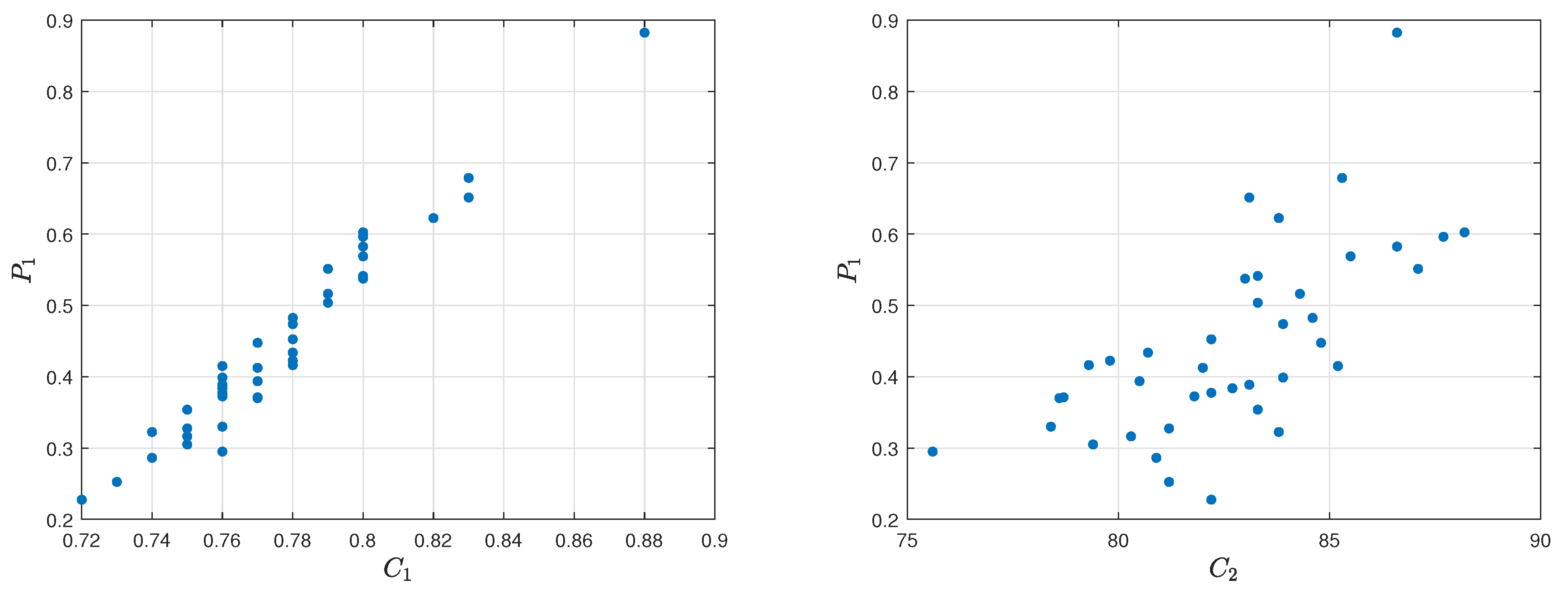
. For a better demonstration of the relevance of the criteria to the $P_1$ assessment model, a $\rho$ Spearman’s rank correlation coefficient was calculated. $\rho$ Spearman’s rank correlation coefficient between the criteria $C_1$, $C_2$ and reference ranking obtained by $P_1$ assessment model is equal to 0.6670 and 0.2420. The correlation between the first one is moderately strong, while, in the second one, it is weak. The visualization of the relation diagram of Average kills per round ($C_1$) and $P_1$ assessment model, as well as the relation diagram of Average damage per round ($C_2$) and $P_1$ assessment model, is presented in Figure 22. The $P_2$ and $P_3$ models were analyzed, as well, and their results presented in an analogical way. The whole process can be found in Appendix A.

The sample data for the top 40 players is shown in

Table 13. The performance table of the related assessment models and final ranking.

Pos.	Name	${\mathit{P}}_1$	${\mathit{P}}_2$	${\mathit{P}}_3$	P	$\mathit{Ranking} \mathit{P}$
1	s1mple	0.8825	0.6849	0.5125	0.7437	1
2	ZywOo	0.6788	0.7857	0.5625	0.7414	2
3	Jame	0.4163	0.8423	0.7750	0.6432	3
4	Jamppi	0.6513	0.5553	0.3500	0.5941	5
5	huNter	0.6025	0.5753	0.3375	0.5959	4
6	vsm	0.5825	0.4158	0.3500	0.4556	16
7	meyern	0.6225	0.4271	0.3750	0.4732	11
8	Kaze	0.4338	0.4723	0.5000	0.4129	14
9	Hatz	0.3725	0.4546	0.5625	0.3617	18
10	Sico	0.3300	0.5271	0.6875	0.3759	7
11	yuurih	0.5513	0.5798	0.4500	0.5545	6
12	aliStair	0.3712	0.4985	0.6000	0.3882	13
13	TenZ	0.5688	0.4145	0.3500	0.4496	17
14	xsepower	0.2950	0.6613	0.5500	0.5057	34
15	roeJ	0.5963	0.3480	0.2500	0.4290	33
16	floppy	0.5163	0.6145	0.3625	0.5912	15
17	Brehze	0.5413	0.4225	0.3375	0.4494	30
18	KSCERATO	0.3050	0.6834	0.6750	0.4975	8
19	electronic	0.3988	0.3260	0.4750	0.2869	22
20	EliGE	0.4475	0.4162	0.3625	0.4048	20
21	woxic	0.3937	0.3923	0.4750	0.3392	25
22	kNgV-	0.4225	0.4389	0.4000	0.4055	35
23	INS	0.3225	0.3273	0.5250	0.2488	12
24	BnTeT	0.2525	0.0000	0.6000	0.1021	26
25	erkaSt	0.5038	0.3833	0.3625	0.3980	10
26	somedieyoung	0.4825	0.3688	0.3625	0.3786	40
27	NAF	0.2275	0.3840	0.5375	0.2583	9
28	NiKo	0.4738	0.3223	0.2625	0.3613	28
29	dexter	0.3775	0.3205	0.3625	0.3016	37
30	kennyS	0.3700	0.4945	0.4250	0.4261	21
31	jks	0.3838	0.3063	0.3750	0.2893	38
32	blameF	0.3538	0.3610	0.4250	0.3114	32
33	shz	0.5375	0.4067	0.3500	0.4322	29
34	nexa	0.3163	0.5785	0.5375	0.4487	31
35	Bubzkji	0.4150	0.3985	0.3125	0.3906	19
36	Texta	0.3887	0.2800	0.3500	0.2756	36
37	coldzera	0.4525	0.3538	0.3625	0.3556	27
38	frozen	0.3275	0.4058	0.4375	0.3355	23
39	MarKE	0.2863	0.2868	0.4250	0.2266	39
40	mantuu	0.4125	0.3575	0.2625	0.3682	24

. The final decision assessment model identified ‘Simple’ as the best player at all with an excellent value equal to 0.7437, when the worst rating was given to ‘BnTeT’, who received value equal to 0.1021. Analyzing the results of the three related models, we can conclude that the highest score in the first model $P_1$ was obtained by ‘Simple’ again, and is equal to 0.8825, while the lowest score received by ’NAF’ was only 0.2275. In the $P_2$ and $P_3$ models, the best outcome was acquired by ‘Jame’ with the value 0.8423 as $P_2$ and 0.7750 as $P_3$. The worst assessment in $P_2$ was given to ‘BnTeT’ with the value 0, and in the $P_3$ model the lowest evaluation value was given to ‘roeJ’ with the value 0.2500. The interesting fact is that ‘ZywOo’, who placed the second position, even if he did not have the best score in any of the three models, was still better than Jame. ‘ZywOo’ received a much better result in the first model and had a comparable score to ‘Jame’ in the second model. Furthermore, ‘huNter’ with the fourth result was close to beat ‘Jame’ and take over his position. In comparison with ‘Jame’, ‘huNter’ had much higher assessment in $P_1$, getting average results at the rest of the models. It follows from this that the most critical models are $P_1$ and $P_2$.

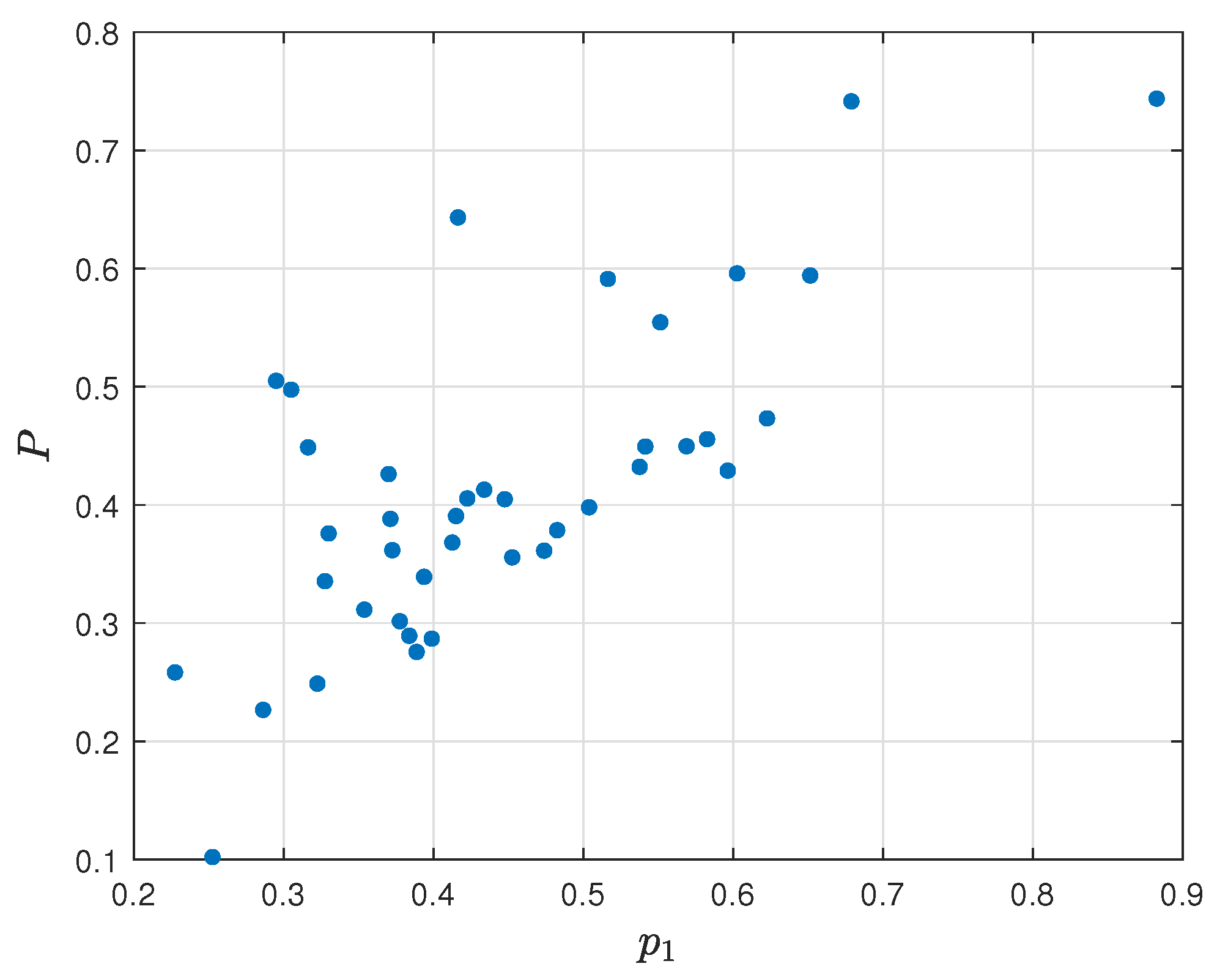
To show the relation of the obtained parameters with the final assessment model P, a $\rho$ Spearman’s rank correlation coefficient was calculated. $\rho$ Spearman’s rank correlation coefficient between the $P_1$, $P_2$, and $P_3$ model and final ranking P is equal, respectively, to 0.5122, 0.6679, and 0.3182. The correlation between the first two models is moderately strong, and, in the case of the third model, the correlation is weak. 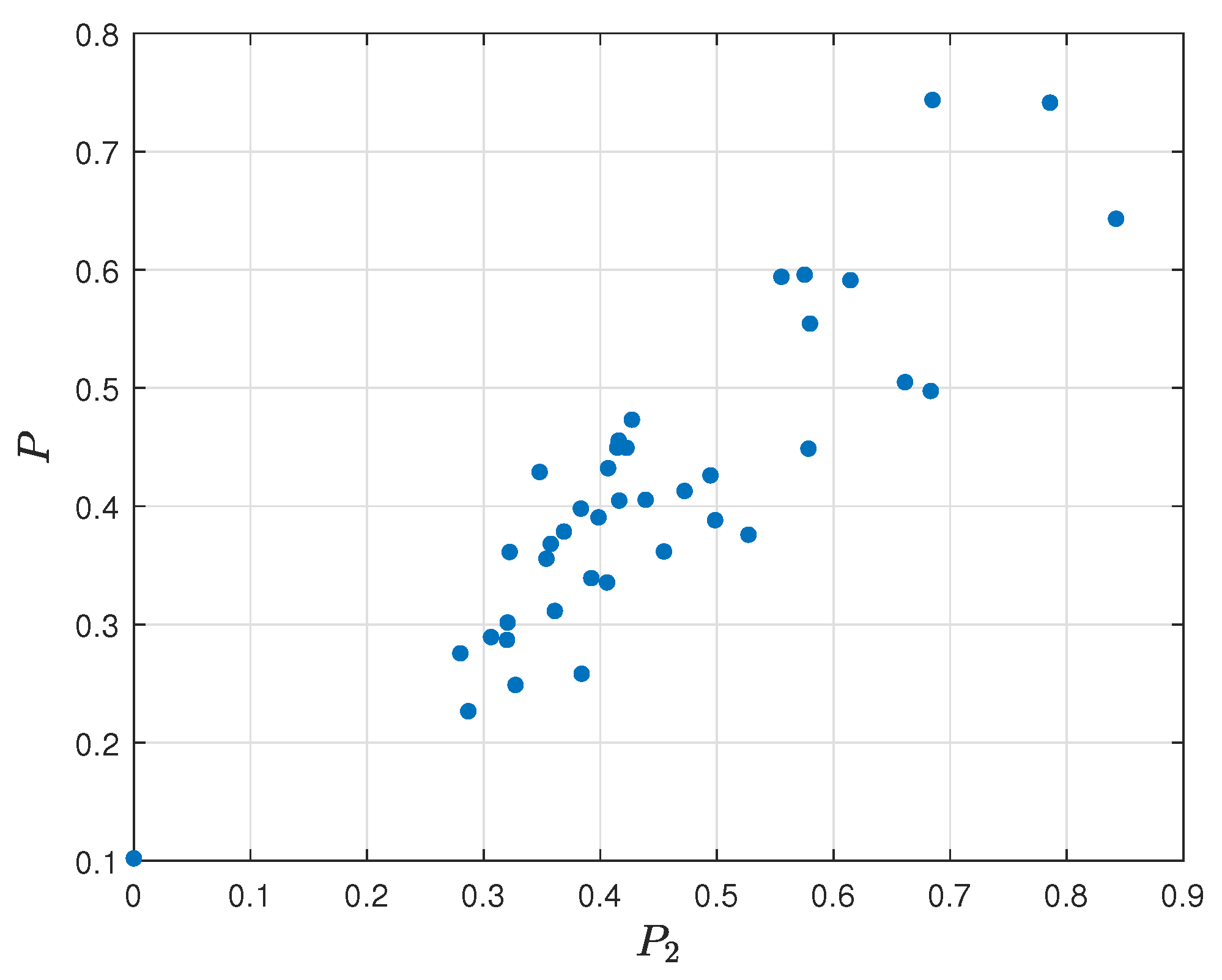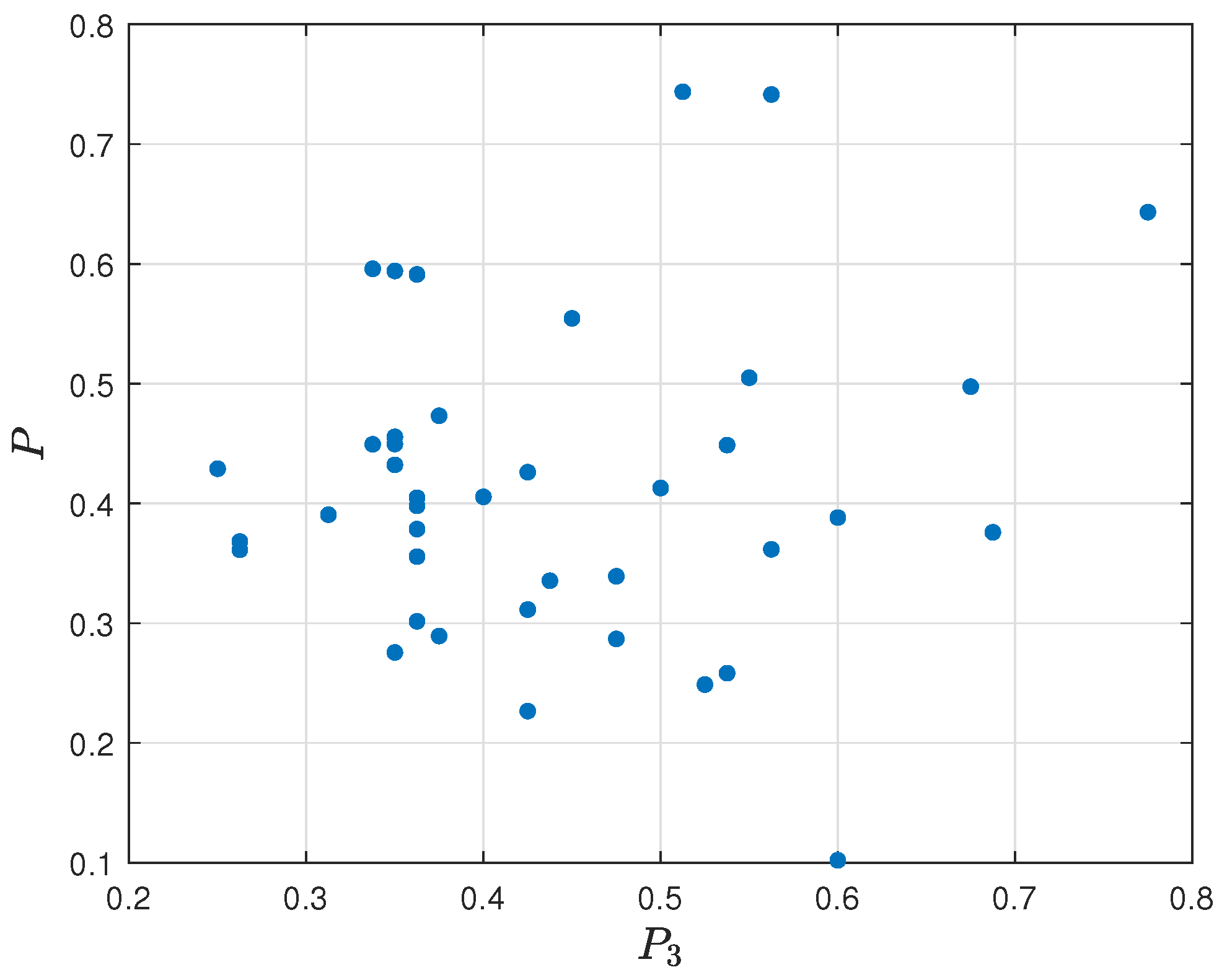The visualization of the relation diagram of effectiveness per round ($P_1$) and final assessment P is shown in Figure 23, the relation diagram of frag gaining ($P_2$) and final assessment P is presented in Figure 24, and the relation diagram of failures per round ($P_3$) and final assessment P is presented in Figure 25.

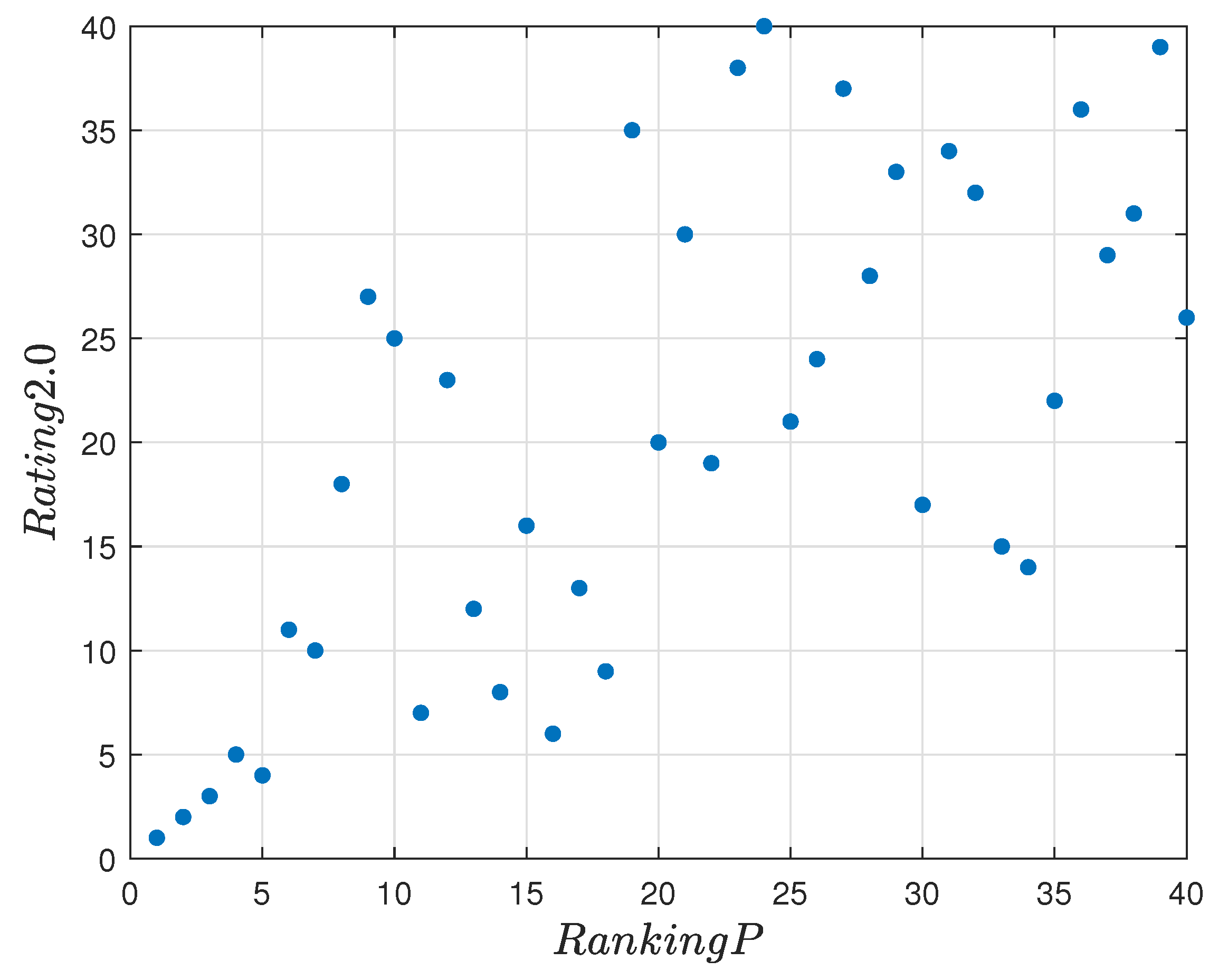
$\rho$ Spearman’s coefficient between the final model and reference ranking is equal to 0.5304, which means that both rankings are moderately correlated. The visualization of the relation diagram of final ranking P and Rating 2.0 is presented in Figure 26.

7. Conclusions

The objective of this work was an identification of the model to create a ranking of players in the popular e-sport game, i.e., Counter-Strike: Global Offensive (CS: GO), using the appropriate multi-criteria decision-making method. For verification purposes, the obtained ranking of players was compared to the existing ranking created by HLTV called Rating 2.0, which is the most prestigious for this game. It was decided to set a ranking for top 10 and, later, even for 40 players. The additional purpose of this paper is to familiarize people with the term of e-sport and to convince them that it is worthwhile and future-proof.

The main contribution of this work is a proposal of the CS: GO players assessment model with three related evaluation models. It was obligatory to choose the right method, build associated models for the players, and then to calculate the player’s assessments for their performances. Comet’s resistant to the rank reversal paradox is a significant feature. That’s not relevant which set of players will be applied, because each of them will always get the same value. The comparison of characteristic objects is easier than the players because the distance between them is bigger than the compared players. The identification of the CS: GO players assessment model additionally allows evaluating every set of players in the considered numerical space without involving the expert in the evaluation process again because the model is defined for a certain set of player characteristics. Another original feature of the COMET method is the employment of global criterion weights, which determine the average significance of a criterion for the final assessment. The linear weighting of non-linear problems reduces the accuracy of the results. That is the reason why the calculation procedure of this method has resigned from arbitrary weights for specific criteria. Therefore, the COMET method was chosen as the best approach to make an identification of the players’ assessment model.

The results demonstrate that the model could be utilized to evaluate the players and helps to generate the ranking and select the best CS: GO player. The positions of incorrectly classified players are quite close to each other. $\rho$ Spearman’s coefficient between the final model and reference ranking is equal to 0.5304, which means that both rankings are moderately correlated. Despite quite an average result, this ranking might be considered as sufficient, because the top positions of the classification are more fitted to reference ranking. The proposed structure of the assessment model satisfactorily defines the investigated relationships.

Further future work directions should concentrate on the improvement of model effectiveness. Perhaps adding a greater amount of input criteria, and thus increasing the number of related assessment models, could make the final ranking more reliable and appropriate to reflect some players real talent. Moreover, this should fix on the prospective empirical investigation for CS: GO game but also in other e-sport games.