Design and Implementation of a Graphic Simulator for Calculating the Inverse Kinematics of a Redundant Planar Manipulator Robot

Abstract

In this paper, a graphics simulator that allows for characterizing the kinematic and dynamic behavior of redundant planar manipulator robots is presented. This graphics simulator is implemented using the Solidworks software and the SimMechanics Toolbox of MATLAB/Simulink. To calculate the inverse kinematics of this type of robot, an algorithm based on the probabilistic method called Simulated Annealing is proposed. By means of this method, it is possible to obtain, among many possibilities, the best solution for inverse kinematics. Without losing generality, the performance of metaheuristic algorithm is tested in a 6-DoF (Degrees of Freedom) virtual robot. The Cartesian coordinates (x,y) of the end effector of the robot under study can be accessed through a graphic interface, thereby automatically calculating its inverse kinematics, and yielding the solution set with the position adopted by each joint for each coordinate entered. Dynamic equations are obtained from the Lagrange–Euler formulation. To generate the joint trajectories, an interpolation method with a third order polynomial is used. The effectiveness of the developed methodologies is verified through computational simulations of a virtual robot.

1. Introduction

Nowadays, the use of manipulator robots is widely extended in the industry because these robots carry out tasks that pose risks to humans, improve the quality of the products manufactured, and increase productivity. Nevertheless, robotics is not limited to the industry, but has also expanded to other fields such as medicine (robotic implants or remote surgical intervention systems), agriculture (sheep shearing or pork cutting), space (planetary surface exploration), and geological and military research, among others [1,2,3].

Manipulator robots can be classified into serial and parallel based on their structure. The links of a serial manipulator are normally assembled together by means of rotational or prismatic joints that form an open kinematic chain whose structure is similar to a human arm. This configuration allows for assembling a clamp or any other tools that can be moved to any position within the robot’s workspace [4].

The industrial robots available in the global markets are not redundant, but they do have the degrees of freedom necessary for performing the tasks for which they were designed [5]. However, if a failure occurs in the actuator of an industrial robot, without a safety backup, its respective joint blocks, and the robot losses the mobility of that joint. This may lead to situations that imply risks to the operators, difficulties for the users, interruption of the mining or industrial process, and economic losses, among other consequences [6]. Therefore, interest has arisen in the study of the behavior of redundant manipulator robots, owing to a design that gives them more degrees of freedom than necessary for performing a specific task [7].

In general, the kinematic and dynamic study of robotic systems can be conducted in a didactic way, using graphic simulators. The kinematic problem can be solved through the Geometric Method, but, in practice, this method is not widely used because of the complexity of applying it to redundant manipulator robots, which has led to the development of several alternative methods. Kinematics is divided into direct and inverse kinematics (IK) that can be derived based on the standard Denavit-Hartenberg (D-H) model, which describes the geometry of the robot. Besides the almost universally used the D-H parameters [8,9,10,11], other methods such Algebra and Lie Groups are also useful to obtain the kinematics of the system [12].

The inverse kinematics chain of redundant manipulator robots is much more difficult to obtain. Its solution is fundamental to deal with problems such as route planning, visually guided movement, grabbing objects, etc. [13]. Currently, the conventional methods for solving inverse kinematics are divided into two categories: analytical (geometric-algebraic) and numerical (iterative algorithms) [14]. Some recent articles show that analytical solutions have only been found for some specific structures of redundant manipulator robots. For instance, Qian et al. [15] present a close loop intuitive solution for a space manipulator robot with 7-DoF and a PYR-P-PYR (Pitch-Yaw-Roll) structured based on the blockage of the first joint P. Teja and Shah [16] present the Inverse Coordinates Method for a special S-RRR (Spherical-Rotary) configuration, which is based on the inversion of the base and the end effector of the manipulator robot. Additionally, Zhao et al. [17] employ analytical, geometric and algebraic methods for a 6R industrial robot, which are combined with the Paden–Kahan subproblem and the matrix theory.

Furthermore, since there are no possible analytical solutions for the inverse kinematics of some robots, some methods are now under discussion, for example, the Iterative Method, which is based on numerical methods [18]. Huang and Nie [19] present a numerical solution, which is achieved through the application of the Sequential Recovery Method to a robot with and RPY (Roll-Pitch-Yaw) configuration based on the modification of the Newton-Raphson Method. Another alternative to obtain the inverse kinematics is using the $J^T$ transpose or the $J^{-1}$ inverse of the Jacobian matrix [20]. The usefulness of the $J^T$ Jacobian is demonstrated by Besset and Taylor [21]. In addition, Farzan and DeSouza [22] show a solution based on estimates of the inverse Jacobian matrix.

Recently, as some traditional methods have become obsolete for some manipulator robots, researchers have started the development or artificial intelligence techniques for calculating inverse kinematics. Among these techniques or meta-heuristic algorithms, artificial neural networks (ANNs), genetic algorithms (GAs), particle swarm optimization (PSO), artificial bee colony (ABC), differential evolution (DE) and simulated annealing (SA) stand out. Köker and Cakar [23] propose a hybrid smart solution for IK, which includes ANN, GA and SA and is applied to a 4-DoF robot. The weak point of this study is that optimization processes based on SA have a prolonged execution time due to the difficulties to select suitable cooling parameters. López et al. [24] present different meta-heuristic algorithms to solve the inverse kinematics of a KUKA Youbot mobile robot with 9-DoF. From simulations and real experimental results, it is demonstrated the superiority of the DE algorithm over other algorithms due to its computational cost, reduced joint movement and minimum error between the end effector and the target point. Additionally, López et al. [24] demonstrate that the hybrid biogeography-based optimization (HBBO) approach generates good results but with high computational costs. In contrast, cuckoo search (CS) and PSO report poor results and are not suggested as methods for obtaining inverse kinematics. The flaw of this study regarding the DE algorithm, is the number of iterations used, which slows down the search for a solution. Dereli and Köker [25] compare the position error and calculation time of two heuristic techniques called PSO and ABC. The simulations show that both algorithms successfully find the angles of the joints of a redundant manipulator robot with 7-DoF. Despite its good performance, the long steps of the search process and the excess of parameters are considered the disadvantages of this method. The algorithms above suffer a common problem: the time consumed during the iteration process. In this regard, Zhou et al. [26] propose a smart algorithm based on extreme machine learning (ELM) and sequential mutation genetic algorithm (SGA) to improve the efficiency of the Standford MT-ARM manipulator robot of 6-DoF. Nevertheless, this last study sacrificed the accuracy of the preliminary solution of inverse kinematics.

Currently, several researchers have implemented simulation systems them in robots [24,26,27] because they allow for manipulating and testing the control system of automated robot within a virtual environment. For example, Kereluk and Emani [28] present an integrated design and simulation environment that offers control over the hardware of a reconfigurable manipulator robot with 18-DoF denominated MARS. In this environment, the user can select or design the configuration of the manipulator robot, simulate its operation in a virtual reality environment and operate the physical manipulator robot. The simulation results have proved to be very similar to experimental results. López et al. [24] developed a simulator on MATLAB software to test the performance of different meta-heuristic algorithms for solving the inverse kinematics of manipulator robots. Zhou et al. [26] also used it to analyze, specifically, time efficiency during the training stage of NNs and ELM, as well as for the optimization and computational process.

The contribution of this study is the development (design and implementation) of a graphic simulator using the Solidworks software and the SimMechanics Toolbox from MATLAB/Simulink. This program is commanded from a graphic interface that is created with the MATLAB tool GUIDE. GUIDE allows for characterizing kinematic and dynamic behavior; additionally, tests can be conducted in the control system of a planar manipulator robot with 6-DoF within a virtual environment. An innovative aspect of this work is that the special configuration of the 6-DoF manipulator robot, which includes rotational and prismatic (linear) joints. Most recent research employs robot structures with rotational joints and omit linear ones. Exploring new types of configurations allow for improving the skills of the robot, broadening its workspace, increasing its accuracy, or improving its energy consumption [28]. The SA algorithm will be applied to the manipulator robot without adding any other meta-heuristic algorithm. Additionally, before using SA, an algorithm to help search for the initial solution (end effector initial position) will be implemented to enable the end effector to be as close as possible to the set point and will contribute to a faster convergence of the initial solution.

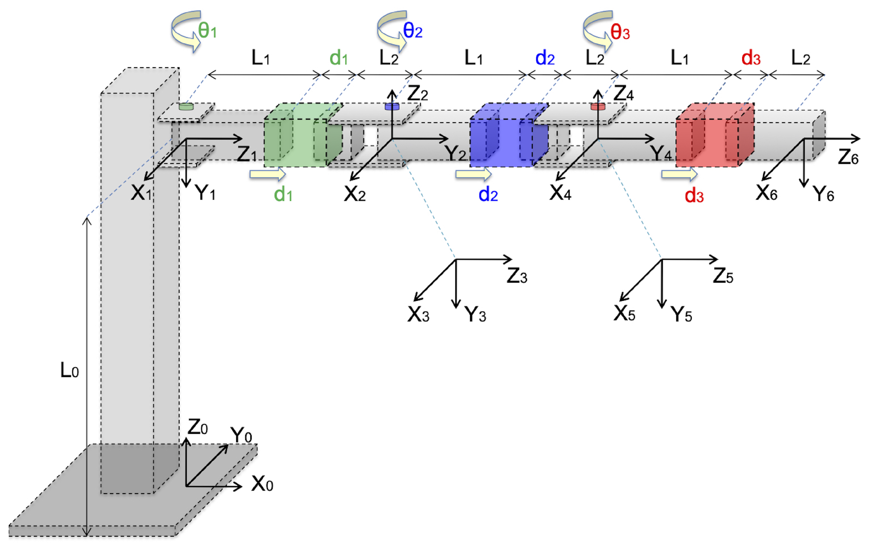
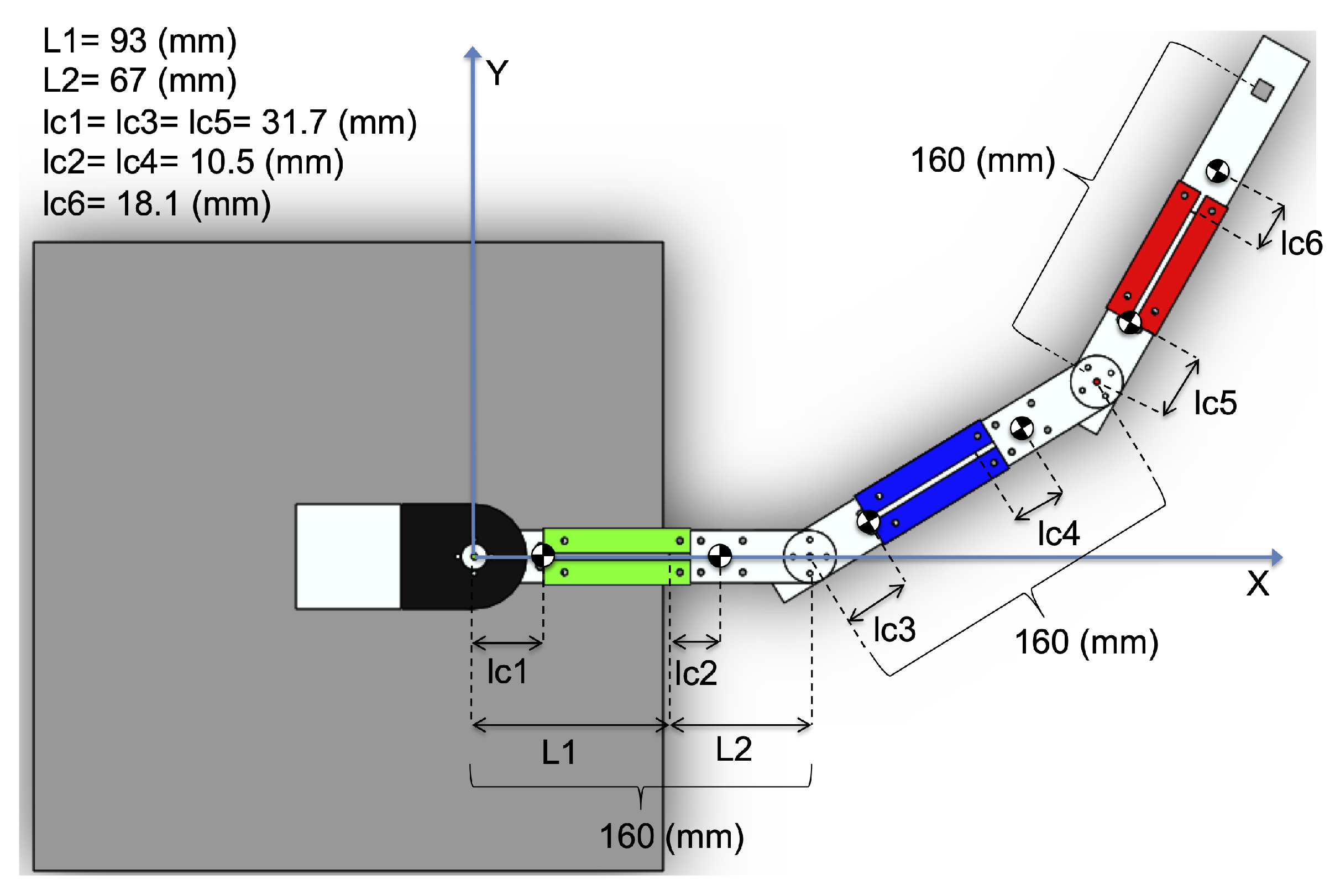
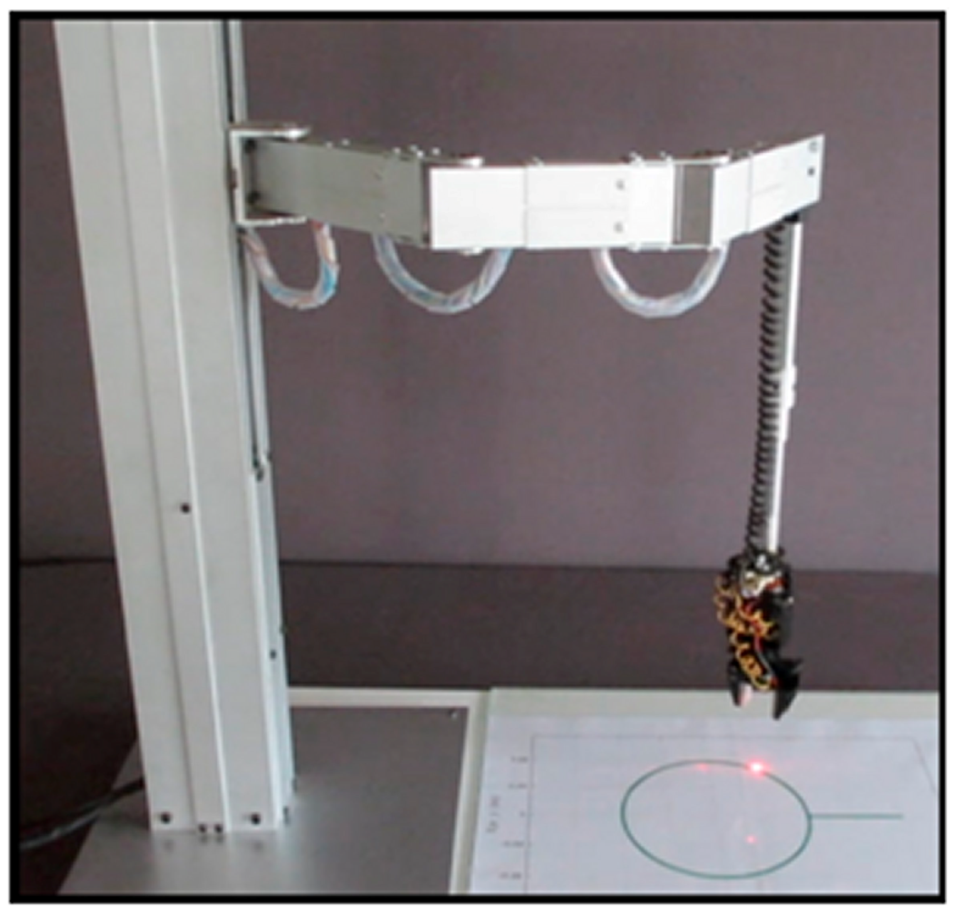
2. Description of the 6-Dof Redundant Planar Manipulator Robot

This work considers a novel 6-DoF redundant planar manipulator robot with three rotary (R) and three prismatic (P) joints arranged in a RPRPRP configuration. If we draw an analogy with a human arm, this robot is composed of three parts: an arm, a first forearm and a second forearm. Each part is made up of two links and two types of joints (rotary and prismatic).

This redundant planar manipulator robot constitutes an open kinematic chain that originates from the assembling of the rotary joint, specifically between its fixed base and the arm; the arm and the first forearm, and, finally, the first and second forearm. Additionally, the prismatic joints connect the links as follows: first and secondary link, third and fourth link, and fifth and sixth link.

3. Kinematic Analysis

This section is concerned with the development of the mathematical relationships that analytically describe the spatial motion of the redundant planar manipulator robot under study, without considering the causes of the same. The equations relate the position and orientation of the end part of the robot with the coordinates of the robot joints. This is carried out using a reference system arbitrarily chosen, but that is usually placed on the base of the redundant planar manipulator robot.

Forward Kinematics of the 6-Dof Redundant Planar Manipulator Robot

The D-H method is used to characterize the kinematic behavior of the redundant planar manipulator robot. Taking the axes assigned in the geometrical configuration shown in Figure 1, it is possible to obtain the robot joint parameters, which are presented in

Table 1. Joint parameters of the 6-DoF redundant planar manipulator robot.

Joint	${\mathit{\theta }}_{\mathit{i}}$	${\mathit{d}}_{\mathit{i}}$	${\mathit{a}}_{\mathit{i}}$	${\mathit{\alpha }}_{\mathit{i}}$
1	${\theta }_1^{*}-{90}^{\circ }$	$L_0$	0	$-{90}^{\circ }$
2	$0^{\circ }$	$d_1^{*}+L_1+L_2$	0	${90}^{\circ }$
3	${\theta }_2^{*}$	0	0	$-{90}^{\circ }$
4	$0^{\circ }$	$d_2^{*}+L_1+L_2$	0	${90}^{\circ }$
5	${\theta }_3^{*}$	0	0	$-{90}^{\circ }$
6	$0^{\circ }$	$d_3^{*}+L_1+L_2$	0	$0^{\circ }$

.

The homogeneous transformation matrix of Equation (1) is completely defined based on joint parameters:

$${\mathbf{A}}_i^{i-1}\left(q_i\right)=\left[\begin{array}{cccc}cos\left({\theta }_i\right)& -sin\left({\theta }_i\right)cos\left({\alpha }_i\right)& sin\left({\theta }_i\right)sin\left({\alpha }_i\right)& a_{i}cos\left({\theta }_i\right)\\ sin\left({\theta }_i\right)& cos\left({\theta }_i\right)cos\left({\alpha }_i\right)& -cos\left({\theta }_i\right)sin\left({\alpha }_i\right)& a_{i}sin\left({\theta }_i\right)\\ 0& sin\left({\alpha }_i\right)& cos\left({\alpha }_i\right)& d_i\\ 0& 0& 0& 1\end{array}\right]$$

(1)

where: $i=1,\dots .,6$.

According to the D-H convention, the product of each transformation matrix that link the coordinate system $0_{i-1}$ is calculated with the immediately after $0_i$, and the 4x4 $\mathbf{T}$ matrix is obtained, which represents the pose (position and orientation) of the last link from the base system.

$$\mathbf{T}={}^0{\mathbf{A}}_1{}^1{\mathbf{A}}_2{}^2{\mathbf{A}}_3{}^3{\mathbf{A}}_4{}^4{\mathbf{A}}_5{}^5{\mathbf{A}}_6$$

(2)

Then, from $\mathbf{T}$ the following analytical representation of the position of the last link in the base system (coordinates origin) is obtained:

$$x=r_{1}cos\left({\theta }_1\right)+r_{2}cos({\theta }_1+{\theta }_2)+r_{3}cos({\theta }_1+{\theta }_2+{\theta }_3)$$

(3)

$$y=r_{1}sin\left({\theta }_1\right)+r_{2}sin({\theta }_1+{\theta }_2)+r_{3}sin({\theta }_1+{\theta }_2+{\theta }_3)$$

(4)

where: $r_1=d_1+L_1+L_2;r_2=d_2+L_1+L_2;r_3=d_3+L_1+L_2$

4. Direct Dynamics of the 6-Dof Redundant Planar Manipulator Robot

To obtain the dynamic equations of the 6-DoF redundant planar manipulator robot, the L-E Method is applied to the robot shown in Figure 2. Taking into account the prismatic and rotational motions, the generalized coordinate vector is $\mathbf{q}=\left[{\theta }_1{d}_1{\theta }_2{d}_2{\theta }_3{d}_3\right]$.

Where: $l_{ci}$ is the length of the mass center of the link $i,i=1,2,3,4,5,6$.

The dynamic model of the manipulator of 6-DoF, composed of fixed links interconnected by means of joints, can be described in its compact form (matrix), as shown in Equation (5) [29]:

$$\mathbf{\tau }-{\mathbf{\tau }}_0=\mathbf{M}\left(q\right)\ddot{\mathbf{q}}+\mathbf{C}(q,\dot{q})\dot{\mathbf{q}}+\mathbf{G}\left(q\right)+\mathbf{F}\left(q\right)$$

(5)

where: $\mathbf{\tau }$ is the (6 × 1) vector of the generalized forces applied by the actuators on the joints; ${\mathbf{\tau }}_0$ is the (6x1) vector of the input unknown disturbances; $\mathbf{M}$ is the (6×6) inertia matrix; $\mathbf{C}$ is the (6 × 6) centrifugal and Coriolis forces matrix; $\mathbf{G}$ is the (6 × 1) gravitational forces vector; $\mathbf{F}$ is the (6 × 1) vector of the frictions, and $\mathbf{q},\dot{\mathbf{q}},\ddot{\mathbf{q}}$ are the vectors of the joint displacement/angle, speed and acceleration joint vectors, respectively.

Since the manipulator works in a horizontal plane, then $\mathbf{G}\left(q\right)$ is zero (gravity acts perpendicular to the motion plane). Vectors ${\mathbf{\tau }}_0$ and $\mathbf{F}$ are not considered in the construction of the model. The elements of the matrix $\mathbf{M}\left(q\right)$ are presented in Appendix A.

The centrifugal and Coriolis forces matrix $\mathbf{C}(q,\dot{q})$ can be obtained through the Christoffel coefficients $C_{ijk}\left(q\right)$ defined in Equation (6) [30]:

$$C_{ijk}\left(q\right)=\frac{1}{2}\left[\frac{\partial M_{kj}\left(q\right)}{\partial q_i}+\frac{\partial M_{ki}\left(q\right)}{\partial q_j}-\frac{\partial M_{ij}\left(q\right)}{\partial q_k}\right]$$

(6)

where: $M_{ij}\left(q\right)$ denotes the $ij$-th element of the inertia matrix $\mathbf{M}\left(q\right)$. Thus, the $kj$-th element of the $\mathbf{C}(q,\dot{q})$ matrix can be obtained as:

$${\mathbf{c}}_{kj}(q,\dot{q})={\left[\begin{array}{c}{C}_{1jk}\left(q\right)\\ C_{2jk}\left(q\right)\\ ⋮\\ C_{njk}\left(q\right)\end{array}\right]}^T\dot{\mathbf{q}}$$

(7)

Then, the resulting centrifugal and Coriolis forces vector is: $\mathbf{c}(q,\dot{q})=\mathbf{C}(q,\dot{q})\dot{\mathbf{q}}$

Using Equations (6) and (7), the centrifugal and Coriolis forces vector $\mathbf{c}(q,\dot{q})$ shown in Equation (8) is obtained. The components of this vector are presented in Appendix A.

$$\mathbf{c}(q,\dot{q})=\left[C_{i1}\right];i=1,\dots ,6$$

(8)

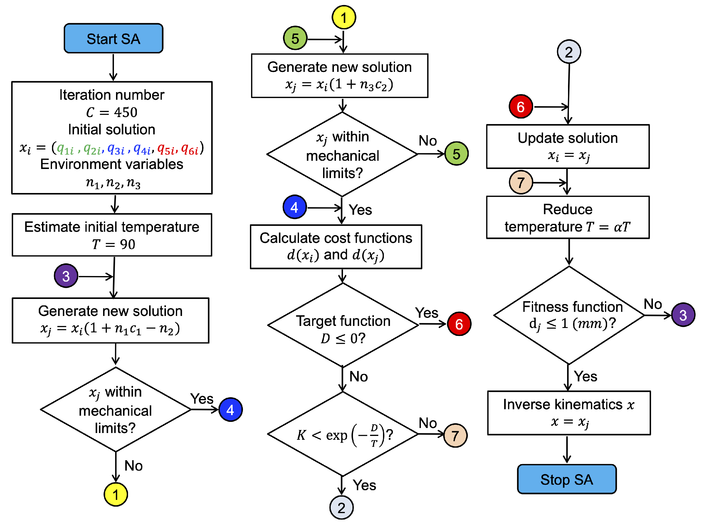
5. Simulated Annealing Algorithm

These days, several methods exist to solve the inverse kinematics of the manipulator robots, but, unfortunately, some of them have long calculation times and only provide one restricted solution [15,31]. In this section, a new method is presented for calculating the inverse kinematics of (standard and redundant) manipulator robots of any type and configuration, based on the probabilistic technique denominated Simulated Annealing (SA).

5.1. Description of the Annealing Process

The physical process called annealing is a technique that consists in heating and then slowly cooling a material to alter its physical and chemical properties. The heat allows atoms to increase their energy, thus making them capable of moving from their initial positions (from a local minimum value of energy to a global one). This occurs because a slow cooling gives atoms higher probabilities of recrystallizing into configurations with lower energy than the initial one. Based on this idea, the SA algorithm was created, which allows conducting a meta-heuristic search for global optimization problems [23].

5.2. Application of the SA Algorithm to the 6-DoF Redundant Planar Manipulator Robot

The SA basic algorithm starts with an iteration number C, an initial state vector $x_i$ of six components (initial solution), that represents the initial inverse kinematics of the robot, and maintains a calculation of a parameter T, commonly called temperature, which is initially high and then is progressively reduced to a value $T_f$ close to zero during the algorithm execution [23]. The configuration of the state and temperature is typically a solution for the function to be optimized. This paper considers an initial temperature $T=$90, C = 450 iterations, and the cooling factor $\alpha =$0.94.

The solution is perturbed in each iteration of the algorithm to produce a new neighbor solution $x_j$ from its neighborhood [32]. The first heuristic perturbation of the initial state $x_i$ occurs according to Equation (9).

$$x_j=x_i(1+n_1{c}_1-n_2)$$

(9)

where: $n_1$ and $n_2$ are the environment variables and $c_1$ is a random number evenly distributed over the (0,1) interval.

Subsequently, it is verified that the value of each component of the $x_j$ vector calculated in Equation (9), which represents the joint position (current inverse kinematics), is within the mechanical limits of the redundant planar manipulator robot. Otherwise, a new calculation of the values for $x_j$ is made using Equation (10).

$$x_j=x_i(1+n_3{c}_2)$$

(10)

where: $n_3$ is an environment variable and $c_2$ is a random scale evenly distributed. This second disturbance of $x_i$, governed by Equation (10) does not stop until each value of the joint variables of $x_j$ is within the allowed limits.

In addition, the quality of both solutions is assessed using a D target function, which is shown in Equation (11). Then, a new state $x_j$ could be eventually selected from the two solutions, as long as $x_j$ is better quality than $x_i$.

$$D=d\left(x_j\right)-d\left(x_i\right)$$

(11)

where: $d\left(x_i\right)$ is the performance of the initial state, and $d\left(x_j\right)$ the performance of the current state, as shown in Figure 3. The calculation of each performance corresponds to the root mean square function shown in Equation (12):

$$d\left(x_k\right)=\frac{\Vert p\left(x\right)-p\left(x_k\right)\Vert }{2}=\frac{d_k}{2};k=i,j$$

(12)

$$x_k=[q_{1k},q_{2k},\dots ,q_{nk}];k=i,j$$

(13)

where: $d_k$ is a cost function, $p\left(x_i\right)$ is the initial position of the end effector due to the initial joint configuration $x_i$, $p\left(x_j\right)$ is the current position of the redundant planar manipulator robot, $x_j$ is the current state vector of the joints position, $p\left(x\right)$ is the set point, and x the target vector that contains the joint variables (inverse kinematics).

To assess the quality of the new solution $x_j$, one acceptance criterion is assessed in each execution step of the SA algorithm. This criterion is associated with a change of energy $\Delta E$ (in this case, $\Delta E=D$), where: if $D\le 0$, the shift is immediately accepted, while if $D>0$, the possibility of accepting the disturbing solution depends on the temperature and the solution is finally accepted, but with a probability of [33]:

$$K<exp\left(-\frac{D}{T}\right)$$

(14)

where: K is a random value ∈ (0,1).

Once the shift is approved, the initial state vector $x_i$ is updated to $x_j$ ($x_i=x_j$) and the algorithm described iterates 449 times (as a maximum) based on Equation (9) until finding a better $x_j$. Once iterations end, the starting temperature T is reduced following Equation (15), and the procedure is repeated to search for a better $x_j$ until the temperature T is lower than the minimum temperature established, $T_f$ ($T<T_f$) [34]. The latter is the stop criterion of the SA algorithm.

$$T=\alpha T$$

(15)

where: $\alpha$ is a cooling factor, which determines the speed at which the system cools down [35].

Finally, considering the real dimensions of the redundant planar manipulator robot, it is established that the inverse kinematics solution be acceptable when the function fitness $d_j$ or the position error between $p\left(x\right)$ and $p\left(x_j\right)$ is below 1 mm. In that case, $x_j$ is accepted as the final inverse kinematic solution x, knowing that the maximum radius measured from the base to the end of the redundant manipulator robot is 600 mm.

Based on the difference between D performances and the minimization of the cost function, the set of inverse kinematic solutions for manipulator robots is found, as well as whether the current inverse kinematic solution generates values for the positions of the links), which allows manipulator robots to reach specified positions. The flowchart in Figure 4 summarizes the above described.

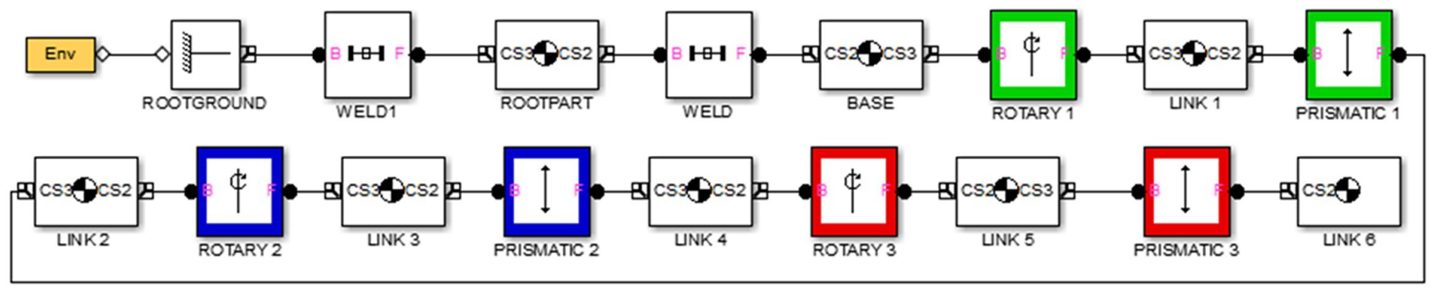
6. Graphic Simulator

This section addresses the development of the redundant planar manipulator robot graphic simulator. Such a simulator is created using the MATLAB/Simulink (including its toolbox SimMechanics™) and Solidworks software, which were chosen due to their 3D modelling and simulation of mechanical system features.

Simmechanics™ Model

Using the SimMechanics Link utility, the CAD assembly developed in SolidWorks is exported to the toolbox SimMechanics™ of MATLAB/Simulink. Then, the SimMechanics toolbox is used to complement and potentiate the basic simulator previously elaborated in SolidWorks. By means of the configuration of blocks representing the components of the redundant planar manipulator robot it is possible to make the robot perform tasks defined by the user, such as controlling its joints and position of its end, among others.

The configuration of some parameters of the blocks is set considering that motion takes place only in the XY plane, and the rest position of the redundant planar manipulator robot occurs when all the links are placed on the X axis, as seen in Figure 2. In home position, it is observed that when each prismatic joint is retracted, the arm and its two forearms are 160 mm long. However, the maximum extension of 200 mm is reached when each prismatic joint is stretched to their limit values, i.e., when each p-joint is extended up to 40 mm the maximum reach of the manipulator is 600 mm long.

Figure 5 shows the circuit in a block diagram imported from the SolidWorks environment, which allows for the dynamic simulation of the redundant manipulator robot. This scheme represents the basic skeleton of the simulator, and was created based on the robot’s real dimensions.

The construction of the manipulator robot considered a structure based on aluminum material.

Table 2. Parameters of the 6-DoF redundant planar manipulator robot links.

Link	Mass (kg)	CG $[\mathit{x};\mathit{y};\mathit{z}]$ (mm)
1	0.4822	[31.7; 0; 442]
2	0.6500	[103.5; 0; 443.1]
3	0.4822	[191.7; 0; 442]
4	0.6500	[263.5; 0; 443.1]
5	0.4822	[351.7; 0; 442]
6	0.6453	[431; 0; 0.442]

presents the main parameters extracted from the blocks modelling each link. These parameters characterize the redundant planar manipulator robot dynamics, with CG as the center of gravity (centroid) measured from the origin of the coordinate system of the respective link.

Among the complementary blocks used in the development of the graphic simulator, those that model actuators and sensors are of great importance, since they generate and record, respectively, all the movements of the redundant planar manipulator robot. In the specific case of actuators, the necessary power signals come from the MATLAB/Simulink environment. Blocks from workspace are used to control each link. These blocks are in charge of reading and storing the diverse joint trajectories programed by the user.

Figure 6 shows the block diagram and connections necessary for simulating and controlling the motion of the first link. Particularly, control is conducted over the first rotary joint of the redundant planar manipulator robot using a method for interpolation through polynomial. Similar connections and control strategies are used to simulate the movement of the remaining links.

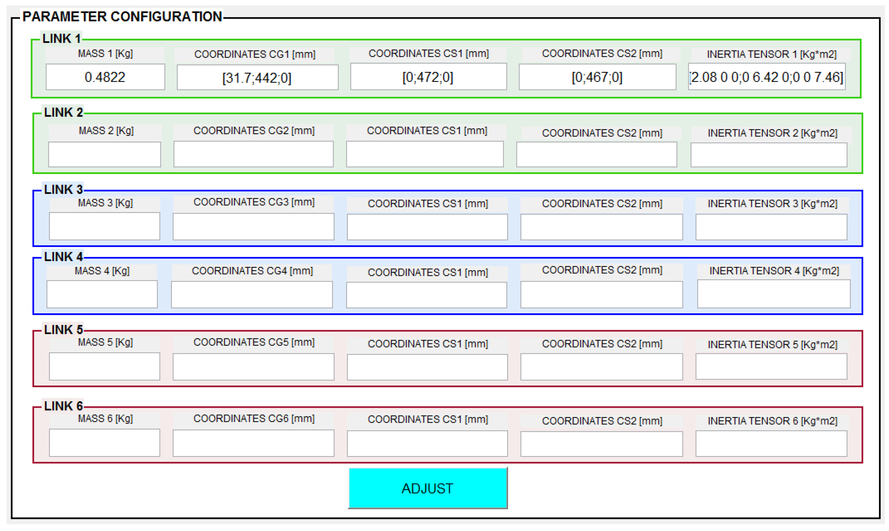
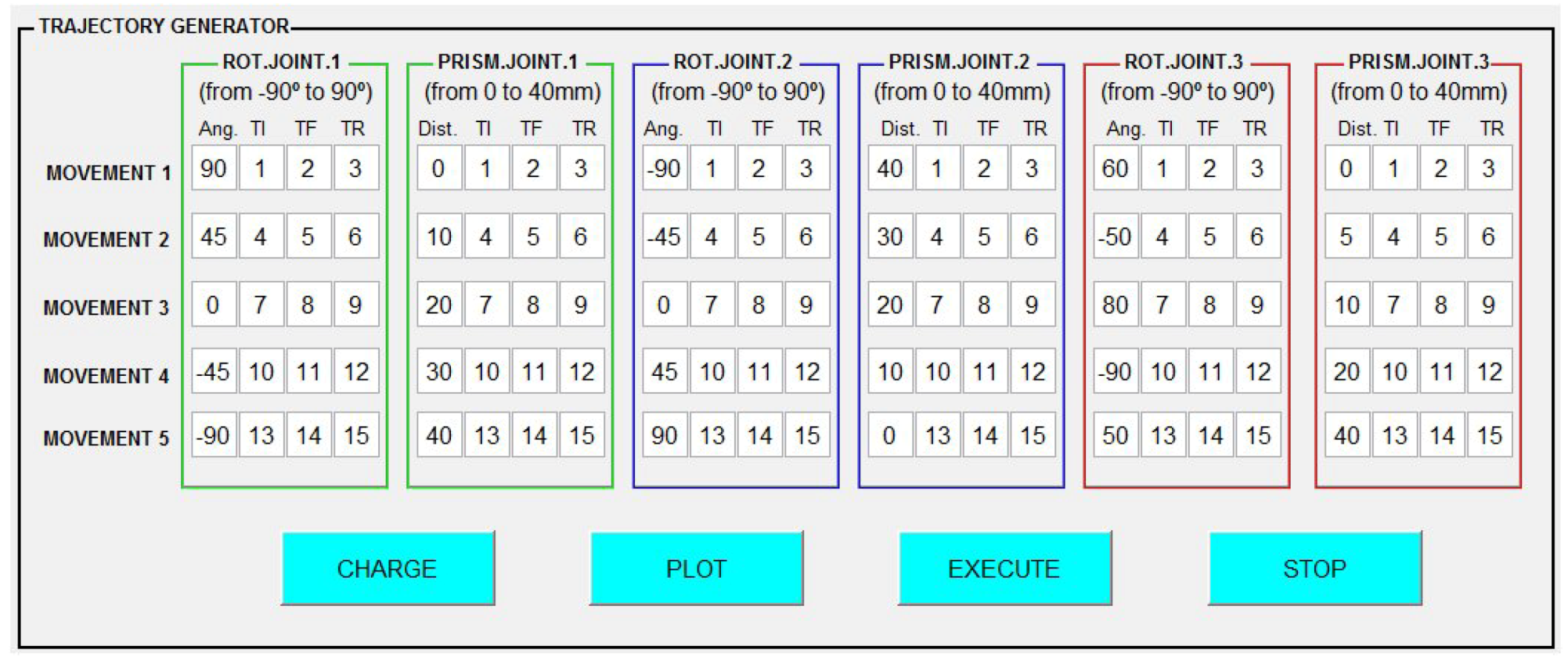
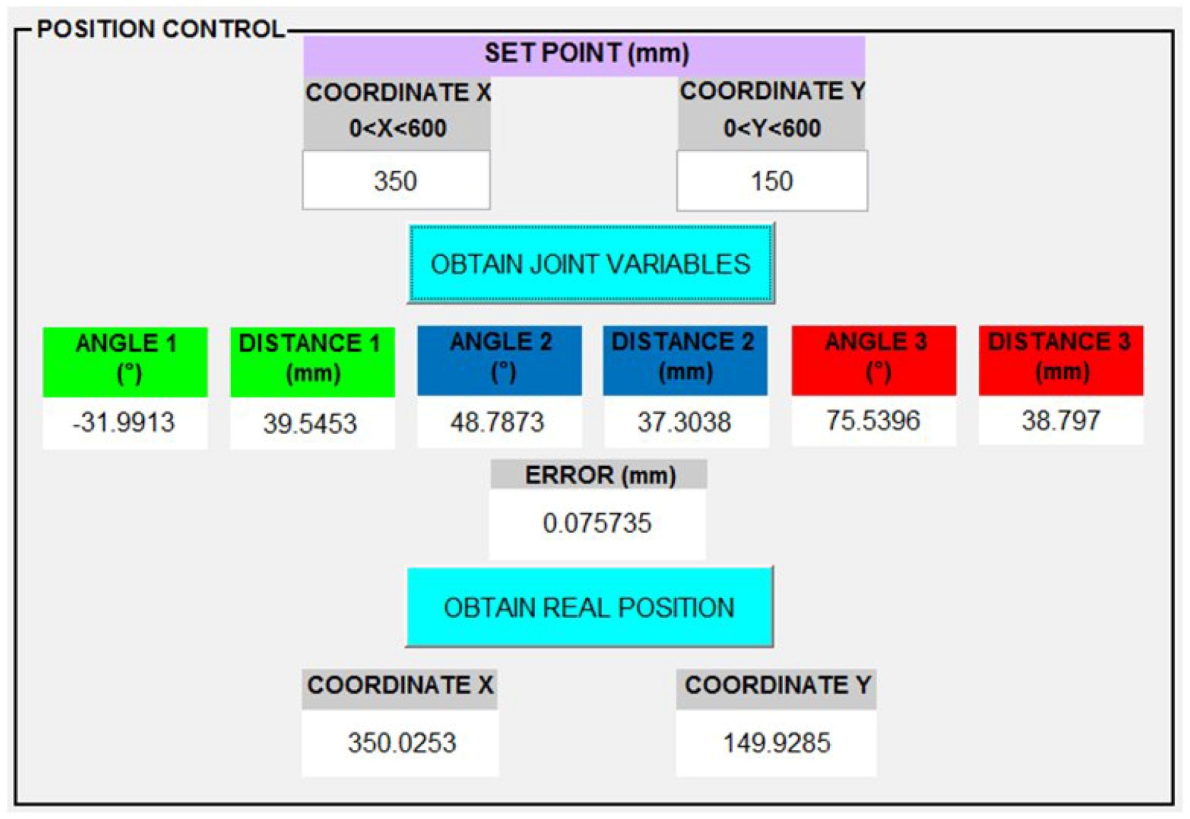
7. Graphic Interface

Below is presented the virtual environment designed to input the parameter values in the blocks that represent the six links that compose the redundant planar manipulator robot. Figure 7 shows, as an example, the configuration window of all the links. Access to this GUIDE in MATLAB is granted through a main window that allows for opening other GUIDE sub-windows. The parameters of the link that can be modified are mass, inertia tensor, position of the center of gravity (CG), and the coordinates of the endpoints of the joints (CS1 and CS2). With this last adjustment, the starting position of each link can be defined and consequently the end effector’s. If any box associated with the link is not configured, the manipulator robot will used the link parameters exhibited by the real manipulator robot in Table 2 by default.

An interpolation method based on polynomial equations is used for controlling the joints of the redundant planar manipulator robot. This is achieved using the pchip instruction of the MATLAB, which allows for constructing third-order polynomials that do not cause overshoot during the movement of the joints, thus making it possible to route and move the joints from their initial positions to the desired positions with few oscillations. Figure 8 shows the GUIDE used to program the following joint trajectories.

This GUIDE allows for entering desired values for the prismatic and rotary joints, indicating also the time of execution (TI), end (TF) and rest (TR) of the movement. The programming limit is five movements per joint. Once the boxes have been filled in using the button “CHARGE”, the values entered are automatically stored in .mat files and in the “from workspace” blocks. Additionally, the trajectories of the programmed joint movements can be visualized through the button “PLOT”, as shown in Figure 9.

The main window of GUIDE also makes it possible to see all the curves resulting from the dynamic performance of the 6-DoF redundant planar manipulator robot, i.e., position, speed, and acceleration of each joint. Specifically, Figure 10 presents the position, speed, and acceleration of the first rotary joint.

Figure 11 shows the development of a GUIDE window, which allows for solving the inverse kinematic problem of the redundant planar manipulator robot based on a SA algorithm. Considering the desired location of the end of the redundant planar manipulator robot, it is possible to know the set of values of the joint variables necessary for reaching this location. The joint variables are six and represent the physical location adopted by the three rotary joints and the three prismatic joints. In addition, the position variables are two, because the end of the robot moves only on the XY plane.

When the coordinates $(x,y)$ are input in the GUIDE window, the workspace allowed to the robot, shown in Figure 12, should be considered, since it depends directly on the mechanical limitations of the same, which are exhibited in

Table 3. Mechanical limitations of the 6-DoF redundant manipulator planar robot joints.

Joint	Range
Rotary 1	$-{90}^{\circ }\le {\theta }_1\le {90}^{\circ }$
Prismatic 1	$0\le d_1\le 40$ (mm)
Rotary 2	$-{90}^{\circ }\le {\theta }_2\le {90}^{\circ }$
Prismatic 2	$0\le d_2\le 40$ (mm)
Rotary 3	$-{90}^{\circ }\le {\theta }_3\le {90}^{\circ }$
Prismatic 3	$0\le d_3\le 40$ (mm)

. The base of the redundant planar manipulator robot is located in the $(x,y)=(0,0)$ coordinate, and its workspace is presented highlighted in blue, with its maximum and minimum scopes being 600 and 160 mm, accordingly, as shown in Figure 12.

By means of the graphic interface, it is possible to enter the coordinates $(x,y)$ of the end effector of the redundant planar manipulator robot; after which, the SA algorithm automatically calculates the inverse kinematics of the same. Figure 11 shows the menu to enter the position. In this example, the coordinate (350,150) yields the solution set with the position adopted by each joint for the entered coordinate. This result corresponds to an inverse kinematics solution selected from multiple options, after 450 iterations of the SA algorithm. Nevertheless, if the coordinates entered are outside its workspace, the SA algorithm automatically adjusts the end of the redundant planar manipulator robot to the closest position within the allowed region, and then delivers the solution set for inverse kinematics.

After continuous simulations for different set points, it is concluded that the SA algorithm requires on average 200 iterations to reach the desired position with an error of 1 mm or less. In addition, with the same number of iterations, the average convergence speed of the algorithm, to make the end effector of the redundant planar manipulator robot move from the initial position to the set point, is 0.5 (s). The scenario changes when the set point is within an unfeasible workspace; in this case, the algorithm needs 2 (s) to take the end effector to an allowed position. The convergence performance of the algorithm strongly depends on the selection of the environmental and cooling parameters defined in Section 6.

8. Conclusions

To characterize the kinematic and dynamic behavior of redundant planar manipulator robots, a graphic simulator was designed and implemented, which allows for entering the Cartesian coordinates $(x,y)$ of the end effector of these robots through a graphic interface, with the purpose of automatically obtaining its inverse kinematics. The basic structure of this basic simulator was built using the software Solidworks, which was subsequently potentiated through the SimMechanics tools of MATLAB/Simulink.

An algorithm based on the probabilistic technique called Simulated Annealing was used for the automatic calculation of the optimal solution, among several options, of the inverse kinematics of the 6-DoF redundant planar manipulator robot. By means of the SA algorithm, it was possible to minimize significantly the distance between any initial position and a target position of the robot’s end effector, reaching values close to zero. In this way, the enhanced algorithm is able to distinguish and correct joints out of the mechanical limits or, also, out of the workspace. In all tests for different targets, the optimization criteria outlined was satisfied (fitness function below or equal 1 mm) and the inverse kinematic solution of the manipulator robot was obtained in a time shorter than one second. This technique can be easily reproduced in other type of manipulator robot configurations with more (or less) redundancy, given that their main component is the information about the direct kinematics, which is easy to obtain in most cases.

To prevent excessive oscillation in the programmed joint trajectories and to ensure the continuity in speed and acceleration of the robot links, the cubic spline interpolation method was used. The dynamic equations were obtained from the L-E equation. Finally, the effectiveness of the methodologies developed was verified through computational simulations of a virtual robot. The results obtained in this study are currently being implemented in the real redundant robot shown in Figure 13.

References

1. Aljalal, M.; Ibrahim, S.; Djemal, R.; Ko, W. Comprehensive review on brain-controlled mobile robots and robotic arms based on electroencephalography signals. Intell. Serv. Robot. 2020. [Google Scholar] [CrossRef]
2. Kim, J.; Cauli, N.; Vicente, P.; Damas, B.; Bernardino, A.; Santos-Victor, J.; Cavallo, F. Cleaning tasks knowledge transfer between heterogeneous robots: A deep learning approach. J. Intell. Robot. Syst. 2020, 98, 191–205. [Google Scholar] [CrossRef] [Green Version]
3. Wang, Z.; Or, K.; Hirai, S. A dual-mode soft gripper for food packaging. Robot. Auton. Syst. 2020, 125, 103427. [Google Scholar] [CrossRef]
4. Iqbal, H.; Khan, M.U.A.; Yi, B.-J. Analysis of duality-based interconnected kinematics of planar serial and parallel manipulators using screw theory. Intell. Serv. Robot. 2020, 13, 47–62. [Google Scholar] [CrossRef]
5. Kern, J.; Jamett, M.; Urrea, C.; Torres, H. Development of a neural controller applied in a 5-DoF robot redundant. IEEE Lat. Am. Trans. 2014, 12, 98–106. [Google Scholar] [CrossRef]
6. Le, Q.D.; Kang, H.-J. Finite-time fault-tolerant control for a robot manipulator based on synchronous terminal sliding mode control. Appl. Sci. 2020, 10, 2998. [Google Scholar] [CrossRef]
7. Cieślak, P.; Simoni, R.; Ridao Rodríguez, P.; Youakim, D. Practical formulation of obstacle avoidance in the task-priority framework for use in robotic inspection and intervention scenarios. Robot. Auton. Syst. 2020, 124, 103396. [Google Scholar] [CrossRef]
8. Shanda, W.; Xiao, L.; Qingsheng, L.; Baoling, H. Existence conditions and general solutions of closed-form inverse kinematics for revolute serial robots. Appl. Sci. 2019, 9, 4365. [Google Scholar] [CrossRef] [Green Version]
9. Fan, S.; Xie, X.; Zhou, X. Optimum manipulator path generation based on improved differential evolution constrained optimization algorithm. Int. J. Adv. Robot. Syst. 2019, 16, 1729881419872060. [Google Scholar] [CrossRef]
10. Shafei, A.M.; Mirzaeinejad, H. A general formulation for managing trajectory tracking in non-holonomic moving manipulators with rotary-sliding joints. J. Intell. Robot. Syst. 2020. [Google Scholar] [CrossRef]
11. Rahmani, M.; Rahman, M.H. Adaptive neural network fast fractional sliding mode control of a 7-DOF exoskeleton robot. Int. J. Control Autom. Syst. 2020, 18, 124–133. [Google Scholar] [CrossRef]
12. Bobrow, J.E.; Martin, B.; Sohl, G.; Wang, E.C.; Park, F.C.; Kim, J. Optimal robot motions for physical criteria. J. Robot. Syst. 2001, 18, 785–795. [Google Scholar] [CrossRef]
13. López-Franco, C.; Hernandez-Barragan, J.; Alanis, A.Y.; Arana-Daniel, N. A soft computing approach for inverse kinematics of robot manipulators. Eng. Appl. Artif. Intell. 2018, 74, 104–120. [Google Scholar] [CrossRef]
14. Li, T.; Zheng, S.; Shu, X.; Wang, C.; Liu, C. Self-recognition grasping operation with a vision-based redundant manipulator system. Appl. Sci. 2019, 9, 5172. [Google Scholar] [CrossRef] [Green Version]
15. Qian, Y.; Yuan, J.; Wan, W. Improved trajectory planning method for space robot-system with collision prediction. J. Intell. Robot. Syst. 2020, 99, 289–302. [Google Scholar] [CrossRef]
16. Teja, H.; Shah, S. Learning inverse kinematic solutions of redundant manipulators using multiple internal models. In Proceedings of the 6th IEEE International Conference on Biomedical Robotics and Biomechatronics (BioRob), Utown, Singapore, 26–29 June 2016; p. 1371. [Google Scholar]
17. Zhao, R.; Shi, Z.; Guan, Y.; Shao, Z.; Zhang, Q.; Wang, G. Inverse kinematic solution of 6R robot manipulators based on screw theory and the Paden-Kahan subproblem. Int. J. Adv. Robot. Syst. 2018, 15, 1–11. [Google Scholar] [CrossRef]
18. Bai, L.; Yang, J.; Chen, X.; Jiang, P.; Liu, F.; Zheng, F.; Sun, Y. Solving the time-varying inverse kinematics problem for the Da Vinci surgical robot. Appl. Sci. 2019, 9, 546. [Google Scholar] [CrossRef] [Green Version]
19. Huang, Q.; Nie, L. A fast convergence efficiency method of inverse kinematics for robot manipulators. J. Appl. Sci. 2013, 13, 5174–5179. [Google Scholar] [CrossRef] [Green Version]
20. Park, S.-O.; Lee, M.C.; Kim, J. Trajectory planning with collision avoidance for redundant robots using jacobian and artificial potential field-based real-time inverse kinematics. Int. J. Control Autom. Syst. 2020, 18, 2095–2107. [Google Scholar] [CrossRef]
21. Besset, P.; Taylor, C.J. Inverse kinematics for a redundant robotic manipulator used for nuclear decommissioning. In Proceedings of the UKACC International Conference on Control (CONTROL), Loughborough, UK, 9–11 July 2014; pp. 56–61. [Google Scholar]
22. Farzan, S.; DeSouza, G.N. A parallel evolutionary solution for the inverse kinematics of generic robotic manipulators. In Proceedings of the IEEE Congress on Evolutionary Computation (CEC), Beijing, China, 6–11 July 2014; pp. 358–365. [Google Scholar]
23. Köker, R.; Cakar, T. A neuro-genetic-simulated annealing approach to the inverse kinematics solution of robots: A simulation based study. Eng. Comput. 2016, 32, 553–565. [Google Scholar] [CrossRef]
24. López-Franco, C.; Hernández-Barragán, J.; Alanis, A.Y.; Arana-Daniel, N.; López-Franco, M. Inverse kinematics of mobile manipulators based on differential evolution. Int. J. Adv. Robot. Syst. 2018, 15, 1–22. [Google Scholar] [CrossRef] [Green Version]
25. Dereli, S.; Köker, R. Simulation based calculation of the inverse kinematics solution of 7-DOF robot manipulator using artificial bee colony algorithm. SN Appl. Sci. 2020, 2, 27. [Google Scholar] [CrossRef] [Green Version]
26. Zhou, Z.; Guo, H.; Wang, Y.; Zhu, Z.; Wu, J.; Liu, X. Inverse kinematics solution for robotic manipulator based on extreme learning machine and sequential mutation genetic algorithm. Int. J. Adv. Robot. Syst. 2018, 15, 1–15. [Google Scholar] [CrossRef]
27. Song, B.; Wang, Z.; Zou, L.; Xu, L.; Alsaadi, F.E. A new approach to smooth global path planning of mobile robots with kinematic constraints. Int. J. Mach. Learn. Cybern. 2019, 10, 107–119. [Google Scholar] [CrossRef]
28. Kereluk, J.A.; Emami, M.R. A new modular, autonomously reconfigurable manipulator platform. Int. J. Adv. Robot. Syst. 2015, 12, 1–17. [Google Scholar] [CrossRef]
29. Truong, L.V.; Huang, S.D.; Yen, V.T.; Cuong, P.V. Adaptive trajectory neural network tracking control for industrial robot manipulators with deadzone robust compensator. Int. J. Control Autom. Syst. 2020, 1–12. [Google Scholar]
30. Bjerkeng, M.; Pettersen, K.Y. A new Coriolis matrix factorization. In Proceedings of the IEEE International Conference on Robotics and Automation, Saint Paul, MN, USA, 14–18 May 2012; pp. 4974–4979. [Google Scholar]
31. Zarrin, A.; Azizi, S.; Aliasghary, M. A novel inverse kinematics scheme for the design and fabrication of a five degree of freedom arm robot. Int. J. Dyn. Control 2020, 8, 604–614. [Google Scholar] [CrossRef]
32. Segota, S.B.; Andelic, N.; Lorencin, I.; Saga, M.; Car, Z. Path planning optimization of six-degree-of-freedom robotic manipulators using evolutionary algorithms. Int. J. Adv. Robot. Syst. 2020, 17, 1–16. [Google Scholar]
33. García-Ródenas, R.; López-García, M.L.; Sánchez-Rico, M.T.; López-Gómez, J.A. A bilevel approach to enhance prefixed traffic signal optimization. Eng. Appl. Artif. Intell. 2019, 84, 51–65. [Google Scholar] [CrossRef]
34. Bi, H.; Lu, F.; Duan, S.; Huang, M.; Zhu, J.; Liu, M. Two-level principal–agent model for schedule risk control of IT outsourcing project based on genetic algorithm. Eng. Appl. Artif. Intell. 2020, 91, 103584. [Google Scholar] [CrossRef]
35. Ileri, Y.Y.; Hacibeyoglu, M. Advancing competitive position in healthcare: A hybrid metaheuristic nutrition decision support system. Int. J. Mach. Learn. Cybern. 2019, 10, 1385–1398. [Google Scholar] [CrossRef]
Figure 1. Geometrical configuration of the 6-DoF redundant planar manipulator robot and assignation of the D-H coordinate system (perspective view).
Applsci 10 06770 g001
Figure 2. Resting location and position of the mass centers of the 6 links.
Applsci 10 06770 g002
Figure 3. Cost function associated with the x i and x j vectors.
Applsci 10 06770 g003
Figure 4. SA algorithm flowchart.
Applsci 10 06770 g004
Figure 5. Basic simulation circuit for the 6-DoF redundant planar manipulator robot.
Applsci 10 06770 g005
Figure 6. Control loop of the first rotary joint of the 6-DoF redundant planar manipulator robot.
Applsci 10 06770 g006
Figure 7. Configuration of the 6-DoF redundant planar manipulator robot parameters.
Applsci 10 06770 g007
Figure 8. GUIDE for programming trajectories.
Applsci 10 06770 g008
Figure 9. Visualization of the programmed joint trajectories.
Applsci 10 06770 g009
Figure 10. Dynamic performance curves of the first rotary joint. Position, speed, and acceleration.
Applsci 10 06770 g010
Figure 11. GUIDE window for obtaining the values of the joint variables.
Applsci 10 06770 g011
Figure 12. Workspace of the 6-DoF redundant planar manipulator robot.
Applsci 10 06770 g012
Figure 13. Real redundant planar manipulator robot.
Applsci 10 06770 g013