BassNet: A Variational Gated Autoencoder for Conditional Generation of Bass Guitar Tracks with Learned Interactive Control


1
Contractor for Sony Computer Science Laboratories, 75005 Paris, France
2
Sony Computer Science Laboratories, 75005 Paris, France
*
Author to whom correspondence should be addressed.
Appl. Sci. 2020, 10(18), 6627; https://doi.org/10.3390/app10186627
Submission received: 1 August 2020
/
Revised: 31 August 2020
/
Accepted: 17 September 2020
/
Published: 22 September 2020
(This article belongs to the Special Issue Deep Learning for Applications in Acoustics: Modeling, Synthesis, and Listening)
Abstract
:Deep learning has given AI-based methods for music creation a boost by over the past years. An important challenge in this field is to balance user control and autonomy in music generation systems. In this work, we present BassNet, a deep learning model for generating bass guitar tracks based on musical source material. An innovative aspect of our work is that the model is trained to learn a temporally stable two-dimensional latent space variable that offers interactive user control. We empirically show that the model can disentangle bass patterns that require sensitivity to harmony, instrument timbre, and rhythm. An ablation study reveals that this capability is because of the temporal stability constraint on latent space trajectories during training. We also demonstrate that models that are trained on pop/rock music learn a latent space that offers control over the diatonic characteristics of the output, among other things. Lastly, we present and discuss generated bass tracks for three different music fragments. The work that is presented here is a step toward the integration of AI-based technology in the workflow of musical content creators.
1. Introduction
The advent of machine learning has unlocked a wealth of possibilities for innovation in music creation, as in many other areas. Although applications of artificial intelligence (AI) techniques in music creation have been around for more than half a century [1,2], deep learning has renewed interest in computer-driven and computer-assisted forms of music creation.
A common approach for music creation using AI is to train a generative probabilistic model of the data [3,4,5] and create music by iterative sampling, possibly while using constraints [6,7]. More recently, deep learning applications in music creation have focused on generating waveforms directly [8], often using techniques that have been adopted from speech synthesis.
In many of the above approaches, the opportunities for user control and interactive human–computer creation are limited or inconvenient (some exceptions are [9,10]). Apart from imposing constraints, as mentioned above, a common way of exercising control over the output of models for music creation is to provide conditioning signals, based on which the output is generated. It is useful to distinguish between dense conditioning signals, such as an audio track, and sparse conditioning signals, such as a category label. The former typically provide rich information from which the structure shape of the output is inferred. The latter only give a hint as to the character of the desired output, but leave the specific structure and shape unspecified.
This dichotomy highlights an important issue for AI in music creation. With dense conditioning signals, models can generally create higher quality output, and can possibly be more precisely controlled, but dense conditioning signals are impractical as a means of control from a user perspective. Sparse conditioning signals, on the other hand, are much easier to provide and manipulate by a user, but the quality of the output is generally lower, and it is hard to use such signals for fine-grained control of the output.
From a creative perspective, an important issue with models that create outputs to accompany existing musical material (typically by providing the existing material as a dense conditioning signal) is how to honor the notion of artistic license. To human musicians, playing along with existing musical material constrains what they play, but by no means fully determines it, which leaves room for a variety of possibilities. For instance, given a chord progression and/or drum rhythm, bass players may choose to play different accompanying bass lines, depending on their taste, capabilities, and musical intentions. Whereas, some possible bass lines may serve to consolidate the existing rhythmical structure by playing harmonically stable notes on metrically stable positions in the music, others may enrich the existing material by playing in a more contrapuntal manner. Bass players may also choose to align their bass line more closely to a particular instrument that is present in the existing material.
In this paper, we present BassNet, which is a deep learning approach that combines both dense and sparse conditioning signals to generate bass guitar accompaniments for one or more input audio tracks. The input tracks may contain rhythmical and harmonic parts, such as guitar, keyboards, and drums, and provide the dense conditioning signal. A second, sparse conditioning signal is provided to the model in the form of a (possibly time-varying) two-dimensional (2D) coordinate that the user can freely choose to control the character of the generated bass guitar accompaniments.
A distinctive feature of the proposed approach with respect to most work on conditional music generation is that the sparse conditioning signal is unsupervised, rather than supervised. Another notable characteristic of our approach is that the sparse conditioning signal is designed to control the relationship between the generated output and the dense conditioning signal (the input tracks), rather than the qualities of the generated output itself. Thus, instead of the dense and sparse conditioning signals independently competing for influence over the output, the sparse conditioning signal is designed to modulate the influence of the dense conditioning signal on the output. This design decision follows from the intuition that the generated bass track—as deviant as it may be from the input tracks—should be construed in relation to, and not independently of, the input tracks.
To our knowledge, BassNet (along with the related DrumNet system, see Section 3 for commonalities and differences) is the first conditional music generation system to use the latent space in this modulating role. A further important contribution of this paper is a demonstration that imposing temporal stability on latent space trajectories during training (using cross-reconstruction loss) tends to lead to disentangled latent representations of bass patterns.
In this paper we describe the BassNet architecture and a procedure for training the model (Section 4). We start with an overview of the background work on which our work is based (Section 2), and a discussion of related work in the field of conditional music generation (Section 3). In Section 5, we define an experimental setup to validate the approach by examining the capabilities of the model to organize the learned 2D control space according to latent patterns in artificial datasets. We perform further evaluation by training the BassNet architecture on real world data, and investigating the effect of the 2D control space on the pitch distribution of the generated bass tracks. We pay special attention to the effect of the temporal window size of the data on the performance of the model, as well as the effect of the imposing a temporal stability constraint on latent space trajectories during training. The results of this experimentation are presented and discussed in Section 6. In this section, we also present case studies, in which we discuss different model outputs for a given musical fragment. Section 7 presents conclusions and future work.
2. Background
Autoencoders learn (compressed) latent representations of data instances while using an encoder/decoder architecture, where the training objective is to simply reconstruct the input given latent encoding. The dimensionality of the latent space is usually smaller than that of the input in order not to learn trivial representations. Other ways to learn meaningful, compressed representations of the data in autoencoders are to employ sparsity regularization in the latent space, or to corrupt the input, for example, with dropout [11]. As the distribution of the latent space is not known in general, there exists no efficient way to sample from common autoencoders. The possible ways to impose a prior on the latent space consist of using auxiliary losses, like in Adversarial Autoencoders [12], or by sampling directly from parametric distributions, like in Variational Autoencoders [13] (VAEs). When the prior is known, it is possible to draw samples from the model, and to manually explore the latent space in order to better control the model output.
A particular form of autoencoders are Gated Autoencoders (GAEs) [14,15], which, instead of learning latent representations of the data, aim to learn transformations between pairs of data points. While the term “gating” in neural networks often refers to “on/off switches” using sigmoid non-linearities, Gated Autoencoders follow a different paradigm. Instead, they are a form of bi-linear (two-factor) models, whose outputs are linear in either factor when the other is held constant. The resulting factors can then be encoded while using any typical autoencoder-like architecture, leading to latent spaces that represent transformations between data pairs. Besides vanilla GAEs [16] (resembling de-noising autoencoders), other variants exists, like Gated Boltzmann Machines [17,18], Gated Adversarial Autoencoders [19], or Variational Gated Autoencoders (this work). The mathematical principle of GAEs is to learn the complex eigenvectors of orthogonal transformations in the data, as has been made explicit in [20]. However, prior work has empirically shown that the assumption of orthogonality in the learned transformations can be loosened by using non-linearities in layer outputs, as well as predictive training (instead of symmetric reconstruction) [19,21].
Another interesting feature of GAEs are that they are particularly suited for learning invariances to specific transformations when those transformations are applied to input and output simultaneously. For example, local time-invariance in sequence modeling leads to temporal stability of latent representations [19], and transposition-invariance in music leads to representations of musical intervals [21]. This learning of invariances, specifically of temporally stable features using the eigenvectors of transformations, comprises an distinct line of research, which is also known as slow feature analysis [20,22,23,24]. A GAE can be thought of as putting an additional neural network stack on top such slow features in order to learn feature combinations, which improves the robustness and expressivity of the architecture as a whole, and it is also advantageous for the invariance learning itself.
3. Related Work
At the present time, we can look back to an ever growing number of works that are related to symbolic music and audio generation. In earlier contributions, the main focus was on symbolic music generation, using RNNs [9,25,26,27], Restricted Boltzmann Machines [7], or combinations of both [4,28,29]. More recent works use GANs [30,31,32] and Transformer architectures [33,34] for symbolic music generation. Through advances in hardware performance, it became possible to directly generate audio waveforms with neural networks. The first examples of this approach are the well-known WaveNet architecture [35], but also GAN-based approaches, like GANSynth [36] or WaveGAN [37] and, most recently, with JukeBox [5], a very elaborate Transformer model showed that it is possible to generate full songs in the audio domain.
In music production, it is relevant for a user how to control such music generation models. Obviously, latent spaces are well-suited for exploration, and models that possess such latent spaces (e.g., VAEs and GANs) are directly applicable to such user control [38,39,40,41]. Typically, additional conditional signals are provided during training, in a supervised manner. At generation time, this conditional signal can be varied as a means of user control over the generated output. Along this line, models for audio synthesis have been conditioned on pitch information [36,38], categorical semantic tags [42], lyrics [5], or on perceptual features [43,44]. Other approaches use conditioning in symbolic music generation [45], or constraints during generation instead of conditional information during training [7,46]. Note the difference of these approaches with the approach presented here, in which the latent space itself is designed to be usable as a user control.
The general approach that is taken in this paper is closely related to that of the GAE-based DrumNet [19]. However, DrumNet only operates on one-dimensional sequences of onset functions, while BassNet uses spectro–temporal representations. Additionally, DrumNet uses an adversarial autoencoder architecture to represent the input/output relations, while BassNet uses a VAE-approach. In most models where the latent space can be controlled by a user, possible additional supervised conditioning information is usually sparse (e.g., pitch information, perceptual features, lyrics, or semantic tags). GAEs, on the other hand, naturally provide a conditioning on some dense context (e.g., audio input in CQT representation), and a user-controllable feature space. Other works where GAEs have been used for music modeling include common GAEs for learning transformations of musical material [47], predictive GAEs for learning musical intervals from data [21], and recurrent GAEs for music prediction [48].
Outside of the musical domain, GAEs have been used to learn transformation-invariant representations for classification tasks [15], for parent-offspring resemblance [49], for learning to negate adjectives in linguistics [50], for activity recognition with the Kinekt sensor [51], in robotics to learn to write numbers [52], and for learning multi-modal mappings between action, sound, and visual stimuli [53]. In sequence modeling, GAEs have been utilized in order to learn co-variances between subsequent frames in movies of rotated three-dimensional (3D) objects [16] and to predict accelerated motion by stacking more layers in order to learn higher-order derivatives [54].
4. The Bassnet Model
The BassNet model architecture and information flow is shown in Figure 1. The architecture is designed to model the relationship between a mono mix of one or more input tracks (henceforth referred to as the mix), and a mono output track containing the bass. The mix and bass are represented as CQT magnitude spectrograms (see Section 4.1), denoted x and y, respectively. Although the architecture involves convolution along both the frequency and the time axes, the inputs to the model are fixed length windows of the spectrograms, rather than the spectrograms of the entire tracks.
The relationship between x and y is encoded in a latent variable z, as shown in the upper half of the diagram in Figure 1. The latent variable can be of arbitrary dimensionality, but, in the present work, we use a fixed dimensionality of two, so that it can be conveniently presented to the user without dimensionality reduction. Although the x and y variables convey windows of multiple timesteps, the corresponding z is just a single coordinate in the latent space. As such, the value of z (i.e., a pair of real-valued scalars) describes the constellation of spectro-temporal relationships between x and y, not just spectral relationships at a single timestep.
Because the modeling of the relationship between the mix and the bass is done while using CQT magnitude spectra, rather than using waveforms, we need an extra sonification step to convert the model outputs into an audio track. We do this by inferring three low-level audio descriptors from the generated magnitude spectrogram , from which a bass track is then synthesized. This process corresponds to the lower right part of the diagram. The lower left part depicts the extraction of descriptors from the data in order to serve as ground truth in the training phase.
In the rest of this section, we describe the various aspects of the architecture in more detail. We start with a brief discussion of the input representation (Section 4.1). Subsequently, we give an overview of the audio descriptors for the bass track (Section 4.2). We then focus on the GAE part of the architecture, and formulate a training objective to produce temporally stable latent representations (Section 4.4).
4.1. Model Input: CQT Log Magnitude Spectrograms
The BassNet model works with spectral representation of audio data. The monaural mix and bass signals are converted to the spectral domain while using the Constant-Q Transform (CQT), a non-invertible audio transform [55] that is often used in music applications because of its logarithmic frequency scale, which allows for the frequency bins to coincide with the chromatic scale.
As is common in music applications, we discard phase information from the CQT and only use its magnitude. Furthermore, we anticipate that the pitch—and therefore the harmonics—of the mix and bass will play an important role in learning relations between the two. Because of this, we choose a relatively high frequency resolution for the CQT, computing 36 frequency bins per octave (three bins per semitone), over a range of 88 semitones, starting from 27.5 Hz (the pitch A0), yielding 264 frequency bins in total. Because higher harmonics of musical sounds often have low energy as compared to the lower harmonics, we take the log of the CQT magnitude spectrogram, so that the overtone structure of sounds is emphasized. For computing the CQTs, we use an adaptation of the CQT implementation of the nnAudio library [56]. Before computing the CQTs, we resample the mono mixes at 16 KHz. The CQT spectrograms have a hop time of 0.01 s.
4.2. Extraction of Audio Descriptors
The sonification of CQT log magnitude spectrogram outputs generated by the model is not straight-forward, because this data representation is not lossless. First of all, the phase information is discarded and, furthermore, the CQT transform is not invertible, like, for instance, the Fast Fourier Transform. However, because we need to sonify only data describing a single source type (bass guitar), and assuming the bass guitar tracks are monophonic, it is often possible to create a rough approximation of the target sound while using some form of additive synthesis based on a small set of audio descriptors.
In the current work, we use pitch (or fundamental frequency, denoted ), level (denoted l), and onset strength (denoted o) as descriptors for sonification. Here, we define level as the instantaneous power of the STFT spectrogram, expressed in dB. These descriptors capture aspects of the sound that can be estimated from the CQT spectrogram relatively accurately and, at the same time, provide—in the case of monophonic bass guitar—sufficient information to synthesize a bass sound.
We need ground truth data to train the model to predict these descriptors from the generated CQT spectrogram . To extract instantaneous pitch values from the bass tracks in the training data we the convolutional neural network (CNN) pitch estimation system crepe [57]. For onset strength, we use the CNN onset detector from madmom [58,59]. Both are publicly available state-of-the-art methods. To estimate sound level we use the stft and power_to_db functions from librosa [60].
4.3. Temporal Multi-Resolution
The amount of computer memory that is needed to pass data and gradients through the model is proportional to the window size, and large window sizes may have prohibitive memory requirements. To accommodate for larger window sizes, we use what we call temporal multi-resolution, a lossy compression of the data into multiple channels of smaller size than the original data. This technique consists in repeated downsampling and cropping of data windows along the time axis with increasing downsample ratios, in such a way that the data in the center of the window are kept at full resolution, and the data are stored with decreasing resolution towards the outer parts of the window. The data at different resolutions are cropped in such a way that the results have equal length, and can thus be stored alongside each other as separate channels in a tensor. Figure 2 illustrates the process.
Note that the total number of elements in the compressed data window scales logarithmically with the number of elements in the original data window. The example presented in Figure 2 yields a modest reduction from 16 elements to 12 elements, but note that following the same procedure a window of 128 elements is compressed to 24 elements. Furthermore, note that the compressed window size can be varied. In the given example, it is set at 4, which for an input of size 16 yields channels. A compressed window size of 2 would encode an input size 16 into channels, and compressed size of 8 would yield channels. When specifying the window size in a multi-resolution setup we specify both the compressed and the expanded (i.e., original) window size. For example, the multi-resolution window in Figure 2 would be specified as 4/16.
The expansion step that is shown at the bottom of Figure 2 is used for combining the outputs of the model for consecutive windows. We expand the compressed window by upsampling the downsampled channels and substituting the center part of the upsampled data by the data of the higher resolution data. The expanded data are then windowed and used in an overlap-and-add fashion in order to produce a full track (not shown in the figure). We use an even-sized non-symmetric Hann window, because it allows for adding overlapped windows without rescaling when using a hop size of half the window size. The impact of the low-resolution parts of the expanded window is limited, because the windowing weights the center of the windows stronger than the sides.
4.4. Learning Latent Representations to Encode the Relationship between X and Y
The relationship between the multi-resolution CQT log magnitude spectrograms x and y is modeled while using a Variational Gated Autoencoder (VGAE), shown in the upper part of Figure 1. It differs from the standard GAE, in that the latent variable z (also called mapping) has a stochastic interpretation, as in VAEs. The conversion of the modeled variables x, y, and z to and from the factors (the intermediate representations that are multiplied in a pairwise fashion) is performed by the encoder–decoder pairs /, /, and /, respectively.
In the next Subsection (Section 4.4.1), we describe the implementation of the encoder/decoder pairs, and we will then formulate a training objective for the architecture that enforces the temporal stability of the latent variable.
4.4.1. Encoder/Decoder: Stacked Dilated Residual Blocks
Dilated residual networks [61] combine dilated convolution and additive skip connections in stackable units, referred to as dilated residual blocks. The dilated convolution allows for large receptive fields in higher layers without the need for large kernels, strides, or pooling. This means that high level features can be represented at the same resolution as the input itself. The additive skip connections are a solution to the problem that the gradient of the loss in traditional deep networks tends vanish in the lower layers of the network, which limits maximal depth at which networks can be effectively trained [62]. Dilated residual networks have proven to be especially successful in tasks with dense targets, like image segmentation, and object localization [61], as well as stereo-image depth estimation [63].
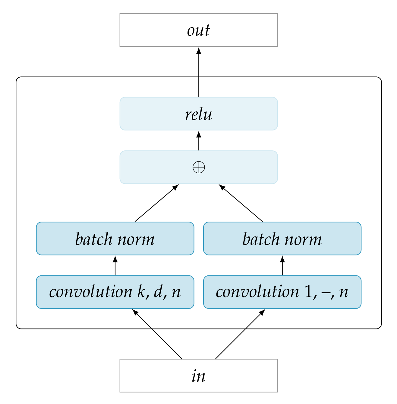
In this work, we use an adaptation of the dilated residual block proposed in [61] as the building block for the encoders and decoders. Figure 3 depicts the block. In this structure, the information flows from input to output through two pathways in parallel. The left pathway involves a typical convolution layer with configurable parameters: the kernel size k, number of kernels n, and dilation factor d. The right pathway convolution uses kernels of size 1 (dilation does not apply in this case) and, thus, does not compute any features from the input. Instead, it outputs n linear combinations of the input to ensure shape compatibility for elementwise addition to the n feature maps of the left pathway. The pathways further include batch normalization operations. After the elementwise sum of the pathways, a rectified linear unit allows for a non-linear response.
A practical advantage of the residual blocks as used here is that the shape of the output is identical to the shape of the input, due to the fact that the convolution stride is always 1 and there is no pooling operator. Thus, residual blocks can be stacked very simply to obtain deeper architectures.
The encoders and decoders in the current architecture are identical, except for the fact that the decoders use transposed convolution. The weights between the encoder convolutions and decoder transposed convolutions are tied.
4.4.2. Training Objective
The left side of the VGAE—which is denoted as /, colored green in Figure 1—encodes x and y to the parameters and of a gaussian distribution over the latent space Z. Conversely, given x, the right side of the VGAE—denoted as , colored purple—decodes a sample to a reconstruction of y, being denoted :
where are CQT spectrogram windows, comprising T timesteps, C channels, and F frequency bins.
Standard VAE Training Objective
The standard VAE learning objective includes two terms in the loss function to be minimized: (1) the Kullback–Leibler divergence between the conditional distribution and the standard multivariate normal distribution and (2) the negative log-likelihood of the data. Interpreting the real-valued decoded model output as the mean of an isotropic gaussian distribution , which minimizes the negative log-likelihood of the data is equivalent to minimizing the mean squared error MSE between the data y and its reconstruction [64] [Section 6.2.2.1], so the objective can be written as:
Enforcing Temporal Stability in Latent Representations
Note that, in our current setting, where there is a temporal ordering on data instances (i.e., consecutive spectrogram windows), this learning objective does not pose any constraint on the evolution of z through time. Thus, z may be trained to encode aspects of the relation between x and y that vary strongly through time. The intuition underlying slow feature analysis (Section 2) that the semantically relevant aspects of time series tend to remain stable over time suggests that the learning objective should be modified in order to enforce the temporal stability of z.
To this aim, we propose to modify/extend both the divergence and reconstruction loss terms in while using the notion of cross-reconstruction. Cross-reconstruction has been used in different settings, for example, for multimodal clustering [65], zero-shot learning [66], and learn transformation invariant representations [67]. In the current context, we implement cross-reconstruction as follows: For a given instance , we select a second instance at random from the temporal vicinity of . Using the equations, we compute the cross-reconstructions and :
Minimizing the cross-reconstruction loss terms and encourages the robustness of the decoding step against the variability of z within a temporal neighborhood, but it does not necessarily enforce the stationarity of z within the neighborhood. The latter can be achieved by minimizing what we call the cross-divergence loss: the Kullback–Leibler divergence between and .
Adding the cross-divergence loss and replacing the reconstruction loss term in Equation (5) by the cross-reconstruction loss terms, we obtain the following loss function for an instance :
where is a randomly selected instance from the temporal neighborhood of .
Reconstruction Loss Terms for Descriptors
The above loss function is aimed at producing a temporally stable latent space that learns relationships between the CQT log magnitude spectrograms x and y. Because, in addition to producing a , we want the model to predict the pitch, level, and onset audio descriptors, we add the corresponding loss terms. For pitch, the output of the model is a categorical distribution over the center frequencies of the 264 CQT bins, and for the level and onset descriptors the output is a Bernoulli distribution. Accordingly, we extend from Equation (8) with the categorical cross-entropy (CCE) loss for the pitch predictions, and the binary cross-entropy (BCE) loss for level and onset:
We do not use the cross-reconstruction loss with a randomly selected neighbor, but rather the reconstruction loss of itself, in order to have a deterministic loss criterion for validation and testing:
5. Experimental Setup
In this section, we report the experimentation that we first carried out to test the effectiveness of the approach empirically, and secondly to investigate the characteristics and consistency of the mappings that the model learns between the mix and the bass on a corpus of pop/rock songs. As in any modeling approach involving deep learning, there are many hyper-parameters and training specifics to be configured and some of these settings may have a large impact on performance. Although an exhaustive evaluation of all settings is beyond the scope of this paper, we do evaluate the effect of the window size on the performance of the model. For other settings, we use values that we found to work well on an ad-hoc basis during the development of the approach. These settings may be subject to further optimization.
The trained models are evaluated in terms of the cross-entropy loss with respect to the pitch, onset, and level descriptors, which provides a measure of how well the models perform as generative models of the data.
Furthermore, we interpret the effectiveness of the approach in terms of its capability to identify patterns between the mix and the bass and to learn a disentangled representation of the patterns in the latent space. This requires ground truth knowledge of the relationships between the mix and the bass and, to this end, we train the model on a number of artificially created datasets. Each of the datasets is designed in order to test the sensitivity of the model to a different aspect of the input, such as instrument timbre, harmony, and rhythm. We evaluate the results by way of a quadratic discriminant analysis on the latent space, which quantifies the degree to which the patterns are disentangled.
Subsequently we train models of different window sizes on a dataset of commercial pop/rock songs. In this case, we analyze the results by comparing the statistics of predicted pitch and onset values to the statistics of ground truth pitch and onset values, and discussing how these statistics change when the latent variable is changed. Lastly, we show some concrete examples that illustrate how, for a given mix, different variations of the bass can be created by varying the latent variable.
In the remainder of this section, we describe the datasets used and report the specifics of the model training procedure.
5.1. Artificial Datasets
We define four artificial datasets, each comprising 1000 pairs of mix and bass audio tracks. The audio tracks are created by synthesizing programmatically created MIDI tracks, while using the publicly available FluidR3_GM soundfont. The characteristics of the mix tracks are mostly identical across the four datasets (with two exceptions explained below). The difference between the datasets is in the way the bass track is related to the mix track. In each dataset, we define two or more bass patterns that specify what the bass plays in function of the mix (chords and drums). The bass track is generated from the mix track measure-wise by choosing bass patterns at random with a certain transition probability at measure boundaries. Thus, the bass pattern can be regarded as a discrete latent variable varying relatively slowly when compared to the rate of events (e.g., note onsets) in the tracks.
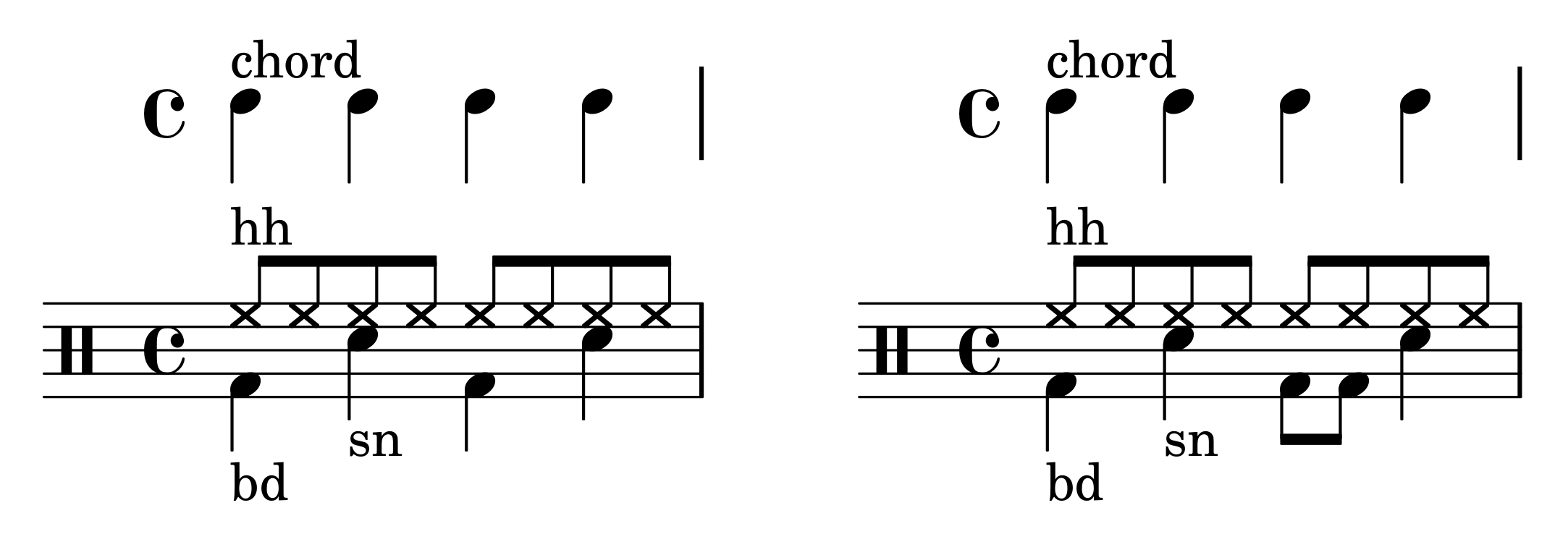
The MIDI files for the mix tracks are created by selecting a random tonic and mode (major or minor diatonic) for the song, and creating random diatonic triad chord sequences in a 4/4 time signature, at a tempo chosen at random between 100 and 200 BPM. Each chord is struck at quarter note intervals for the duration of either one or two measures (chosen at random). All of the chords are in root position, with the root chosen within the MIDI pitch range 48–60. The chords are synthesized by two randomly chosen pitched General MIDI instruments (from the piano, organ, guitar, or orchestral ensemble instrument groups) with a randomly chosen mixing proportion. Additionally, drum tracks are created while using a constant pattern hi-hat, bass drum, and snare (dataset 4 features a different drum pattern than datasets 1–3). Figure 4 displays the patterns. Each of the songs lasts for a variable number of complete measures chosen, such that the song duration is approximately one minute.
In the following subsections, we define the bass patterns for each dataset. Unless specified otherwise, the bass notes are struck at each quarter note, and the bass notes are played in the range of an octave below the root note of the chord. The bass patterns have been chosen, so as to test whether the model can be trained to be sensitive to different musically relevant aspects of the mix. Thus, rather than aiming to provide a set of bass patterns that is representative for actual music (which would be a non-trivial empirical study in itself), we focus on the different aspects of the mix on which such patterns may be conditioned (in particular, harmony, rhythm, and timbre).
5.1.1. Artificial Dataset 1 (A1)
This dataset defines three bass patterns. In pattern 1, the bass plays the first chord degree (the root of the chord). In pattern 2, it plays the third chord degree and, in pattern 3, it plays the fifth chord degree.
5.1.2. Artificial Dataset 2 (A2)
This dataset defines two bass patterns. In pattern 1, the bass plays the first chord degree if the chord is a minor chord, and the fifth chord degree if the chord is a major chord. Conversely, in pattern 2 the bass plays the first chord degree if the chord is a major chord, and the fifth chord degree if the chord is a minor chord.
5.1.3. Artificial Dataset 3 (A3)
Unlike the other datasets, dataset 3 does not use a mix of two randomly chosen instruments to play the chords in the mix track, but instead the instrument is chosen at random at each chord change, and it can be either organ (Drawbar Organ, General MIDI program 17) or guitar (Acoustic Guitar, General MIDI program 25). At each chord change, the probability of switching instrument is 0.5.
This dataset defines two bass patterns. In pattern 1, the bass plays the first chord degree if the chord is played by guitar and the fifth chord degree if the chord is played by organ. Conversely, in pattern 2, the bass plays the first chord degree if the chord is played by organ and the fifth chord degree if the chord is played by guitar.
5.1.4. Artificial Dataset 4 (A4)
Dataset 4 uses a slightly different drum pattern (see Figure 4), in order to be able to define bass patterns that are rhythm specific. Specifically, the third beat of the bar is marked with two eighth note bass drum onsets, instead of a single quarter note.
Dataset 4 defines five bass patterns. In pattern 1, the bass plays the first chord degree on beats one and three (coinciding with the bass drum), and the fifth chord degree on beats two and four (coinciding with the snare drum). Pattern 2 is the converse of pattern 1, with the first chord degree tied to the snare drum and the fifth degree tied to the bass drum. Pattern 3 consists of the following sequence of chord degrees: 1–3–5–3, which is, the first degree on beat one, the third degree on beats two and four, and the fifth degree on beat three. Pattern 4 has a similar “staircase” structure as Pattern 3, but with eighth notes instead of quarter notes: 1–2–3–4–5–4–3–2. Lastly, Pattern 5 consists of a single quarter note on the first chord degree at beat one, and silence throughout the rest of the measure.
5.2. Pop/Rock Dataset (PD)
The Pop/Rock dataset is a proprietary dataset of well-known rock/pop songs of the past decades, including artists, such as Lady Gaga, Coldplay, Stevie Wonder, Lenny Kravitz, Metallica, AC/DC, and Red Hot Chili Peppers. The dataset contains 885 songs from 326 artists, amounting to a total of just over 60 h of music. The average song duration is 245 s with a standard deviation of 74 s. For each song, the stems (guitar, vocals, bass guitar, keyboard, drums) are available as individual audio tracks.
5.3. Training Setup
We train the same architecture with several window sizes, in order to test the effect of temporal context size. The sizes included in the current experiment are 10/10, 20/20, 40/40, 10/20, 10/40, 20/40, 10/640/, 20/640, and 40/640, where a/b denotes a compressed window size of a time steps (see Section 4.3), and an expanded size of b time steps, with a hop time of 0.01 s between timesteps (see Section 4.1). Thus, the compressed window sizes range from 0.1 s to 0.4 s, and the expanded window sizes range from 0.2 s to 6.4 s. All of the models use encoders/decoders consisting of 5 stacked dilated residual blocks (Section 4.4.1), each with 128 feature maps. The dilation of the convolutions is chosen such that the receptive field of the highest block is at least as large as the input both in the time and frequency dimension. The neighborhood size for selecting pairs of instances during training (see Section 4.4.2) is set to 5 s. All of the datasets are split into a training set and validation set according to the proportion 90%/10%. Although we use the latter set for reporting results we do not refer to it as a test set, because it is used for early stopping the training process (see below).
Each model is trained by stochastic optimization of (Equation (9)), while using the Adam method [68] with a batch size of 20 and a learning rate of 0.0001. For the pop/rock dataset, we use on-the-fly random mixing as a form of data augmentation. This means that, for each data instance, the stems of the mix are combined into a mono mix with random mixing coefficients between 0.5 and 1.0, before computing the CQT on the normalized mono mix. After training on a mini epoch of 1000 instances, the validation loss is computed. Training is terminated when the validation loss has not improved for more than 1000 mini epochs for the artificial datasets and 3000 mini epochs for the pop/rock dataset.
6. Results and Discussion
In this section, we report and the discuss the results of training the BassNet architecture separately on each of the datasets (A1–4 and PR), performing various train runs for each dataset, using varying window sizes. We start by comparing the models in terms of the reconstruction loss for the learned descriptors pitch, onset, and level (Section 6.1). After that, we look at the degree to which the models can disentangle the latent bass patterns, as defined in the artificial datasets (Section 6.2). We test the importance of the cross-reconstruction loss for disentangling the bass patterns by way of an ablation study in which we remove the cross-reconstruction terms from the loss function, and instead use the regular reconstruction loss (Section 6.3). Because the models trained on the PR dataset do not allow for this type of groundtruth-based analysis of the latent space, we instead look at the effect of the latent variable on the distribution of predicted bass pitch values relative to the pitch values in the mix (Section 6.4). Lastly, we perform three case studies, in each of which we discuss two distinct bass tracks that were produced by models trained on the pop-rock dataset (Section 6.5).
6.1. Cross-Entropy Loss
Table 1 shows the cross-entropy loss for the pitch, onset, and level predictions of the trained models, computed on the validation data for all if the datasets. The reported values correspond to the CCE (pitch) and BCE (onset and level) terms in Equation (10). The results show—unsurprisingly—that the PR dataset is more challenging than the A1–4 datasets, especially in terms of pitch. Across the board onset is easier to predict than level. This is likely due to the fact that the onset target is sparser.
As for window sizes, the loss results do not reveal an overwhelming winner, even if there appears to be a slight advantage to smaller window sizes. Note that, for onset in the PR dataset, the best results are obtained for the longest window. This is in line with the intuition that the capturing the rhythm of the music requires a larger temporal context.
6.2. Disentanglement of Bass Patterns
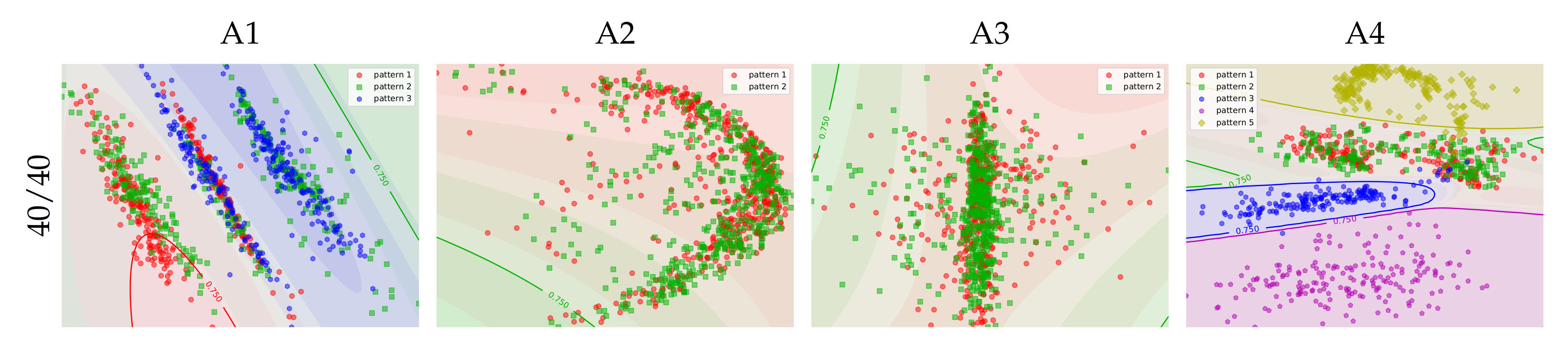
Next, we look at the capability of the models to disentangle the bass patterns that were defined in the artificial datasets. To that end, we plot the latent variable for a subset of the data, coloring each point according to the corresponding bass pattern in the ground truth annotations (Figure 5). More specifically, each point in the plots is the mean of the posterior distribution for a random pair from the validation data, and it is colored according to the bass pattern that was used to produce the bass from the mix when creating the artificial data.
Even if the plots already give a good visual impression of the disentanglement, we can quantify the separation of patterns in the latent space using quadratic discriminant analysis. This analysis consists of estimating a quadratic classifier to predict the pattern c from the latent variable z. It works by defining the pattern-conditional distribution of the latent variable as a multivariate gaussian, and using Bayes rule to infer . For a given instance , the predicted class is defined as the class with the highest conditional probability . The background colors in Figure 5 show how the classifiers partition the latent space into classes. The plots also include the isolines that correspond to for each pattern c. The prediction accuracies of the classifiers serve as a quantitative measure of the disentanglement of the patterns in the learned latent spaces. Table 2 lists the different models and datasets.
The results show that, in most of the cases, but not all, the latent space is organized in order to clearly separate the bass patterns. Models with window size 20/20 and those with expanded window sizes of 40 (i.e., 10/40, 20/40, and 40/40) produce virtually complete disentanglement of bass patterns. Models with longer windows (10/640, 20/640, and 40/640) have difficulty separating the patterns in datasets A2 and A3. In A2, the separation of the bass patterns requires models to successfully recognize the chord type (major vs minor), whereas, in A3, the separation requires sensitivity to instrument timbre in the mix. It is not surprising that, with longer windows, it is more difficult to recognize these aspects of the mix, because the longer windows will almost always span multiple chords, likely with different chord types, and in the case of A3 different instrument timbres. For A1 and A4, the separation of the models with longer windows is clearly visible, but not as clean as the shorter window models. A more surprising result is confusion of patterns in A3 for the 10/10 and 10/20 models, especially since the 20/20 model has no problem finding a clear separation. When comparing the entries of column A3/f0 for models 10/20 and 10/20 in Table 1, the lack of separation of the patterns appears to have a negative impact on the cross-reconstruction loss. A possible explanation for the fact that the short window models fail to capture bass patterns that are conditioned on instrument in A3, is that the windows are too short to capture the temporal dynamics that help to distinguish between guitar and organ.
6.3. Effect of Cross-Reconstruction Loss
The previous section shows that training models with intermediate size windows leads to a disentanglement of bass patterns in the latent space. In this section, we examine to what degree this organization of the latent space is induced by the constraint of temporal stability of latent space trajectories. We do so by way of an ablation study in which we train a model while using the regular reconstruction loss instead of the cross-reconstruction loss. Recall that the original training objective (Equation (9)) involves an instance and a randomly selected nearby neighbor . In that objective, the reconstruction terms , , , and for the instance are computed based on a sample from latent space distribution inferred from its neighbor instance , and vice versa. In this ablation study, we compute the reconstruction terms for based on the latent position inferred from itself. We also omit the Kullback–Leibler divergence between the latent distributions and —the first right-hand term in Equation (9). This yields a training objective that is identical to the test objective given in Equation (10).
With this objective, we train the 40/40 model architecture from the previous experiment, which generally produced clearly disentangled latent representations of the bass patterns. Apart from the training objective, all other training specifics are as in the previous experiment.
Figure 6 and Table 3 show the latent space projection for a subset of the validation set, and the corresponding quadratic classifier prediction accuracies, respectively. Although some clusters form in the latent space, these clusters only occasionally coincide with the bass patterns that underlie the artificial data. Further investigation revealed that the organization sometimes coincides with other factors, such as the absolute pitch of the mix/bass track contents.
This shows that the disentanglement of bass patterns can be largely accounted for by the minimization of the cross-reconstruction loss. The explanation for this is that the cross-reconstruction loss drives the latent space to encode features of the data that remain largely stable over time. Note that the bass patterns in the artificial data only change infrequently, which means that pairs of instances used to compute the cross-reconstruction loss are likely to be generated from the same pattern.
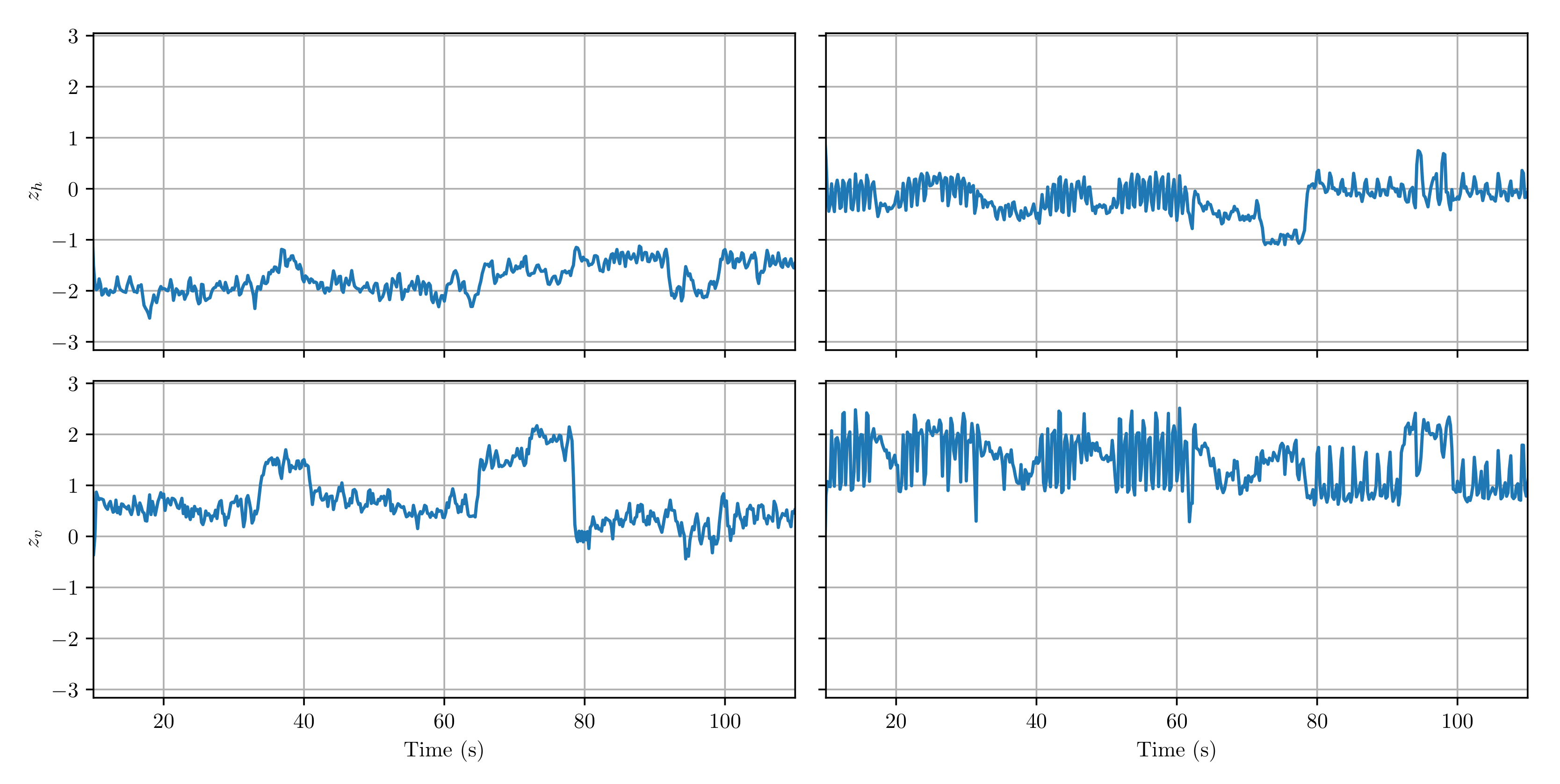
The effect of the cross-reconstruction loss can also be observed when plotting the latent space trajectories over time. Figure 7 shows that the latent space trajectory of the model trained with the regular reconstruction loss (right column) fluctuates more strongly at short time scales, corresponding to changes in absolute pitch. However, because the bass and the guitar play an almost identical riff in this song, encoding the relationship between bass and guitar in terms of relative pitch yields a more stable representation. The disentanglement of the bass patterns in dataset A1 shows that the model (when trained with cross-reconstruction loss) is capable of learning such representations, and indeed using the cross-reconstruction loss (left column) yields a more stable trajectory. Larger jumps in the trajectory (e.g., close to 35 s, 65 s, and 78 s) correspond to transitions between verse and chorus sections of the song.
6.4. Effect of Latent Variable on Relative Pitch Distributions
For the models trained on the PR dataset, an analysis of the latent space as in the previous section is not possible, because of the lack of ground-truth knowledge in terms of bass patterns. Needless to say in actual music such patterns probably exist, but they are much harder to define, and more mixed. This is confirmed by the fact that the data distribution of the latent space (not shown in this paper) is largely unimodal. However, the unimodality of the data distribution does not imply that there is no effect of the latent variable on the output. In this section, we explore how the distribution of values in the predicted bass tracks changes as a function of the latent variable.
Plotting the overall distribution of the predicted bass tracks by itself is not very informative, since averaging distributions for songs with different tonalities would likely blur most of the structure in the distributions of individual songs or song sections. Therefore, we compute the distribution of the predicted bass relative to the of the mix. Such a distribution effectively tells us what pitches the bass plays with respect to predominant pitch of the instruments in the mix. That is, the histogram bin 0 would count the instances where the bass is equal to the mix , whereas the bin −12 (expressed in semitones) would count the instances where the bass is an octave below the mix .
Figure 8 shows the relative distributions for different values of the latent variable z for the validation dataset. The plots have been generated from a model trained on the PR dataset using a window size of 10/80. To highlight the differences between the distributions, we have subtracted from each distribution the relative distribution of the actual bass tracks in the validation dataset. Positive bin values thus indicate a higher occurrence of the relative s than in the data, whereas negative values indicate a lower occurrence. Unsurprisingly, the variation in relative distribution takes place mostly in the negative range (because the bass typically plays below the instruments in the mix). Furthermore, the peaks and valleys at −12 and −24 show that the latent space plays an important role in modulating the frequency of the octaves with respect to each other. Interestingly, the fourths (−19, −31) are also strongly modulated, occasionally with peaks that are as prominent as the octave peaks, for instance, at . This is surprising, since, based on music theory, we would have expected the fifth to play a more important role.
Another notable trend is that the octaves and the fourth are strongly emphasized at the expense of the other diatonic and chromatic intervals in the lower plots, whereas, in the upper left corner, this pattern is reversed. Superficially =, this suggests that the latent space has learned to encode consonance vs dissonance. However, it is important to realize that the distributions are averaged over all songs, and they do not convey and information regarding melody and voice leading.
6.5. Case Studies
In this last part, we present three small case studies. Each case study is a short musical fragment for which two different bass tracks are generated by selecting different positions in the latent space. The latent position remains constant throughout the fragment.
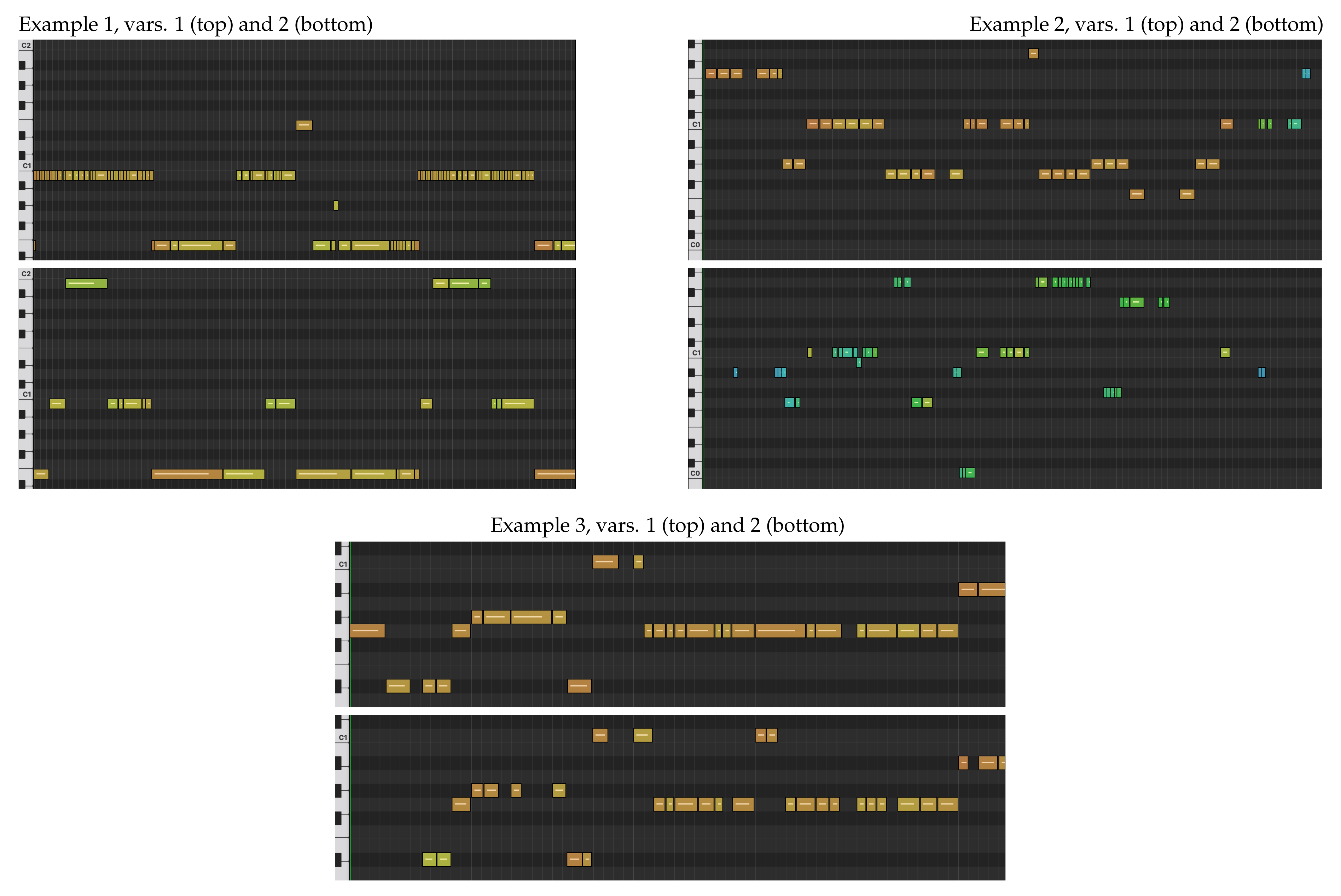
For brevity, we do not display the input tracks here. Instead, we describe the input tracks, and display excerpts of MIDI renderings of the predicted bass tracks (Figure 9). The MIDI renderings were created by peak picking the predicted onset curves, converting the predictions to MIDI notes (including pitch-bend), and setting the MIDI velocity according to the predicted level curves. We recommend listening to the sound examples, available at https://sonycslparis.github.io/bassnet_mdpi_suppl_mat/.
6.5.1. Example 1
The first example is a piano excerpt with strong rubato, but clear onsets. In both examples, BassNet follows the tempo changes and provides realistic harmonies. A notable difference between the variations is that variation 1 tends to rhythmically follow the 16th notes in the higher piano register (but using mostly low pitched notes), whereas variation 2 follows the slower, lower part of the piano (but with higher notes), overall leading to a sparser and quieter result in variation 2.
6.5.2. Example 2
In this example, the source is a polyphonic fragment played by electric bass with non-trivial harmony. For this example, the predicted bass tracks have been transposed one octave upward and quantized to 16th notes. The first variation is created using a latent position that is representative for the training data. The predicted bass line sometimes doubles parts in the source, and it sometimes deviates from them. The output harmony is reasonable and consistent with the input. The rhythm is mostly 8th notes like the source, with occasional 16th notes, which bring groove and variation.
Variation 2 corresponds to a more remote positioning in the latent space. Accordingly, the result is more exotic, and it is reminiscent of improvisation and freestyling or fiddling with the bass. At some point, it remains silent for three seconds, and then goes on again. It is not unlike a human bass player trying something different, succeeding at particular points and failing at others.
6.5.3. Example 3
In this example, the source is a combination of guitar and drums. The drum programming is uncommon, in that it does not feature an alternation of kick and snare. The rhythm of the guitar part is slow and sparse, and the heavy distortion obfuscates the harmony. We believe that providing a bass accompaniment to this example would be not be trivial for a human player. Like in previous examples, the predicted bass is transposed upward one octave and quantized to 16th notes.
Both of the variations are quite similar in terms of pitch, and succeed in following the harmony of the guitar. In terms of rhythm, BassNet produces uncommon grooves, likely in response to the atypical drum track. Varying the latent position, in this case, leads to different grooves.
7. Conclusions and Future Work
In this paper, we have presented BassNet, a deep learning model for conditional generation of bass guitar tracks. Our approach combines several features that we believe jointly allow for interesting music creation use cases. Firstly, rather than creating bass tracks from scratch it allows the user to provide existing musical material. Secondly, the provided audio tracks do not uniquely determine the output. Instead, the user can create a variety of possible bass tracks by varying the two-dimensional learned conditioning signal. Lastly, because the sparse conditioning signal is learned, there is no requirement for annotated data to train the model. This creates the opportunity to train models on specialized user-selected collections of music (for example, their own works, or a specific musical sub-genre).
Using artificial datasets, we have experimentally demonstrated that the model architecture allows for disentangling bass patterns that require a relative pitch representation, and sensitivity to harmony, instrument timbre, and rhythm. Furthermore, we have shown that models trained on a pop/rock dataset learn a latent space that provides musically meaningful control over generated bass tracks in terms of preference for harmonically stable and less harmonically stable pitches. Lastly, we have presented three case studies highlighting the capabilities of the model and possibility of using the latent space as a means of controlling the model output.
We believe an important direction for future work is a better understanding and characterization of the semantics of the latent space learned by the model. At present, the user must explore the latent space by way of trial and error, since there is no indication of which regions of the latent space may yield interesting results for a given input. Inferring and displaying an input-conditional density over the latent space may be a first step in this direction.
A related issue is the focus on user needs. Informal sessions with music producers have provided hints that may not be obvious from a pure research perspective. They prefer richer, more adventurous outputs with occasional errors to a clean output that avoids missteps. This reflects their intended use of BassNet as a tool for providing inspiration, not to produce off-the-shelf musical tracks ready to be included in a mix. A related point is their interest in exploring the limits of the model, for example, by using the model on source material that is very different than the music that the model was trained on. Such issues raise important and interesting methodological challenges.
Author Contributions
Conceptualization: M.G., S.L. and E.D.; Funding acquisition: E.D.; Investigation: M.G.; Methodology: M.G.; Project administration: E.D.; Supervision: M.G.; Validation: M.G., S.L. and E.D.; Visualization: M.G. and S.L.; Writing—original draft: M.G. and S.L.; Writing—review/editing: M.G. and S.L. All authors have read and agreed to the published version of the manuscript.
Funding
This research was funded by Sony Computer Science Laboratories.
Conflicts of Interest
The authors declare no conflict of interest.
References
- Hiller, L.A.; Isaacson, L.M. Experimental Music; Composition with an Electronic Computer; Greenwood Publishing Group Inc.: Westport, CT, USA, 1979. [Google Scholar]
- Lopez de Mantaras, R.; Arcos, J.L. AI and Music: From Composition to Expressive Performance. AI Mag. 2002, 23, 43–57. [Google Scholar]
- Lavrenko, V.; Pickens, J. Polyphonic music modeling with random fields. In Proceedings of the Eleventh ACM International Conference on Multimedia, Berkeley, CA, USA, 2–8 November 2003; Rowe, L.A., Vin, H.M., Plagemann, T., Shenoy, P.J., Smith, J.R., Eds.; ACM: New York, NY, USA, 2003; pp. 120–129. [Google Scholar] [CrossRef]
- Boulanger-Lewandowski, N.; Bengio, Y.; Vincent, P. Modeling Temporal Dependencies in High-Dimensional Sequences: Application to Polyphonic Music Generation and Transcription. In Proceedings of the Twenty-Nine International Conference on Machine Learning (ICML’12), Edinburgh, UK, 26 June–12 July 2012. [Google Scholar]
- Dhariwal, P.; Jun, H.; Payne, C.; Kim, J.W.; Radford, A.; Sutskever, I. Jukebox: A Generative Model for Music. arXiv 2020, arXiv:2005.00341. [Google Scholar]
- Pachet, F.; Roy, P. Imitative Leadsheet Generation with User Constraints. In Proceedings of the ECAI 2014—21st European Conference on Artificial Intelligence, Including Prestigious Applications of Intelligent Systems (PAIS 2014), Prague, Czech Republic, 18–22 August 2014; Schaub, T., Friedrich, G., O’Sullivan, B., Eds.; Frontiers in Artificial Intelligence and Applications. IOS Press: Amsterdam, The Netherlands, 2014; Volume 263, pp. 1077–1078. [Google Scholar] [CrossRef]
- Lattner, S.; Grachten, M.; Widmer, G. Imposing higher-level Structure in Polyphonic Music Generation using Convolutional Restricted Boltzmann Machines and Constraints. J. Creat. Music. Syst. 2018, 3. [Google Scholar] [CrossRef]
- Mehri, S.; Kumar, K.; Gulrajani, I.; Kumar, R.; Jain, S.; Sotelo, J.; Courville, A.C.; Bengio, Y. SampleRNN: An Unconditional End-to-End Neural Audio Generation Model. arXiv 2016, arXiv:1612.07837. [Google Scholar]
- Hadjeres, G.; Pachet, F.; Nielsen, F. DeepBach: A Steerable Model for Bach Chorales Generation. In Proceedings of the 34th International Conference on Machine Learning (ICML 2017), Sydney, NSW, Australia, 6–11 August 2017; Volume 2017, pp. 1362–1371. [Google Scholar]
- Pachet, F. The continuator: Musical interaction with style. J. New Music. Res. 2003, 32, 333–341. [Google Scholar] [CrossRef] [Green Version]
- Vincent, P.; Larochelle, H.; Lajoie, I.; Bengio, Y.; Manzagol, P.A. Stacked denoising autoencoders: Learning useful representations in a deep network with a local denoising criterion. J. Mach. Learn. Res. 2010, 11, 3371–3408. [Google Scholar]
- Makhzani, A.; Shlens, J.; Jaitly, N.; Goodfellow, I.J. Adversarial Autoencoders. arXiv 2015, arXiv:1511.05644. [Google Scholar]
- Kingma, D.P.; Welling, M. Auto-encoding variational bayes. arXiv 2013, arXiv:1312.6114. [Google Scholar]
- Memisevic, R. Gradient-based learning of higher-order image features. In Proceedings of the IEEE International Conference on Computer Vision (ICCV), Barcelona, Spain, 6–13 November 2011; pp. 1591–1598. [Google Scholar]
- Memisevic, R. On multi-view feature learning. In Proceedings of the 29th International Conference on Machine Learning (ICML-12), Edinburgh, UK, 26 June–12 July 2012; Langford, J., Pineau, J., Eds.; Omnipress: New York, NY, USA, 2012; pp. 161–168. [Google Scholar]
- Memisevic, R.; Exarchakis, G. Learning invariant features by harnessing the aperture problem. In Proceedings of the 30th International Conference on Machine Learning, Atlanta, GA, USA, 16–21 June 2013; Volume 28, pp. 100–108. [Google Scholar]
- Memisevic, R.; Hinton, G. Unsupervised learning of image transformations. In Proceedings of the IEEE Conference on Computer Vision and Pattern Recognition, Minneapolis, MN, USA, 17–22 June 2007; pp. 1–8. [Google Scholar]
- Memisevic, R.; Hinton, G.E. Learning to represent spatial transformations with factored higher-order Boltzmann machines. Neural Comput. 2010, 22, 1473–1492. [Google Scholar] [CrossRef]
- Lattner, S.; Grachten, M. High-Level Control of Drum Track Generation Using Learned Patterns of Rhythmic Interaction. In Proceedings of the IEEE Workshop on Applications of Signal Processing to Audio and Acoustics, New Paltz, NY, USA, 20–23 October 2019. [Google Scholar]
- Lattner, S.; Dörfler, M.; Arzt, A. Learning Complex Basis Functions for Invariant Representations of Audio. arXiv 2019, arXiv:1907.05982. [Google Scholar]
- Lattner, S.; Grachten, M.; Widmer, G. Learning Transposition-Invariant Interval Features from Symbolic Music and Audio. In Proceedings of the 19th International Society for Music Information Retrieval Conference, Paris, France, 23–27 September 2018. [Google Scholar]
- Wiskott, L.; Sejnowski, T.J. Slow feature analysis: Unsupervised learning of invariances. Neural Comput. 2002, 14, 715–770. [Google Scholar] [CrossRef]
- Le, Q.V.; Zou, W.Y.; Yeung, S.Y.; Ng, A.Y. Learning hierarchical invariant spatio-temporal features for action recognition with independent subspace analysis. In Proceedings of the 24th IEEE Conference on Computer Vision and Pattern Recognition (CVPR 2011), Colorado Springs, CO, USA, 20–25 June 2011; pp. 3361–3368. [Google Scholar] [CrossRef]
- Olshausen, B.A.; Cadieu, C.; Culpepper, J.; Warland, D.K. Bilinear models of natural images. Electron. Imaging Int. Soc. Opt. Photonics 2007, 6492, 649206. [Google Scholar]
- Eck, D.; Schmidhuber, J. A First Look at Music Composition Using LSTM Recurrent Neural Networks. Ist. Dalle Molle Studi Sull Intell. Artif. 2002, 103, 48. [Google Scholar]
- Liang, F.T.; Gotham, M.; Johnson, M.; Shotton, J. Automatic Stylistic Composition of Bach Chorales with Deep LSTM. In Proceedings of the 18th International Society for Music Information Retrieval Conference, Suzhou, China, 23–27 October 2017; pp. 449–456. [Google Scholar]
- Oore, S.; Simon, I.; Dieleman, S.; Eck, D.; Simonyan, K. This time with feeling: Learning expressive musical performance. Neural Comput. Appl. 2020, 32, 955–967. [Google Scholar] [CrossRef] [Green Version]
- Lyu, Q.; Wu, Z.; Zhu, J.; Meng, H. Modelling High-Dimensional Sequences with LSTM-RTRBM: Application to Polyphonic Music Generation. In Proceedings of the Twenty-Fourth International Joint Conference on Artificial Intelligence, Buenos Aires, Argentina, 25–31 July 2015; pp. 4138–4139. [Google Scholar]
- Cherla, S. Neural Probabilistic Models for Melody Prediction, Sequence Labelling and Classification. Ph.D. Thesis, University of London, London, UK, 2016. [Google Scholar]
- Dong, H.W.; Hsiao, W.Y.; Yang, L.C.; Yang, Y.H. MuseGAN: Multi-track sequential generative adversarial networks for symbolic music generation and accompaniment. In Proceedings of the Thirty-Second AAAI Conference on Artificial Intelligence, New Orleans, LA, USA, 2–7 February 2018. [Google Scholar]
- Yang, L.C.; Chou, S.Y.; Yang, Y.H. MidiNet: A convolutional generative adversarial network for symbolic-domain music generation. arXiv 2017, arXiv:1703.10847. [Google Scholar]
- Liu, H.; Yang, Y. Lead Sheet Generation and Arrangement by Conditional Generative Adversarial Network. In Proceedings of the 17th IEEE International Conference on Machine Learning and Applications (ICMLA), Orlando, FL, USA, 17–20 December 2018; pp. 722–727. [Google Scholar] [CrossRef] [Green Version]
- Huang, C.A.; Vaswani, A.; Uszkoreit, J.; Simon, I.; Hawthorne, C.; Shazeer, N.; Dai, A.M.; Hoffman, M.D.; Dinculescu, M.; Eck, D. Music Transformer: Generating Music with Long-Term Structure. In Proceedings of the International Conference on Learning Representations, New Orleans, LA, USA, 6–9 May 2019. [Google Scholar]
- Payne, C. MuseNet. OpenAI. 2019. Available online: https://openai.com/blog/musenet/ (accessed on 25 April 2019).
- Van den Oord, A.; Dieleman, S.; Zen, H.; Simonyan, K.; Vinyals, O.; Graves, A.; Kalchbrenner, N.; Senior, A.W.; Kavukcuoglu, K. WaveNet: A Generative Model for Raw Audio. In Proceedings of the 9th ISCA Speech Synthesis Workshop, Sunnyvale, CA, USA, 13–15 September 2016. [Google Scholar]
- Engel, J.; Agrawal, K.K.; Chen, S.; Gulrajani, I.; Donahue, C.; Roberts, A. GANSynth: Adversarial Neural Audio Synthesis. In Proceedings of the 7th International Conference on Learning Representations, New Orleans, LA, USA, 6–9 May 2019. [Google Scholar]
- Donahue, C.; McAuley, J.; Puckette, M. Adversarial Audio Synthesis. In Proceedings of the 7th International Conference on Learning Representations, New Orleans, LA, USA, 6–9 May 2019. [Google Scholar]
- Engel, J.; Resnick, C.; Roberts, A.; Dieleman, S.; Norouzi, M.; Eck, D.; Simonyan, K. Neural Audio Synthesis of Musical Notes with WaveNet Autoencoders. In Proceedings of the 34th International Conference on Machine Learning, Sydney, Australia, 6–11 August 2017. [Google Scholar]
- Roberts, A.; Engel, J.; Raffel, C.; Hawthorne, C.; Eck, D. A Hierarchical Latent Vector Model for Learning Long-Term Structure in Music. In Proceedings of the 35th International Conference on Machine Learning, ICML 2018, Stockholmsmässan, Stockholm, Sweden, 10–15 July 2018; pp. 4361–4370. [Google Scholar]
- Simon, I.; Roberts, A.; Raffel, C.; Engel, J.; Hawthorne, C.; Eck, D. Learning a latent space of multitrack measures. arXiv 2018, arXiv:1806.00195. [Google Scholar]
- Aouameur, C.; Esling, P.; Hadjeres, G. Neural Drum Machine: An Interactive System for Real-time Synthesis of Drum Sounds. In Proceedings of the 10th International Conference on Computational Creativity, North Carolina, CA, USA, 17–21 June 2019. [Google Scholar]
- Esling, P.; Masuda, N.; Bardet, A.; Despres, R.; Chemla-Romeu-Santos, A. Universal audio synthesizer control with normalizing flows. arXiv 2019, arXiv:1907.00971. [Google Scholar]
- Nistal, J.; Lattner, S.; Richard, G. DrumGAN: Synthesis of drum sounds with timbral feature conditioning using Generative Adversarial Networks. In Proceedings of the 21st International Society for Music Information Retrieval Conference, Montréal, QC, Canada, 11–15 October 2020. [Google Scholar]
- Ramires, A.; Chandna, P.; Favory, X.; Gómez, E.; Serra, X. Neural Percussive Synthesis Parameterised by High-Level Timbral Features. In Proceedings of the IEEE International Conference on Acoustics, Speech and Signal Processing, Barcelona, Spain, 4–8 May 2020. [Google Scholar]
- Mao, H.H.; Shin, T.; Cottrell, G. DeepJ: Style-specific music generation. In Proceedings of the 2018 IEEE 12th International Conference on Semantic Computing (ICSC), Laguna Hills, CA, USA, 31 January–2 February 2018; pp. 377–382. [Google Scholar]
- Hadjeres, G.; Nielsen, F. Anticipation-RNN: Enforcing unary constraints in sequence generation, with application to interactive music generation. Neural Comput. Appl. 2020, 32, 995–1005. [Google Scholar] [CrossRef] [Green Version]
- Lattner, S.; Grachten, M. Learning Transformations of Musical Material using Gated Autoencoders. In Proceedings of the 2nd Conference on Computer Simulation of Musical Creativity, Milton Keynes, UK, 11–13 September 2017. [Google Scholar]
- Lattner, S.; Grachten, M.; Widmer, G. A predictive model for music based on learned relative pitch representations. In Proceedings of the 19th International Society for Music Information Retrieval Conference, Paris, France, 23–27 September 2018. [Google Scholar]
- Dehghan, A.; Ortiz, E.G.; Villegas, R.; Shah, M. Who do i look like? Determining parent-offspring resemblance via gated autoencoders. In Proceedings of the IEEE Conference on Computer Vision and Pattern Recognition, Columbus, OH, USA, 24–27 June 2014; pp. 1757–1764. [Google Scholar]
- Rimell, L.; Mabona, A.; Bulat, L.; Kiela, D. Learning to Negate Adjectives with Bilinear Models. In Proceedings of the 15th Conference of the European Chapter of the Association for Computational Linguistics, Valencia, Spain, 3–7 April 2017; Volume 2, pp. 71–78. [Google Scholar]
- Mocanu, D.C.; Ammar, H.B.; Lowet, D.; Driessens, K.; Liotta, A.; Weiss, G.; Tuyls, K. Factored four way conditional restricted Boltzmann machines for activity recognition. Pattern Recognit. Lett. 2015, 66, 100–108. [Google Scholar] [CrossRef] [Green Version]
- Droniou, A.; Ivaldi, S.; Sigaud, O. Learning a repertoire of actions with deep neural networks. In Proceedings of the IEEE International Joint Conferences on Development and Learning and Epigenetic Robotics (ICDL-Epirob), Genoa, Italy, 13–16 October 2014; pp. 229–234. [Google Scholar]
- Droniou, A.; Ivaldi, S.; Sigaud, O. Deep unsupervised network for multimodal perception, representation and classification. Robot. Auton. Syst. 2015, 71, 83–98. [Google Scholar] [CrossRef] [Green Version]
- Michalski, V.; Memisevic, R.; Konda, K. Modeling Deep Temporal Dependencies with Recurrent Grammar Cells. In Proceedings of the Advances in Neural Information Processing Systems, Montreal, QC, Canada, 8–13 December 2014; pp. 1925–1933. [Google Scholar]
- Brown, J. Calculation of a constant Q spectral transform. J. Acoust. Soc. Am. 1991, 89, 425–434. [Google Scholar] [CrossRef] [Green Version]
- Cheuk, K.W.; Anderson, H.H.; Agres, K.; Herremans, D. nnAudio: An on-the-fly GPU Audio to Spectrogram Conversion Toolbox Using 1D Convolution Neural Networks. arXiv 2019, arXiv:1912.12055. [Google Scholar] [CrossRef]
- Kim, J.W.; Salamon, J.; Li, P.; Bello, J.P. Crepe: A Convolutional Representation for Pitch Estimation. In Proceedings of the 2018 IEEE International Conference on Acoustics, Speech and Signal Processing (ICASSP), Calgary, AB, Canada, 15–20 April 2018; pp. 161–165. [Google Scholar]
- Böck, S.; Korzeniowski, F.; Schlüter, J.; Krebs, F.; Widmer, G. madmom: A new Python Audio and Music Signal Processing Library. In Proceedings of the 24th ACM International Conference on Multimedia, Amsterdam, The Netherlands, 15–19 October 2016; pp. 1174–1178. [Google Scholar] [CrossRef]
- Schlüter, J.; Böck, S. Musical Onset Detection with Convolutional Neural Networks. In Proceedings of the 6th International Workshop on Machine Learning and Music (MML), Prague, Czech Republic, 23 September 2013. [Google Scholar]
- Brian, M.; Colin, R.; Dawen, L.; Daniel, P.W.E.; Matt, M.; Eric, B.; Oriol, N. librosa: Audio and Music Signal Analysis in Python. In Proceedings of the 14th Python in Science Conference, Austin, TX, USA, 6–12 July 2015; Kathryn, H., James, B., Eds.; pp. 18–24. [Google Scholar]
- Yu, F.; Koltun, V.; Funkhouser, T.A. Dilated Residual Networks. arXiv 2017, arXiv:1705.09914. [Google Scholar]
- He, K.; Zhang, X.; Ren, S.; Sun, J. Deep Residual Learning for Image Recognition. In Proceedings of the IEEE Conference on Computer Vision and Pattern Recognition CVPR, Las Vegas, NV, USA, 26 June–1 July 2016; pp. 770–778. [Google Scholar]
- Chabra, R.; Straub, J.; Sweeney, C.; Newcombe, R.; Fuchs, H. StereoDRNet: Dilated Residual StereoNet. In Proceedings of the 2019 IEEE/CVF Conference on Computer Vision and Pattern Recognition (CVPR), Long Beach, CA, USA, 16–20 June 2019; IEEE Computer Society: Los Alamitos, CA, USA, 2019; pp. 11778–11787. [Google Scholar]
- Goodfellow, I.; Bengio, Y.; Courville, A. Deep Learning; MIT Press: Cambridge, MA, USA, 2016. [Google Scholar]
- Zhang, X.; Tang, X.; Zong, L.; Liu, X.; Mu, J. Deep Multimodal Clustering with Cross Reconstruction. In Advances in Knowledge Discovery and Data Mining; Lauw, H.W., Wong, R.C.W., Ntoulas, A., Lim, E.P., Ng, S.K., Pan, S.J., Eds.; Springer International Publishing: Cham, Switzerland, 2020; pp. 305–317. [Google Scholar]
- Schönfeld, E.; Ebrahimi, S.; Sinha, S.; Darrell, T.; Akata, Z. Cross-Linked Variational Autoencoders for Generalized Zero-Shot Learning. In Proceedings of the International Conference on Learning Representations (ICLR 2019), New Orleans, LA, USA, 6–9 May 2019. [Google Scholar]
- Lattner, S.; Grachten, M. Improving Content-Invariance in Gated Autoencoders for 2D and 3D Object Rotation. arXiv 2017, arXiv:1707.01357. [Google Scholar]
- Kingma, D.P.; Ba, J. Adam: A Method for Stochastic Optimization. In Proceedings of the 3rd International Conference on Learning Representations, San Diego, CA, USA, 7–9 May 2015. [Google Scholar]
Figure 1.
The BassNet model architecture and information flow. The input and target data of the model are shown as grey boxes. Functions are shown as blue rounded boxes. Dark blue boxes depict functions with trainable parameters. White boxes depict computed quantities. The ⊗ sign denotes element-wise multiplication. The green and purple planes denote the parts of the graph that correspond to the encoder functions /, and the decoder function g, respectively. The / boxes represent dilated residual encoders/decoders (Section 4.4.1). The CQT spectrogram computation, feature extraction, and multi-resolution processes are discussed in Section 4.1, Section 4.2, and Section 4.3, respectively.
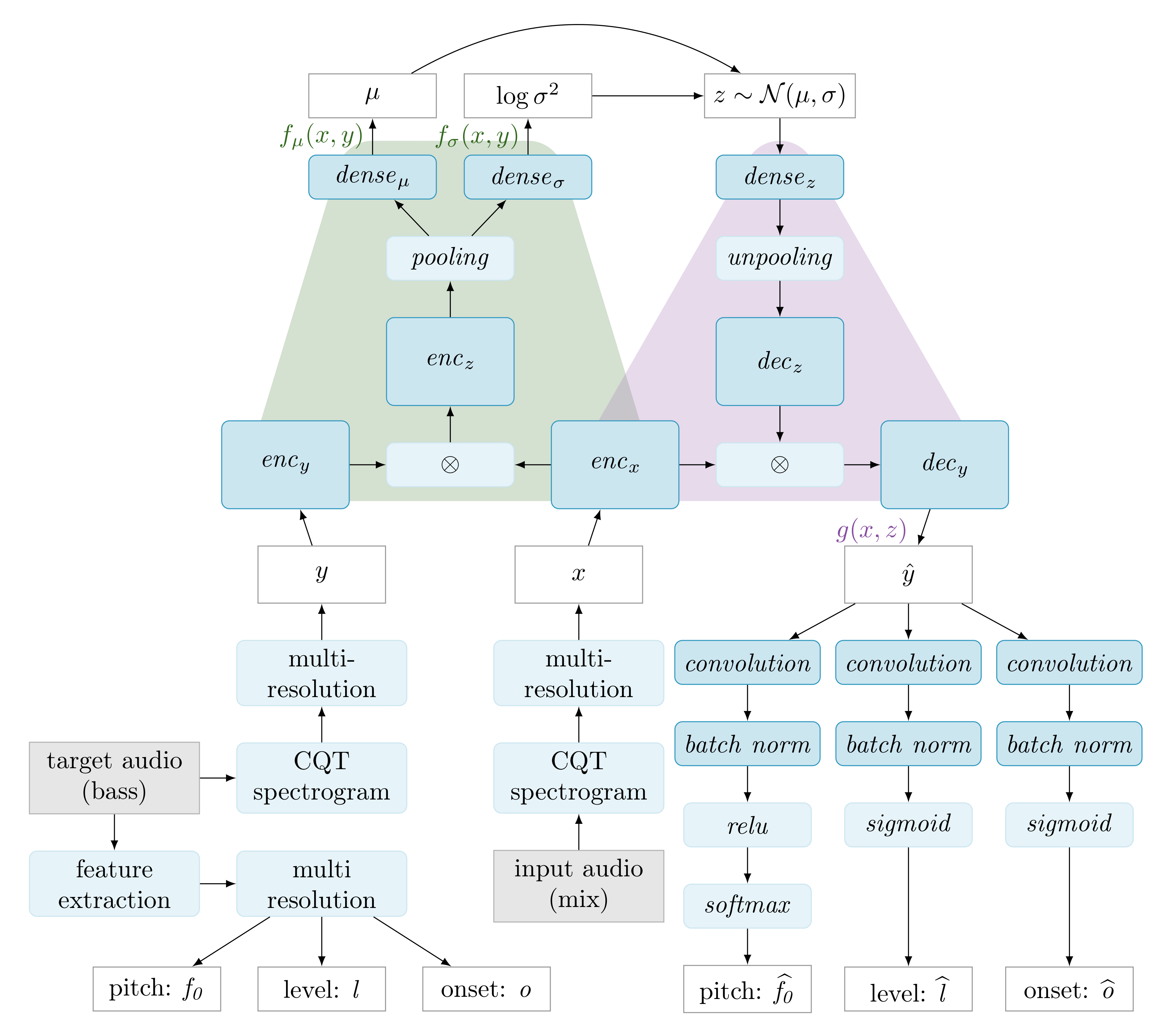
Figure 2.
Schematic illustration of multi-resolution compression and expansion of data windows.
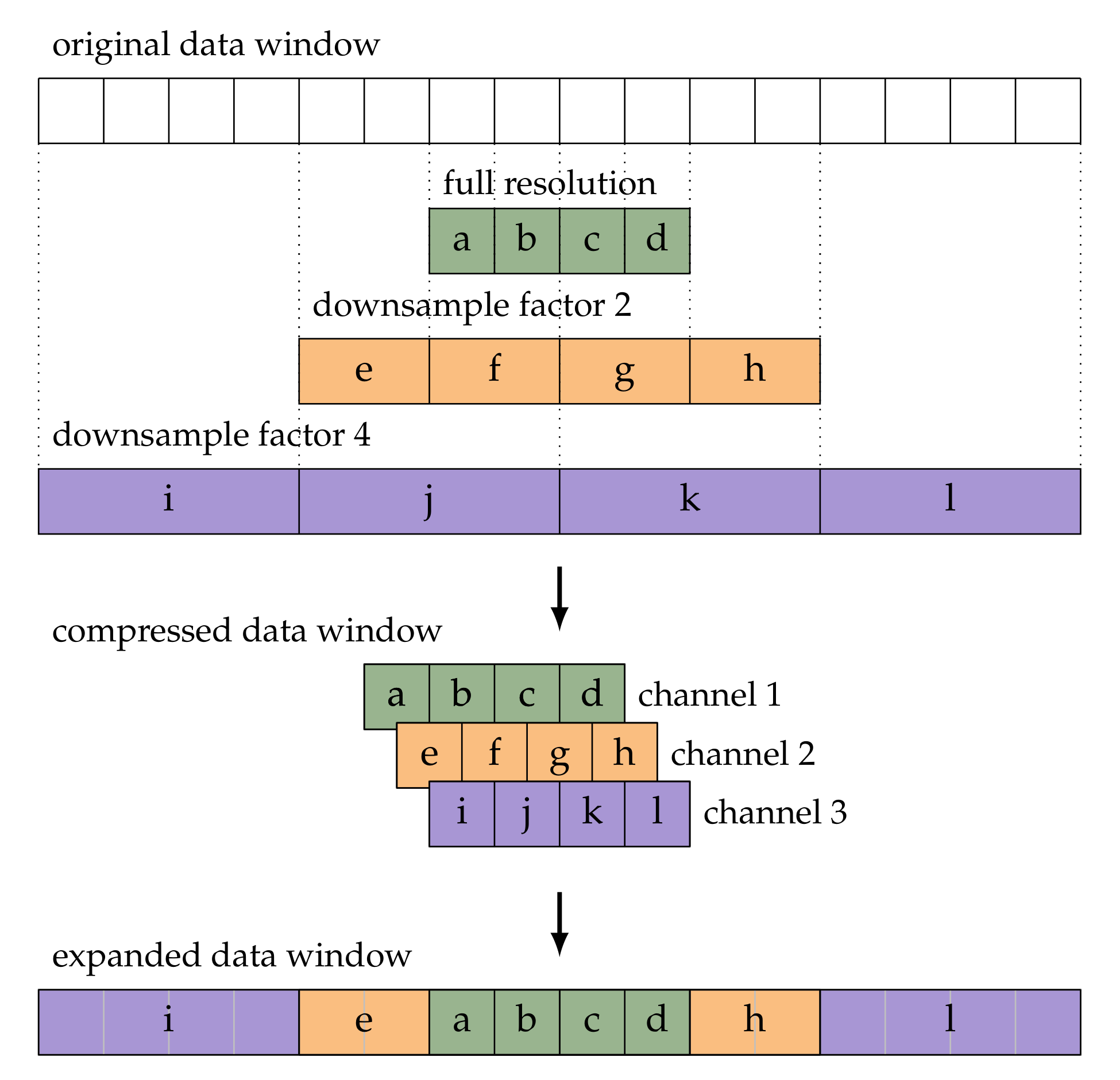
Figure 3.
Dilated residual block.

Figure 4.
Chord and drum patterns for artificial datasets 1–3 (left), and 4 (right).

Figure 5.
Distribution of a subset of the validation data in the latent space. The points are colored according to their corresponding groundtruth bass pattern. The background colors and isolines show the predictions of quadratic classifiers that predict the bass pattern from the latent variable.
Figure 5.
Distribution of a subset of the validation data in the latent space. The points are colored according to their corresponding groundtruth bass pattern. The background colors and isolines show the predictions of quadratic classifiers that predict the bass pattern from the latent variable.
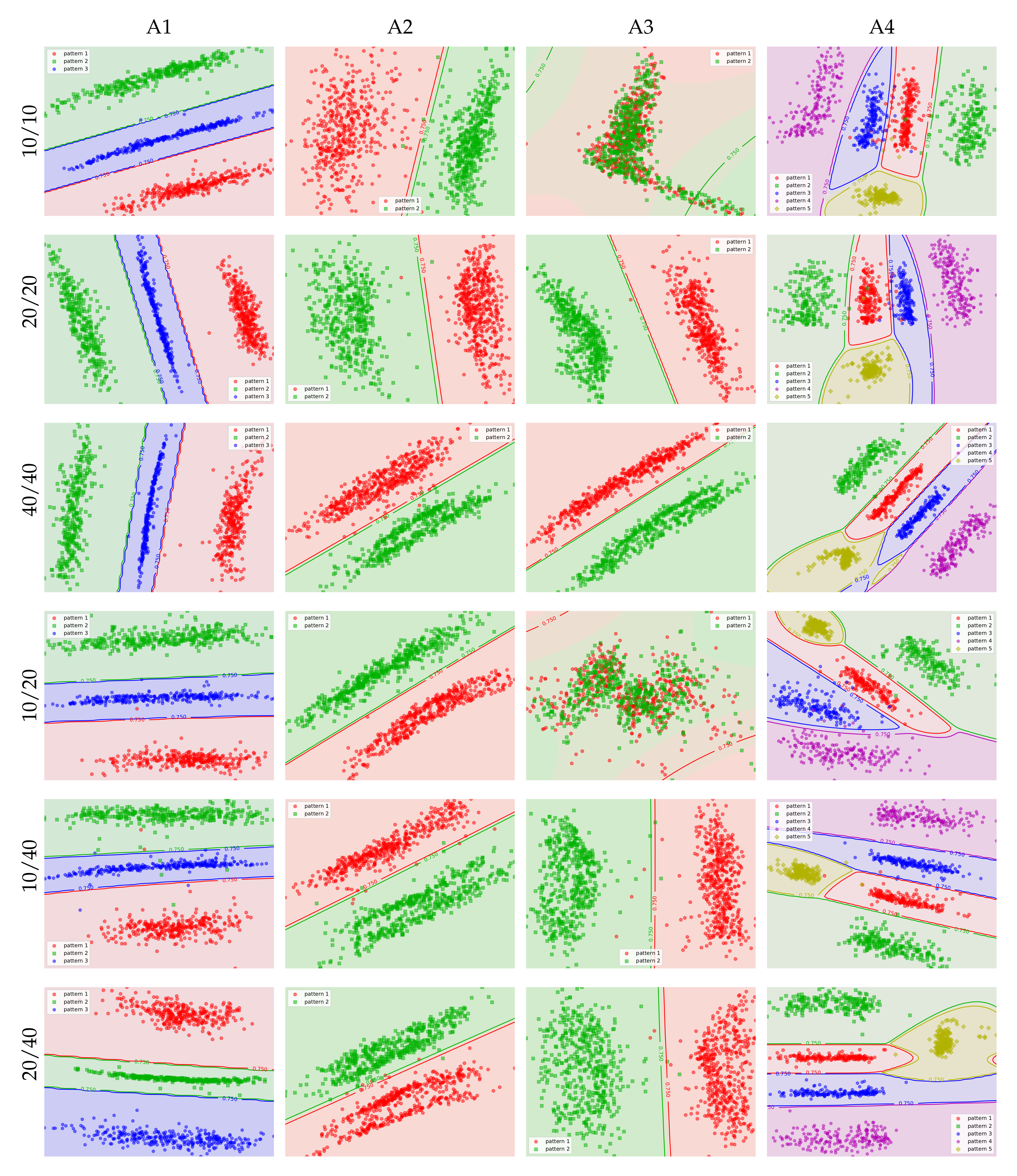
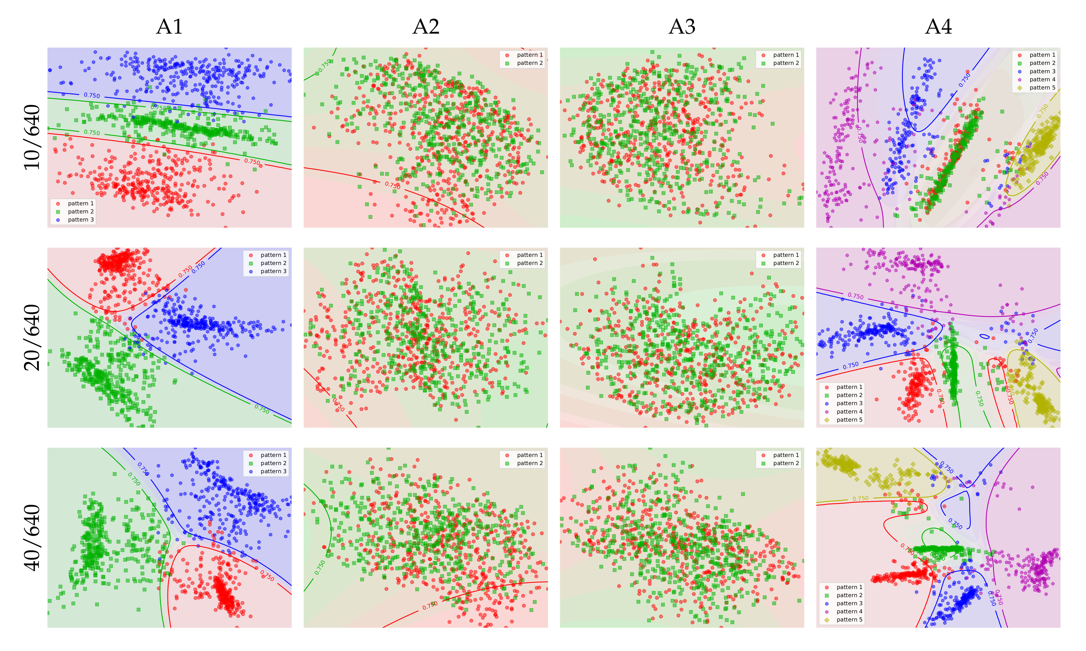
Figure 6.
Organization of the latent space on the 40/40 model trained with regular reconstruction loss instead of cross-reconstruction loss.
Figure 6.
Organization of the latent space on the 40/40 model trained with regular reconstruction loss instead of cross-reconstruction loss.

Figure 7.
Horizonal (top row) and vertical (bottom row) components of the two-dimensional (2D) latent space trajectories for an excerpt of the song Date with the night by Yeah Yeah Yeahs (2003, Polydor). The columns show the trajectories of the models trained with cross-reconstruction loss (left column), and regular reconstruction loss (right column).

Figure 8.
Relative distributions of generated bass tracks with respect to the of the mix, for different values of z. The pitch intervals on the horizontal axis are expressed in semitones. The scale of the vertical axis is arbitrary but identical across plots.
Figure 8.
Relative distributions of generated bass tracks with respect to the of the mix, for different values of z. The pitch intervals on the horizontal axis are expressed in semitones. The scale of the vertical axis is arbitrary but identical across plots.
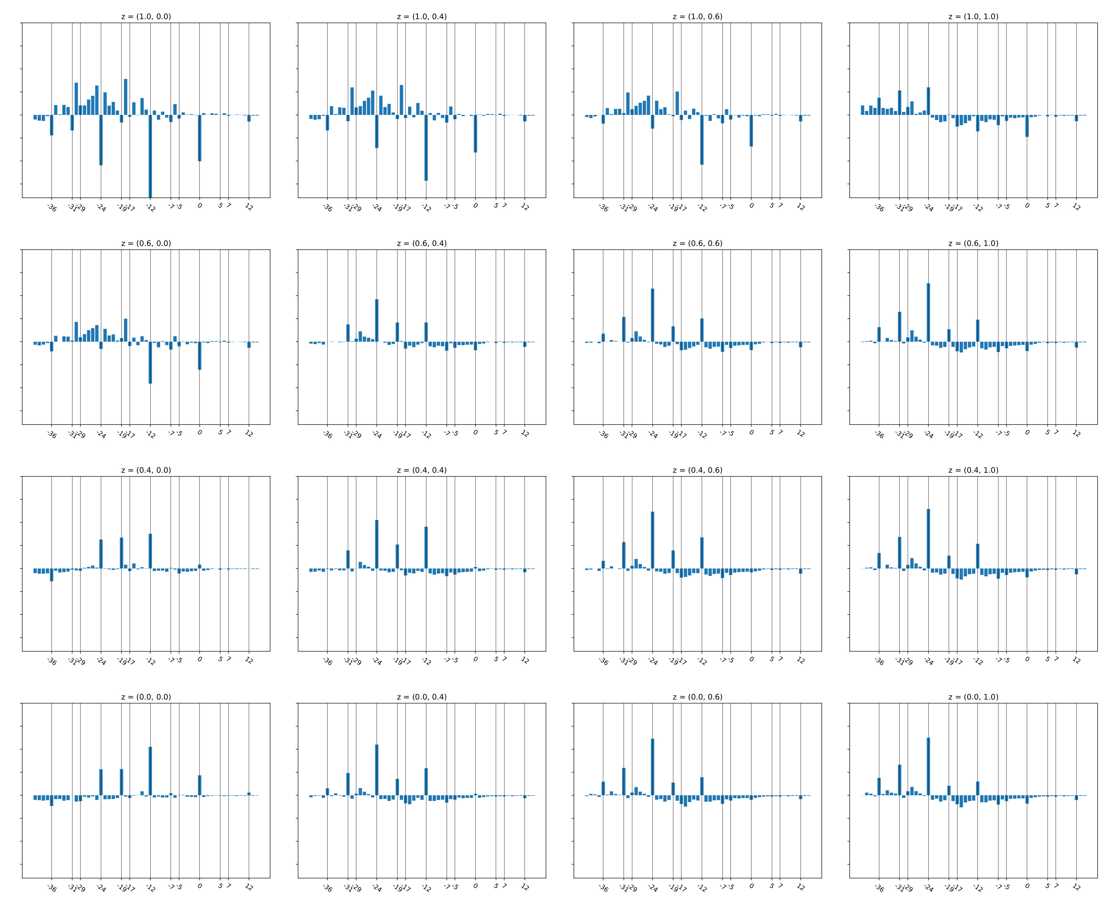
Figure 9.
Pianoroll renderings of generated bass lines. See the text for details.

Table 1.
The cross-entropy loss on validation data of models with varying window sizes, for each of the datasets (A1–4 and PR), and each of the three audio descriptors pitch, level, and onset. The first column specifies the compressed and expanded window sizes of the models.
Table 1.
The cross-entropy loss on validation data of models with varying window sizes, for each of the datasets (A1–4 and PR), and each of the three audio descriptors pitch, level, and onset. The first column specifies the compressed and expanded window sizes of the models.
| A1 | A2 | A3 | A4 | PR | |||||||||||
|---|---|---|---|---|---|---|---|---|---|---|---|---|---|---|---|
| Size | l | o | l | o | l | o | l | o | l | o | |||||
| 10/10 | 0.263 | 0.479 | 0.050 | 0.255 | 0.480 | 0.064 | 0.438 | 0.479 | 0.138 | 0.551 | 0.510 | 0.082 | 1.753 | 0.511 | 0.273 |
| 20/20 | 0.297 | 0.479 | 0.082 | 0.293 | 0.480 | 0.094 | 0.249 | 0.479 | 0.090 | 0.486 | 0.509 | 0.088 | 1.714 | 0.509 | 0.265 |
| 40/40 | 0.312 | 0.480 | 0.075 | 0.284 | 0.480 | 0.068 | 0.268 | 0.479 | 0.086 | 0.487 | 0.504 | 0.094 | 1.707 | 0.515 | 0.263 |
| 10/20 | 0.282 | 0.479 | 0.132 | 0.271 | 0.480 | 0.146 | 0.383 | 0.479 | 0.090 | 0.557 | 0.513 | 0.086 | 1.718 | 0.509 | 0.266 |
| 10/40 | 0.308 | 0.479 | 0.087 | 0.294 | 0.482 | 0.192 | 0.295 | 0.479 | 0.115 | 0.419 | 0.498 | 0.086 | 1.767 | 0.515 | 0.351 |
| 20/40 | 0.288 | 0.479 | 0.080 | 0.265 | 0.480 | 0.123 | 0.279 | 0.479 | 0.086 | 0.421 | 0.497 | 0.081 | 1.725 | 0.510 | 0.276 |
| 10/640 | 0.676 | 0.480 | 0.168 | 0.621 | 0.480 | 0.142 | 0.634 | 0.481 | 0.215 | 0.986 | 0.537 | 0.169 | 1.719 | 0.511 | 0.268 |
| 20/640 | 0.632 | 0.480 | 0.141 | 0.661 | 0.480 | 0.160 | 0.542 | 0.479 | 0.151 | 0.738 | 0.533 | 0.118 | 1.729 | 0.515 | 0.269 |
| 40/640 | 0.618 | 0.480 | 0.132 | 0.655 | 0.480 | 0.129 | 0.644 | 0.518 | 0.313 | 0.732 | 0.523 | 0.112 | 1.724 | 0.513 | 0.268 |
Table 2.
Predictive accuracy of the quadratic classifiers.
| Size | A1 | A2 | A3 | A4 |
|---|---|---|---|---|
| 10/10 | 0.999 | 0.996 | 0.515 | 0.982 |
| 20/20 | 1.000 | 0.998 | 0.999 | 0.985 |
| 40/40 | 1.000 | 0.996 | 1.000 | 0.999 |
| 10/20 | 0.999 | 1.000 | 0.540 | 0.988 |
| 10/40 | 0.991 | 0.991 | 0.995 | 0.993 |
| 20/40 | 1.000 | 0.994 | 0.996 | 0.999 |
| 10/640 | 0.965 | 0.551 | 0.536 | 0.729 |
| 20/640 | 0.975 | 0.560 | 0.526 | 0.912 |
| 40/640 | 0.965 | 0.599 | 0.554 | 0.919 |
Table 3.
Predictive accuracy of the quadratic classifiers for models trained with regular reconstruction loss instead of cross-reconstruction loss.
Table 3.
Predictive accuracy of the quadratic classifiers for models trained with regular reconstruction loss instead of cross-reconstruction loss.
| Size | A1 | A2 | A3 | A4 |
|---|---|---|---|---|
| 40/40 | 0.445 | 0.564 | 0.530 | 0.801 |
© 2020 by the authors. Licensee MDPI, Basel, Switzerland. This article is an open access article distributed under the terms and conditions of the Creative Commons Attribution (CC BY) license (http://creativecommons.org/licenses/by/4.0/).
Share and Cite
MDPI and ACS Style
Grachten, M.; Lattner, S.; Deruty, E. BassNet: A Variational Gated Autoencoder for Conditional Generation of Bass Guitar Tracks with Learned Interactive Control. Appl. Sci. 2020, 10, 6627. https://doi.org/10.3390/app10186627
AMA Style
Grachten M, Lattner S, Deruty E. BassNet: A Variational Gated Autoencoder for Conditional Generation of Bass Guitar Tracks with Learned Interactive Control. Applied Sciences. 2020; 10(18):6627. https://doi.org/10.3390/app10186627
Chicago/Turabian StyleGrachten, Maarten, Stefan Lattner, and Emmanuel Deruty. 2020. "BassNet: A Variational Gated Autoencoder for Conditional Generation of Bass Guitar Tracks with Learned Interactive Control" Applied Sciences 10, no. 18: 6627. https://doi.org/10.3390/app10186627
Note that from the first issue of 2016, this journal uses article numbers instead of page numbers. See further details here.