Experimental Study of Electrical Properties of Pharmaceutical Materials by Electrical Impedance Spectroscopy

 , ,
, ,  and
and 
Abstract
1. Introduction
2. Materials and Methods
2.1. Frequency Response Measurement Methods
- (1)
- The frequency measurement range should be suitable for capturing the frequency response of the process accurately over a high-frequency range (Figure 1).
- (2)
- The measurement method should provide an accurate impedance measurement over the entire frequency measurement range.
- (3)
- The method should require minimal calibration procedure.
- (4)
- The measurement method must be suitable for measuring the properties of the test bulk material.
2.2. Sensing Electrode Array
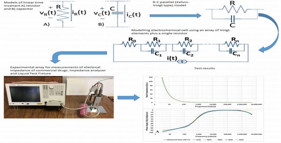
2.3. Basic Electrochemical Electrical Equivalent Circuit (EEC) Models
2.4. Representation of Basic Kelvin–Voigt Electrochemical Cell Models
2.5. State-Space Modelling in the Frequency Domain
2.6. Estimation of Equivalent R-C Network Model
2.7. Measurement Setup
- (a)
- Electrode size: 38 ± 0.5 (mm) (circular geometry).
- (b)
- Casing dimensions: 85 height × 85 width × 37 depth (mm).
- (c)
- Materials (electrodes, spacers, liquid inlet and outlet): nickel-plated cobal (Fe 54%, Co 17%, Ni 29%).
- (d)
- Insulator: ceramic insulator (alumina Al2O3).
- (e)
- O-ring: Viton (Fluoro rubber).
- (f)
- Insulator soldering: silver-copper and gold copper.
2.8. Determination of the Order Model
3. Results
Identification of the Model Components
4. Conclusions
Author Contributions
Funding
Conflicts of Interest
References
- Siddiqui, M.R.; AlOthman, Z.A.; Rahman, N. Analytical techniques in pharmaceutical analysis: A review. Arab. J. Chem. 2017, 10, 1409–1421. [Google Scholar] [CrossRef]
- Randviir, E.P.; Banks, C.E. Electrochemical impedance spectroscopy: An overview of bioanalytical applications. Anal. Methods UK 2013, 5, 1098–1149. [Google Scholar] [CrossRef]
- Grossi, M.; Riccò, B. Electrical impedance spectroscopy (EIS) for biological analysis and food characterization: A review. J. Sens. Sens. Syst. 2017, 6, 303–325. [Google Scholar] [CrossRef]
- Ragoisha, G.A. Challenge for electrochemical impedance spectroscopy in the dynamic world. J. Solid State Electr. 2020, 24, 2171–2172. [Google Scholar] [CrossRef]
- Rimpiläinen, V.; Kuosmanen, M.; Ketolainen, J.; Järvinen, K.; Vauhkonen, M.; Heikkinen, L.M. Electrical impedance tomography for three-dimensional drug release monitoring. Eur. J. Pharm. Sci. 2010, 41, 407–413. [Google Scholar] [CrossRef]
- Gabriel, C.; Gabriel, S.; Corthout, E. The dielectric properties of biological tissues: I. Literature survey. Phys. Med. Biol. 1996, 41, 2231–2249. [Google Scholar] [CrossRef]
- Gabriel, S.; Lau, R.W.; Gabriel, C. The dielectric properties of biological tissues: II. Measurements in the frequency range 10 Hz to 20 GHz. Phys. Med. Biol. 1996, 41, 2251–2269. [Google Scholar] [CrossRef]
- Gabriel, S.; Lau, R.W.; Gabriel, C. The dielectric properties of biological tissues: III. Parametric models for the dielectric spectrum of tissues. Phys. Med. Biol. 1996, 41, 2271–2293. [Google Scholar] [CrossRef]
- Clemente, F.; Arpaia, P.; Manna, C. Characterization of human skin impedance after electrical treatment for transdermal drug delivery. Measurement 2013, 46, 3494–3501. [Google Scholar] [CrossRef]
- Grossi, M.; Parolin, C.; Vitali, B.; Riccò, B. Electrical Impedance Spectroscopy (EIS) Characterization of saline solutions with a low-cost portable measurement system. Eng. Sci. Technol. 2019, 22, 102–108. [Google Scholar] [CrossRef]
- Keysight Technologies. A Guide to Measurement Technology and Techniques, 6th ed.; Impedance Measurement Handbook. Document 5950–3000; Available online: https://www.keysight.com/us/en/assets/7018-06840/application-notes/5950-3000.pdf (accessed on 10 July 2020).
- Newman, J. Resistance for flow of current to a disk. J. Electrochem. Soc. 1966, 113, 501–502. [Google Scholar] [CrossRef]
- Newman, J. Frequency dispersion in capacity measurements at a disk electrode. J. Electrochem. Soc. 1970, 117, 198–203. [Google Scholar] [CrossRef]
- Davis, K.; Dizon, A.; Alexander, C.L.; Orazem, M.E. Influence of geometry-induced frequency dispersion on the impedance of rectangular electrodes. Electrochim. Acta 2018, 283, 1820–1828. [Google Scholar] [CrossRef]
- Gharbi, O.; Dizon, A.; Orazem, M.E.; Tran, M.T.T.; Tribollet, B.; Vivier, V. From frequency dispersion to Ohmic impedance: A new insight on the high-frequency impedance analysis of electrochemical systems. Electrochim. Acta 2019, 320, 134609. [Google Scholar] [CrossRef]
- Levent, A.; Yardım, Y.; Şentürk, Z. Electrochemical performance of boron-doped diamond electrode in surfactant-containing media for ambroxol determination. Sens. Actuators B-Chem. 2014, 203, 517–526. [Google Scholar] [CrossRef]
- Yari, A.; Shams, A. Silver-filled MWCNT nanocomposite as a sensing element for voltammetric determination of sulfamethoxazole. Anal. Chim. Acta 2018, 1039, 51–58. [Google Scholar] [CrossRef]
- Sgobbi, F.L.; Razzino, A.C.; Machado, A.S. A disposable electrochemical sensor for simultaneous detection of sulfamethoxazole and trimethoprim antibiotics in urine based on multiwalled nanotubes decorated with Prussian blue nanocubes modified screen-printed electrode. Electrochim. Acta 2016, 191, 1010–1017. [Google Scholar] [CrossRef]
- Chen, C.; Chen, C.Y.; Hong, T.Y.; Lee, W.T.; Huang, F.J. Facile fabrication of ascorbic acid reduced graphene oxide-modified electrodes toward electroanalytical determination of sulfamethoxazole in aqueous environments. Chem. Eng. J. 2018, 352, 188–197. [Google Scholar] [CrossRef]
- 20. Gamry Instruments, Basics of Electrochemical Impedance (Application Note). Available online: https://www.gamry.com/application-notes/EIS/basics-of-electrochemical-impedance-spectroscopy/ (accessed on 10 July 2020).
- Sindhuja, M.; Kumar, N.S.; Sudha, V.; Harinipriya, S. Equivalent circuit modeling of microbial fuel cells using impedance spectroscopy. J. Energy Storage 2016, 7, 136–146. [Google Scholar] [CrossRef]
- Ahmad, Z.; Mishra, A.; Abdulrahim, S.M.; Touati, F. Electrical equivalent circuit (EEC) based impedance spectroscopy analysis of HTM free perovskite solar cells. J. Electroanal. Chem. 2020, 871, 114294. [Google Scholar] [CrossRef]
- Liao, H.; Watson, W.; Dizon, A.; Tribollet, B.; Vivier, V.; Orazem, M.E. Physical properties obtained from measurement model analysis of impedance measurements. Electrochim. Acta 2020, 354, 136747. [Google Scholar] [CrossRef]
- Agarwal, P.; Orazem, M.E.; Garcia-Rubio, L.H. Measurement models for electrochemical impedance spectroscopy I. Demonstration of Applicability. J. Electrochem. Soc. 1992, 139, 1917–1927. [Google Scholar] [CrossRef]
- Pavel, C.; Przemyslaw, D. Electrochemical Impedance Spectroscopy as a tool for electrochemical rate constant estimation. J. Vis. Exp. 2018, 140, 56611. [Google Scholar]
- Ramos-Barrado, J.R.; Montenegro, G.P.; Cambon, C.C. A generalized Warburg Impedance for a nonvanishing relaxation process. J. Chem. Phys. 1996, 105, 2813. [Google Scholar] [CrossRef]
- Huang, J. Diffusion impedance of electroactive materials, electrolytic solutions and porous electrodes: Warburg impedance and beyond. Electrochim. Acta 2018, 281, 170–188. [Google Scholar] [CrossRef]
- Saatci, E.; Saatci, E.; Akan, A. Analysis of linear lung models based on state-space models. Comput. Methods Prog. Biomed. 2020, 183, 105094. [Google Scholar] [CrossRef]
- Chen, C.W.; Juang, J.N.; Lee, G. Frequency Domain State-Space System Identification. In Proceedings of the 1993 American Control Conference, American Automatic Control Council, San Francisco, CA, USA, 2–4 June 1993; pp. 3057–3061. [Google Scholar] [CrossRef]
- Keysight Technologies. Keysight 16452A Liquid Test Fixture, Operation and Service Manual. Document 16452–90000. Available online: https://www.keysight.com (accessed on 10 July 2020).
- Chuealee, R.; Aramwit, P.; Srichana, T. Characteristics of cholesteryl cetyl carbonate liquid crystals as drug delivery systems. In Proceedings of the 2nd IEEE International Conference on Nano/Micro Engineered and Molecular Systems, Bangkok, Thailand, 16–19 January 2007; pp. 1098–1103. [Google Scholar]
- Guascito, M.R.; Alfinito, E.; Cataldo, R.; Giotta, L. Tips for a (simple) Interpretation of the impedance response of an electrochemical cell. IEEE Sens. J. 2019, 19, 11318–11322. [Google Scholar] [CrossRef]
- Akaike, H. A new look at the statistical model identification. IEEE T. Automat. Control 1974, 19, 716–723. [Google Scholar] [CrossRef]
- Valsa, J.; Dvořák, P.; Friedl, M. Network model of the CPE. Radioengineering 2011, 20, 619–626. [Google Scholar]
- Schwake, A.; Geuking, H.; Cammann, K. Application of a new graphical fitting approach for data analysis in electrochemical impedance spectroscopy. Electroanalysis 1999, 10, 1026–1029. [Google Scholar] [CrossRef]
- Huang, J.; Li, Z.; Liaw, B.Y.; Zhang, J. Graphical analysis of electrochemical impedance spectroscopy data in Bode and Nyquist representations. J. Power Sources 2016, 309, 82–98. [Google Scholar] [CrossRef]
- Ragoisha, G.A.; Bondarenko, A.S. Potentiodynamic electrochemical impedance spectroscopy. Electrochim. Acta 2005, 50, 1553–1563. [Google Scholar] [CrossRef]
- Bodarenko, A.S.; Ragoisha, G.A. Inverse problem in potentiodynamic electrochemical impedance spectroscopy. In Chapter 7 in Progress in Chemometrics Research; Pomerantsev, A.L., Ed.; Nova Science: New York, NY, USA, 2005; pp. 89–102. [Google Scholar]
- Wang, J. Real-time electrochemical monitoring: Toward green analytical chemistry. Acc. Chem. Res. 2002, 35, 811–816. [Google Scholar] [CrossRef] [PubMed]
- Mishra, R.K.; Nunes, G.S.; Souto, L.; Marty, J.L. Screen printed technology—An application towards biosensor development. In Encyclopedia of Interfacial Chemistry; Klaus, W., Ed.; Elsevier: Amsterdam, The Netherlands, 2018; pp. 487–498. [Google Scholar]
- Mora, L.; Chumbimuni-Torres, K.Y.; Clawson, C.; Hernandez, L.; Zhang, L.; Wang, J. Real-time electrochemical monitoring of drug release from therapeutic nanoparticles. J. Control. Release 2009, 140, 69–73. [Google Scholar] [CrossRef] [PubMed]
- Alizadeh, N.; Shamaeli, E.; Fazili, M. Online spectroscopic monitoring of drug release kinetics from nanostructured dual-stimuli-responsive conducting polymer. Pharm. Res. 2017, 34, 113–120. [Google Scholar] [CrossRef]
- Lochner, T.; Perchthaler, M.; Binder, J.T.; Sabawa, J.P.; Dao, T.A.; Bandarenka, A.S. Real-time impedance analysis for the on-road monitoring of automotive fuel cells. Chem. Eur. Soc. Publ. 2020, 7, 2784–2791. [Google Scholar]


| Measurement Method | Advantages | Disadvantages | Applicable Frequency Range | Applications |
|---|---|---|---|---|
| Bridge | High accuracy (0.1% typically) Wide frequency range coverage by using different types of bridges Low Cost | Needs to be manually balanced Narrow frequency coverage with a single instrument | DC to 300 MHz | Standard Lab |
| Resonant method | Good Q accuracy up to high Q | Needs to be tuned to resonance Low impedance measurement accuracy | 10 kHz to 70 MHz | High-Q device measurement |
| Current–voltage (I–V) | Grounded device measurement Suitable to probe-type test needs | Operating frequency range is limited by transformer used in probe | 10 kHz to 100 MHz | Grounded device measurement |
| RF I–V | High accuracy (1% typ.) and wide impedance range at high frequencies | Operating frequency range is limited by transformer used in test head | 1 MHz to 3 GHz | RF component measurement |
| Network analysis | Wide frequency coverage from LF to RF Good accuracy when the unknown impedance is close to characteristic impedance | Recalibration required when the measurement frequency is changed Narrow impedance measurement range | 5 Hz and above | RF component measurement |
| Auto-balancing bridge | Wide frequency coverage from LF to HF High accuracy over a wide impedance measurement range Grounded device measurement | High frequency range not available | 20 Hz to 120 MHz | Generic component measurement Grounded device measurement |
| Trimethoprim/Sulfamethoxazole | Suspension |
| Oxolvan (Ambroxol) | Suspension |
| Magnil (Metamizole Sodium) | Syrup |
| Ranitidine | Injectable solution |
| Transfer function | Poles | 2 | 3 | 3 | 4 | 4 |
| Zeroes | 2 | 2 | 3 | 3 | 4 | |
| Electrical model | Number of model parameters | 5 | 6 | 7 | 8 | 9 |
| Number of resistances | 3 | 3 | 4 | 4 | 5 | |
| Number of capacitors | 2 | 3 | 3 | 4 | 4 | |
| Akaike information Criterion | % Fit | 94.83 | 98.02 | 94.862 | 97.776 | 97.646 |
| Mean Squared Error (MSE) | 1.016 | 0.15 | 1.005 | 0.1883 | 0.211 | |
| Final Prediction Error (FPE) | 1.042 | 0.1546 | 1.041 | 0.196 | 0.2206 | |
| Number of samples | 201 | 201 | 201 | 201 | 201 | |
| AIC | 1157 | 390.2 | 1157 | 485.6 | 533 | |
| AICc | 1157 | 390.5 | 1157 | 486 | 534 | |
| Controllability/Observability analysis | Rank observability | 2 | 3 | 3 | 1 | 1 |
| Unobservable states | 0 | 0 | 0 | 3 | 3 | |
| Rank controllability | 2 | 1 | 3 | 1 | 1 | |
| Uncontrollable states | 0 | 2 | 0 | 3 | 3 | |
| max log (Hankel SV) | 7.61 | 16.52 | * | * | * |
| Transfer Function | Poles | 2 | 3 | 3 | 4 | 4 |
| Zeroes | 2 | 2 | 3 | 3 | 4 | |
| Electrical Model | Number of Model Parameters | 5 | 6 | 7 | 8 | 9 |
| Number of resistances | 3 | 3 | 4 | 4 | 5 | |
| Number of Capacitors | 2 | 3 | 3 | 4 | 4 | |
| Akaike Information Criterion | % Fit | 94.4 | 98.6 | 98 | 98.8 | 97.6 |
| Mean Squared Error (MSE) | 1.569 | 0.094 | 0.2026 | 0.0776 | 0.297 | |
| Final Prediction Error (FPE) | 1.608 | 0.0968 | 0.2098 | 0.0808 | 0.3106 | |
| Number of Samples | 201 | 201 | 201 | 201 | 201 | |
| AIC | 1332 | 202.3 | 513.1 | 129.5 | 670.8 | |
| AICc | 1332 | 202.5 | 513.4 | 129.8 | 671.3 | |
| Controllability/Observability Analysis | Rank Observability | 2 | 3 | 3 | 1 | 4 |
| Unobservable States | 0 | 0 | 0 | 3 | 0 | |
| Rank Controllability | 2 | 1 | 3 | 1 | 4 | |
| Uncontrollable States | 0 | 2 | 0 | 3 | 0 | |
| max log (Hankel SV) | 6.676 | 16.14 | * | * | * |
| Transfer Function | Poles | 2 | 3 | 3 | 4 | 4 |
| Zeroes | 2 | 2 | 3 | 3 | 4 | |
| Electrical Model | Number of Model Parameters | 5 | 6 | 7 | 8 | 9 |
| Number of resistances | 3 | 3 | 4 | 4 | 5 | |
| Number of Capacitors | 2 | 3 | 3 | 4 | 4 | |
| Akaike Information Criterion | % Fit | 93.11 | 97.69 | 97.37 | 97.73 | 97.76 |
| Mean Squared Error (MSE) | 10.69 | 1.199 | 1.551 | 1.16 | 1.123 | |
| Final Prediction Error (FPE) | 10.96 | 1.235 | 1.606 | 1.207 | 1.175 | |
| Number of Samples | 201 | 201 | 201 | 201 | 201 | |
| AIC | 2103.427 | 1225.763 | 1331.341 | 1216.477 | 1205.560 | |
| AICc | 2103.578 | 1225.975 | 1331.626 | 1216.843 | 1206.020 | |
| Controllability/Observability Analysis | Rank Observability | 2 | 3 | 3 | 3 | 1 |
| Unobservable States | 0 | 0 | 0 | 1 | 3 | |
| Rank Controllability | 2 | 1 | 1 | 2 | 1 | |
| Uncontrollable States | 0 | 2 | 2 | 2 | 3 | |
| max log (Hankel SV) | 5.710 | 16.756 | 6.431 | 16.765 | 6.878 |
| Transfer Function | Poles | 2 | 3 | 3 | 4 | 4 |
| Zeroes | 2 | 2 | 3 | 3 | 4 | |
| Electrical Model | Number of Model Parameters | 5 | 6 | 7 | 8 | 9 |
| Number of resistances | 3 | 3 | 4 | 4 | 5 | |
| Number of Capacitors | 2 | 3 | 3 | 4 | 4 | |
| Akaike Information Criterion | % Fit | 90.15 | 90.15 | 97.09 | 99.65 | 99.65 |
| Mean Squared Error (MSE) | 5.275 | 5.275 | 0.04882 | 0.006531 | 0.006531 | |
| Final Prediction Error (FPE) | 5.407 | 5.435 | 0.05087 | 0.006793 | 0.00683 | |
| Number of Samples | 201 | 201 | 201 | 201 | 201 | |
| AIC | 1819 | 1821 | −48.12 | −865.7 | −863.7 | |
| AICc | 1819 | 1821 | −47.78 | −865.4 | −863.3 | |
| Controllability/Observability Analysis | Rank Observability | 2 | 3 | 3 | 1 | 1 |
| Unobservable States | 0 | 0 | 0 | 3 | 3 | |
| Rank Controllability | 2 | 1 | 3 | 1 | 1 | |
| Uncontrollable States | 0 | 2 | 0 | 3 | 3 | |
| max log (Hankel SV) | * | * | * | 15.47 | 7.91 |
| Electrical Component | Ranitidine | Metamizole | Ambroxol | Trimethoprim Sulfamethoxazole |
|---|---|---|---|---|
| % Fit = 90.15 | % Fit = 94.83 | % Fit = 94.38 | % Fit = 93.11 | |
| R0 (Ω) | 0.761 | 5.569 | 0.916 | 4.7 |
| R1 (Ω) | 1.076 | 6.6 | 2.462 | 95.72 |
| C1 (F) | 1.11 × 10⁻² | 1.1 × 10⁻² | 9.64 × 10⁻⁸ | 2.9 × 10⁻⁸ |
| R2 (Ω) | 7.11 × 10¹² | 4072 | 1586 | 603.9 |
| C2 (F) | 2.64 × 10⁻³ | 3.28 × 10⁻³ | 2.73 × 10⁻³ | 2.24 × 10⁻³ |
© 2020 by the authors. Licensee MDPI, Basel, Switzerland. This article is an open access article distributed under the terms and conditions of the Creative Commons Attribution (CC BY) license (http://creativecommons.org/licenses/by/4.0/).
Share and Cite
Vázquez-Nambo, M.; Gutiérrez-Gnecchi, J.-A.; Reyes-Archundia, E.; Yang, W.; Rodriguez-Frias, M.-A.; Olivares-Rojas, J.-C.; Lorias-Espinoza, D. Experimental Study of Electrical Properties of Pharmaceutical Materials by Electrical Impedance Spectroscopy. Appl. Sci. 2020, 10, 6576. https://doi.org/10.3390/app10186576
Vázquez-Nambo M, Gutiérrez-Gnecchi J-A, Reyes-Archundia E, Yang W, Rodriguez-Frias M-A, Olivares-Rojas J-C, Lorias-Espinoza D. Experimental Study of Electrical Properties of Pharmaceutical Materials by Electrical Impedance Spectroscopy. Applied Sciences. 2020; 10(18):6576. https://doi.org/10.3390/app10186576
Chicago/Turabian StyleVázquez-Nambo, Manuel, José-Antonio Gutiérrez-Gnecchi, Enrique Reyes-Archundia, Wuqiang Yang, Marco-A. Rodriguez-Frias, Juan-Carlos Olivares-Rojas, and Daniel Lorias-Espinoza. 2020. "Experimental Study of Electrical Properties of Pharmaceutical Materials by Electrical Impedance Spectroscopy" Applied Sciences 10, no. 18: 6576. https://doi.org/10.3390/app10186576
APA StyleVázquez-Nambo, M., Gutiérrez-Gnecchi, J.-A., Reyes-Archundia, E., Yang, W., Rodriguez-Frias, M.-A., Olivares-Rojas, J.-C., & Lorias-Espinoza, D. (2020). Experimental Study of Electrical Properties of Pharmaceutical Materials by Electrical Impedance Spectroscopy. Applied Sciences, 10(18), 6576. https://doi.org/10.3390/app10186576