Fatigue-Life Prediction of Mechanical Element by Using the Weibull Distribution


Abstract
1. Introduction
2. Generalities of Fatigue Analysis
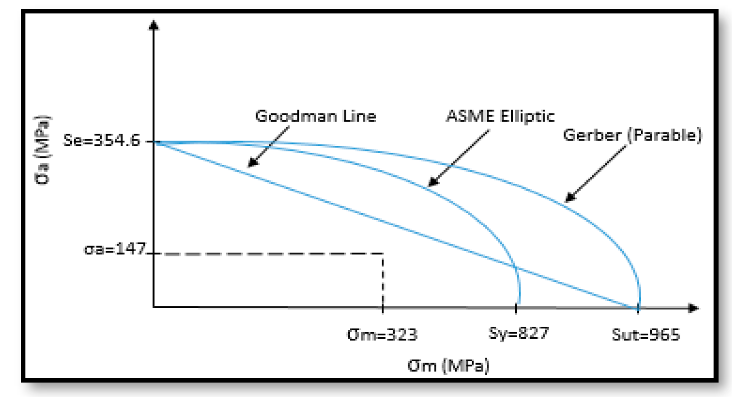
2.1. Static Stress Analysis
3. Proposed Method
3.1. Generalities of the Weibull Analysis
3.2. Weibull Stress Family Estimation and Its Random Behavior Analysis
3.3. Weibull Cycle Family Estimation and Its Random Behavior
3.3.1. Estimation of the N Value that Corresponds to the Equivalent Stress Value
3.3.2. Determination of the Weibull Cycle Parameters
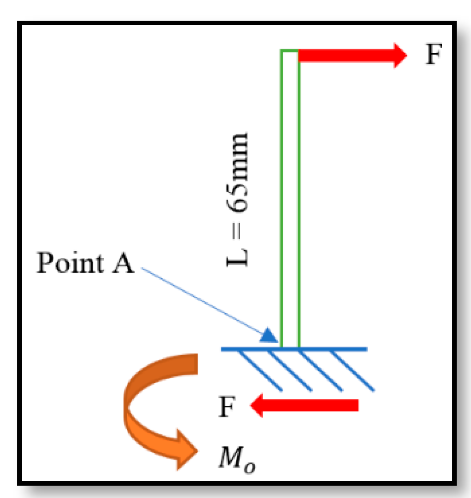
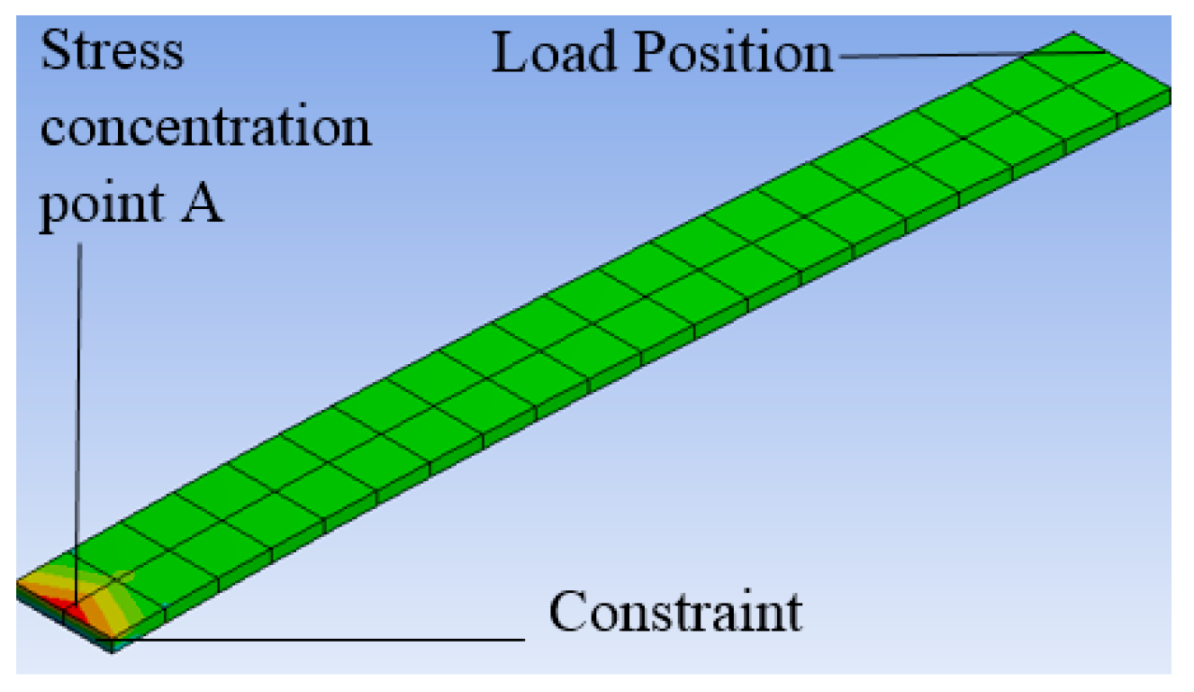
4. Mechanical Application with Weibull/Finite Element Analysis (FEA)
4.1. Weibull FEA Stress Data Analysis
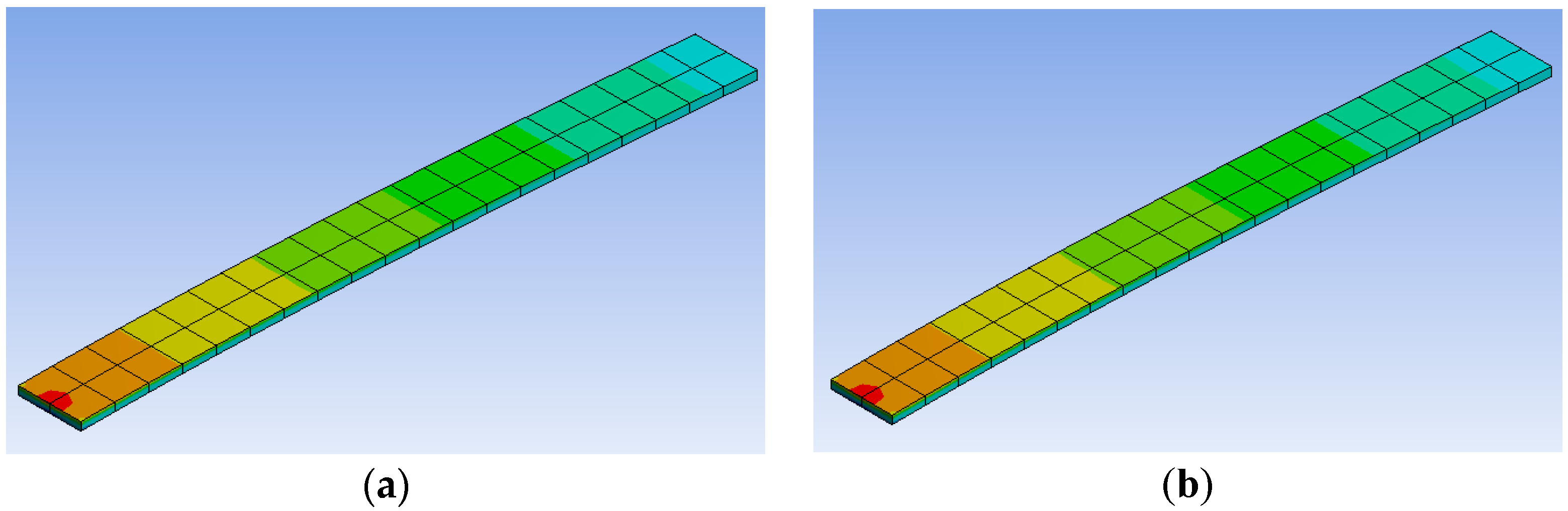
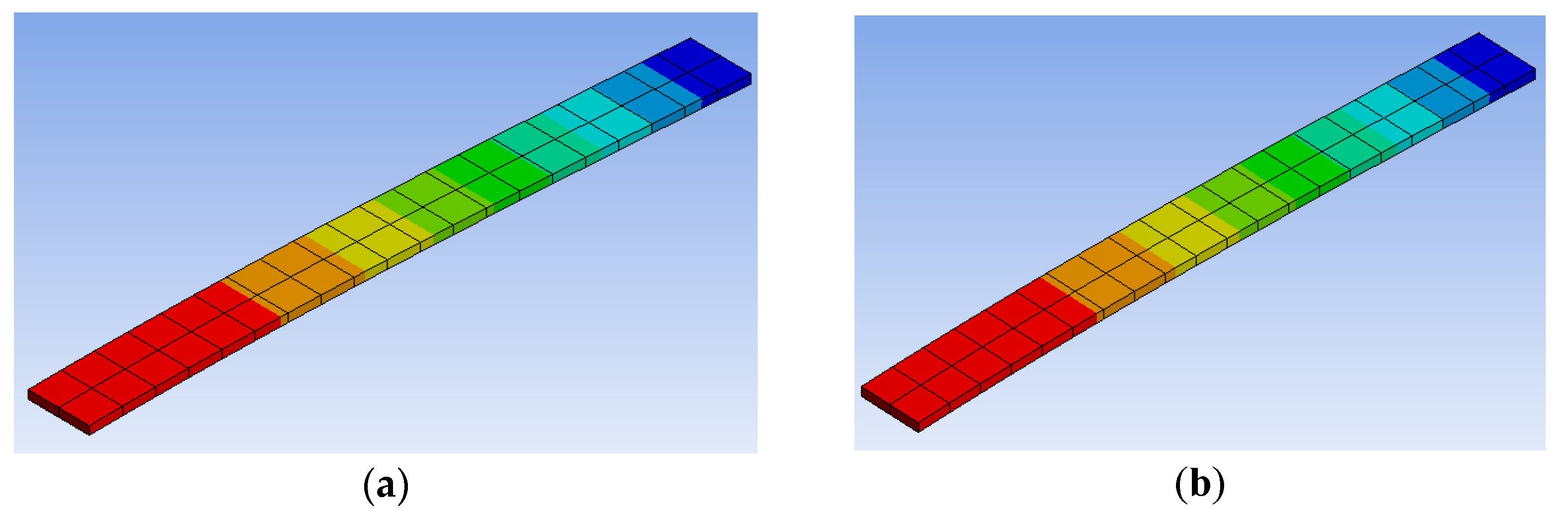
4.1.1. Validation of the Applied Principal Stresses σ1 and σ2 Values
4.1.2. Weibull Stress Family Determination
4.1.3. Stress Random Behavior
4.2. Weibull Cycle to Failure (N) Analysis
4.2.1. Weibull Cycle Parameters
4.2.2. Cycle Random Behavior
4.2.3. Weibull Stress Analytical Static Family
5. Conclusions
- Because the input’s method are the and values, then the proposed method can be applied in any mechanical analysis where and are known.
- The efficiency of the proposed method is that the Weibull (see Equations (8)) and (see Equation (9)) only depends on the and values. Consequently, by performing the Weibull analysis we can always reproduce them (see row between rows 5 and 6 Table 4).
- In the proposed method the mechanical element reliability can be determined by either the stress values (see column in Table 5) or by the corresponding cycle to failure values.
- The random behavior of both and values is determined based on the and on the its corresponding value, here determined by Basquin’s equation, but if they are determined in any other form the proposed method will be also efficient at determining the random behavior around them.
- As demonstrated in [14], the standard fatigue methodologies based on the stress-strain analysis and on the mechanical fracture both converge to the same solution; it might then be possible to extend the proposed method to be used in the strain and mechanical fracture analysis by related the equivalent stress to the total deformation given by the elastic (Basquin’s equation) and plastic (Coffin–Mason equation) areas, although further research should be undertaken.
Author Contributions
Funding
Conflicts of Interest
References
- Fatemi, A.; Yang, L. Cumulative fatigue damage and life prediction theories: A survey of the state of the art for homogeneous materials. Int. J. Fatigue 1998, 20, 9–34. [Google Scholar] [CrossRef]
- Nakada, M.; Miyano, Y. Statistical Creep Failure Time of Unidirectional CFRP. Exp. Mech. 2015, 56, 653–658. [Google Scholar] [CrossRef]
- Burhan, I.; Kim, H.S. S-N Curve Models for Composite Materials Characterisation: An Evaluative Review. J. Compos. Sci. 2018, 2, 38. [Google Scholar] [CrossRef]
- Hotait, M.A.; Kahraman, A. Estimation of Bending Fatigue Life of Hypoid Gears Using a Multiaxial Fatigue Criterion. J. Mech. Des. 2013, 135, 101005. [Google Scholar] [CrossRef]
- Polak, T. Machine elements in mechanical design. Tribol. Int. 1987, 20, 107. [Google Scholar] [CrossRef]
- Budynas, R.; Nisbett, J. Shigley’s Mechanical Engineering Design, 10th ed.; McGraw Hill: New York, NY, USA, 2015. [Google Scholar]
- Sága, M.; Blatnická, M.; Blatnický, M.; Dižo, J.; Gerlici, J. Research of the Fatigue Life of Welded Joints of High Strength Steel S960 QL Created Using Laser and Electron Beams. Materials 2020, 13, 2539. [Google Scholar] [CrossRef]
- Novak, J.S.; De Bona, F.; Benasciutti, D. Benchmarks for Accelerated Cyclic Plasticity Models with Finite Elements. Metals 2020, 10, 781. [Google Scholar] [CrossRef]
- Močilnik, V.; Gubeljak, N.; Predan, J. Effect of Residual Stresses on the Fatigue Behaviour of Torsion Bars. Metals 2020, 10, 1056. [Google Scholar] [CrossRef]
- Garivaltis, D.S.; Garg, V.K.; D’Souza, A.F. Fatigue Damage of the Locomotive Suspension Elements under Random Loading. J. Mech. Des. 1981, 103, 871–880. [Google Scholar] [CrossRef]
- Castillo, E.F.; Canteli, A.F. A general regression model for lifetime evaluation and prediction. Int. J. Fract. 2001, 107, 117–137. [Google Scholar] [CrossRef]
- Harikrishnan, R.; Mohite, P.; Upadhyay, C. Generalized Weibull model-based statistical tensile strength of carbon fibres. Arch. Appl. Mech. 2018, 88, 1617–1636. [Google Scholar] [CrossRef]
- Méndez-González, L.C.; Rodríguez-Picón, L.A.; Valles-Rosales, D.J.; Iniesta, A.A.; Carreón, A.E.Q. Reliability analysis using exponentiated Weibull distribution and inverse power law. Qual. Reliab. Eng. Int. 2019, 35, 1219–1230. [Google Scholar] [CrossRef]
- Castillo, A. Enrique; Fernandez-Canteli, a Unified Statistical Methodology for Modeling Fatigue Damage; Springer: Berlin/Heidelberg, Germany, 2009. [Google Scholar]
- Hedan, S.; Valle, V.; Cottron, M. In Plane Displacement Formulation for Finite Cracked Plates under Mode I Using Grid Method and Finite Element Analysis. Exp. Mech. 2009, 50, 401–412. [Google Scholar] [CrossRef]
- Wang, H.; Kim, N.H.; Kim, Y.-J. Safety Envelope for Load Tolerance and its Application to Fatigue Reliability Design. J. Mech. Des. 2005, 128, 919–927. [Google Scholar] [CrossRef][Green Version]
- Armentani, E.; Greco, A.; De Luca, A.; Sepe, R. Probabilistic Analysis of Fatigue Behavior of Single Lap Riveted Joints. Appl. Sci. 2020, 10, 3379. [Google Scholar] [CrossRef]
- Chang, H.; Shen, M.; Yang, X.; Hou, J. Uncertainty Modeling of Fatigue Crack Growth and Probabilistic Life Prediction for Welded Joints of Nuclear Stainless Steel. Materials 2020, 13, 3192. [Google Scholar] [CrossRef]
- Marsh, G.; Wignall, C.; Thies, P.R.; Barltrop, N.; Incecik, A.; Venugopal, V.; Johanning, L. Review and application of Rainflow residue processing techniques for accurate fatigue damage estimation. Int. J. Fatigue 2016, 82, 757–765. [Google Scholar] [CrossRef]
- Lee, Y.-L.; Pan, J.; Hathaway, R.B.; Barkey, M.E. Fatigue Testing and Analysis: Theory and Practice; Elsevier Butterworth-Heinemann: Burlington, MA, USA, 2005. [Google Scholar]
- Bandara, C.S.; Siriwardane, S.C.; Dissanayake, U.I.; Dissanayake, R. Developing a full range S–N curve and estimating cumulative fatigue damage of steel elements. Comput. Mater. Sci. 2015, 96, 96–101. [Google Scholar] [CrossRef]
- Blacha, Ł.; Karolczuk, A. Validation of the weakest link approach and the proposed Weibull based probability distribution of failure for fatigue design of steel welded joints. Eng. Fail. Anal. 2016, 67, 46–62. [Google Scholar] [CrossRef]
- Weibull, W. A Statistical Theory of the Strength of Materials. In Generalstabens Litografiska Anstalts Förlag; Centraltryckeriet: Stockholm, Sweden, 1939. [Google Scholar]
- Piña-Monarrez, M.R. Weibull stress distribution for static mechanical stress and its stress/strength analysis. Qual. Reliab. Eng. Int. 2017, 34, 229–244. [Google Scholar] [CrossRef]
- AmesWeb. 2019. Available online: https://www.amesweb.info/Stress-Strain/Theories-of-Failure-.for-Ductile-Materials.aspx (accessed on 26 February 2019).
- Mischke, C.R. A distribution—Independent plotting rule for ordered failures. J. Mech. Des. 1979, 104, 593–597. [Google Scholar] [CrossRef]
- Pucknat, D.; Liebich, R. A damage tolerance analysis for complex structures. Arch. Appl. Mech. 2015, 86, 669–686. [Google Scholar] [CrossRef]
- American Welding Society, Structural Welding Code-Steel; ANSI/AWS D1.1/D1.1M:2020. 2020. Available online: https://pubs.aws.org/Download_PDFS/AWS_D1_1_D1_1M_2020-PV.pdf (accessed on 23 April 2020).
- Mi, C.; Li, W.; Xiao, X.; Berto, F. An Energy-Based Approach for Fatigue Life Estimation of Welded Joints without Residual Stress through Thermal-Graphic Measurement. Appl. Sci. 2019, 9, 397. [Google Scholar] [CrossRef]
- Francesconi, L.; Baldi, A.; Dominguez, G.; Taylor, M. An Investigation of the Enhanced Fatigue Performance of Low-porosity Auxetic Metamaterials. Exp. Mech. 2019, 60, 93–107. [Google Scholar] [CrossRef]


| Maximum Principal Stress (MPa) Force F1 = 4.63 N | Minimum Principal Stress (MPa) Force F2 = 1.74 N | Deformation (mm) Force F1 = 4.63 N | Deformation (mm) Force F2 = 1.74 N |
|---|---|---|---|
| 491.75 | 184.8 | 8.02 | 2.99 |
| Application | Maximum Principal Stress (MPa), Force F1 = 4.63 N | Minimum Principal Stress (MPa), Force F2 = 1.74 N | Deformation (mm) Force F1 = 4.63 N | Deformation (mm) Force F2 = 1.74 N |
|---|---|---|---|---|
| Static | 470 | 176 | 8.00 | 3.00 |
| FEA | 491.75 | 184.8 | 8.02 | 2.99 |
| Parameter | Condition to Be Met for Safe Design | Status | |
|---|---|---|---|
| Maximum Shear Stress | 491.8 < 501.8 | Ok | |
| Distortion Energy | 430.2 < 501.2 | Ok | |
| n Equation (13) | Yi Equation (15) | toi Equation (17) | R(toi) Equation (22) | σ2i Equation (18) | σ1i Equation (19) | σmed Equation (25) | σalt Equation (26) | σeq (ASME) Equation (29) |
|---|---|---|---|---|---|---|---|---|
| 1 | −3.4034833 | 0.220104 | 0.96729 | 66.35155 | 1308.124 | 687.2377 | 620.8861 | 1116.157138 |
| −2.9701952 | 0.26688 | 0.95 | 80.45246 | 1078.849 | 579.6507 | 499.1982 | 699.8903536 | |
| 2 | −2.491662 | 0.330174 | 0.920561 | 99.53286 | 872.034 | 485.7834 | 386.2506 | 477.2687796 |
| −2.2691664 | 0.364517 | 0.901768 | 109.8856 | 827 | 468.4428 | 358.5572 | 435.0865005 | |
| 3 | −2.0034632 | 0.410239 | 0.873832 | 123.6689 | 701.842 | 412.7555 | 289.0865 | 333.6083957 |
| 4 | −1.6616459 | 0.477593 | 0.827103 | 143.9731 | 602.8627 | 373.4179 | 229.4448 | 257.1517697 |
| 5 | −1.3943983 | 0.537869 | 0.780374 | 162.1435 | 535.3039 | 348.7237 | 186.5802 | 205.7685332 |
| −1.0845459 | 0.617339 | 0.713156 | 184.8 | 491.75 | 338.275 | 153.475 | 168.1886402 | |
| 6 | −1.1720537 | 0.593774 | 0.733645 | 178.9966 | 484.9034 | 331.95 | 152.9534 | 166.9966579 |
| 7 | −0.9793812 | 0.646898 | 0.686916 | 195.0109 | 445.0831 | 320.047 | 125.0361 | 135.6021558 |
| 8 | −0.8074473 | 0.698303 | 0.640187 | 210.5073 | 412.3183 | 311.4128 | 100.9055 | 108.9229489 |
| 9 | −0.6504921 | 0.748789 | 0.593458 | 225.7266 | 384.5185 | 305.1225 | 79.39597 | 85.4226406 |
| 10 | −0.5045088 | 0.799016 | 0.546729 | 240.8679 | 360.3471 | 300.6075 | 59.73961 | 64.12598946 |
| 11 | −0.3665129 | 0.84959 | 0.5 | 256.1134 | 338.8969 | 297.5051 | 41.39172 | 44.36161829 |
| 12 | −0.2341223 | 0.901115 | 0.453271 | 271.6459 | 319.519 | 295.5825 | 23.93655 | 25.62949661 |
| 13 | −0.1052851 | 0.954255 | 0.406542 | 287.6654 | 301.7256 | 294.6955 | 7.030101 | 7.524013293 |
| 0 | 1 | 0.367879 | 301.4555 | 301.4555 | 301.4555 | 0 | 0 | |
| 14 | 0.0219284 | 1.0098 | 0.359813 | 304.4098 | 285.129 | 294.7694 | 9.640397 | 10.31807533 |
| 15 | 0.14952577 | 1.068761 | 0.313084 | 322.1837 | 269.3992 | 295.7915 | 26.39226 | 28.26181481 |
| 16 | 0.279845 | 1.132534 | 0.266355 | 341.4085 | 254.2293 | 297.8189 | 43.58962 | 46.7245514 |
| 17 | 0.4159621 | 1.203211 | 0.219626 | 362.7145 | 239.2957 | 301.0051 | 61.70939 | 66.25374946 |
| 18 | 0.56250196 | 1.284238 | 0.172897 | 387.1405 | 224.1978 | 305.6691 | 81.47139 | 87.68037713 |
| 19 | 0.72761583 | 1.382091 | 0.126168 | 416.639 | 208.3243 | 312.4817 | 104.1573 | 112.4970518 |
| 20 | 0.92931067 | 1.511797 | 0.079439 | 455.7394 | 190.451 | 323.0952 | 132.6442 | 144.096238 |
| 21 | 1.22965981 | 1.727846 | 0.03271 | 520.8685 | 166.6371 | 343.7528 | 177.1157 | 194.7355493 |
| n Equation (13) | Yi Equation (15) | toi Equation (17) | R(toi) Equation (22) | σ2i Equation (18) | σ1i Equation (19) | N (Cycles) Equation (33) |
|---|---|---|---|---|---|---|
| 1 | −3.4034833 | 0.220104 | 0.96729 | 66.35155 | 1308.124 | 273,683,422.9 |
| −2.9701952 | 0.26688 | 0.95 | 80.45246 | 1078.849 | 331,846,104.7 | |
| 2 | −2.491662 | 0.330174 | 0.920561 | 99.53286 | 872.034 | 410,547,979.5 |
| −2.2691664 | 0.364517 | 0.901768 | 109.8856 | 827 | 453,250,454.5 | |
| 3 | −2.0034632 | 0.410239 | 0.873832 | 123.6689 | 701.842 | 510,103,112.7 |
| 4 | −1.6616459 | 0.477593 | 0.827103 | 143.9731 | 602.8627 | 593,852,935.8 |
| 5 | −1.3943983 | 0.537869 | 0.780374 | 162.1435 | 535.3039 | 668,801,050.2 |
| −1.0845459 | 0.617339 | 0.713156 | 184.8 | 491.75 | 767,615,910 | |
| 6 | −1.1720537 | 0.593774 | 0.733645 | 178.9966 | 484.9034 | 738,315,719.9 |
| 7 | −0.9793812 | 0.646898 | 0.686916 | 195.0109 | 445.0831 | 804,370,622.7 |
| 8 | −0.8074473 | 0.698303 | 0.640187 | 210.5073 | 412.3183 | 868,289,756.6 |
| 9 | −0.6504921 | 0.748789 | 0.593458 | 225.7266 | 384.5185 | 931,065,175.7 |
| 10 | −0.5045088 | 0.799016 | 0.546729 | 240.8679 | 360.3471 | 993,519,280.8 |
| 11 | −0.3665129 | 0.84959 | 0.5 | 256.1134 | 338.8969 | 1,056,403,357 |
| 12 | −0.2341223 | 0.901115 | 0.453271 | 271.6459 | 319.519 | 1,120,470,957 |
| 13 | −0.1052851 | 0.954255 | 0.406542 | 287.6654 | 301.7256 | 1,186,547,445 |
| 0 | 1 | 0.367879 | 301.4555 | 301.4555 | 1,243,427,849 | |
| 14 | 0.0219284 | 1.0098 | 0.359813 | 304.4098 | 285.129 | 1,255,613,543 |
| 15 | 0.14952577 | 1.068761 | 0.313084 | 322.1837 | 269.3992 | 1,328,926,684 |
| 16 | 0.279845 | 1.132534 | 0.266355 | 341.4085 | 254.2293 | 1,408,224,098 |
| 17 | 0.4159621 | 1.203211 | 0.219626 | 362.7145 | 239.2957 | 1,496,105,985 |
| 18 | 0.56250196 | 1.284238 | 0.172897 | 387.1405 | 224.1978 | 1,596,857,176 |
| 19 | 0.72761583 | 1.382091 | 0.126168 | 416.639 | 208.3243 | 1,718,530,710 |
| 20 | 0.92931067 | 1.511797 | 0.079439 | 455.7394 | 190.451 | 1,879,810,288 |
| 21 | 1.22965981 | 1.727846 | 0.03271 | 520.8685 | 166.6371 | 2,148,451,296 |
| Application | Maximum Principal Stress (MPa), Force F1 = 4.63 N | Minimum Principal Stress (MPa), Force F2 = 1.74 N | Weibull β Parameter | Cycles to Failure (N) | Reliability R(t) |
|---|---|---|---|---|---|
| Static | 470 | 176 | 2.240388 | 691,910,584 | 0.91 |
| FEA | 491.75 | 184.8 | 2.248519 | 453,250,454 | 0.90 |
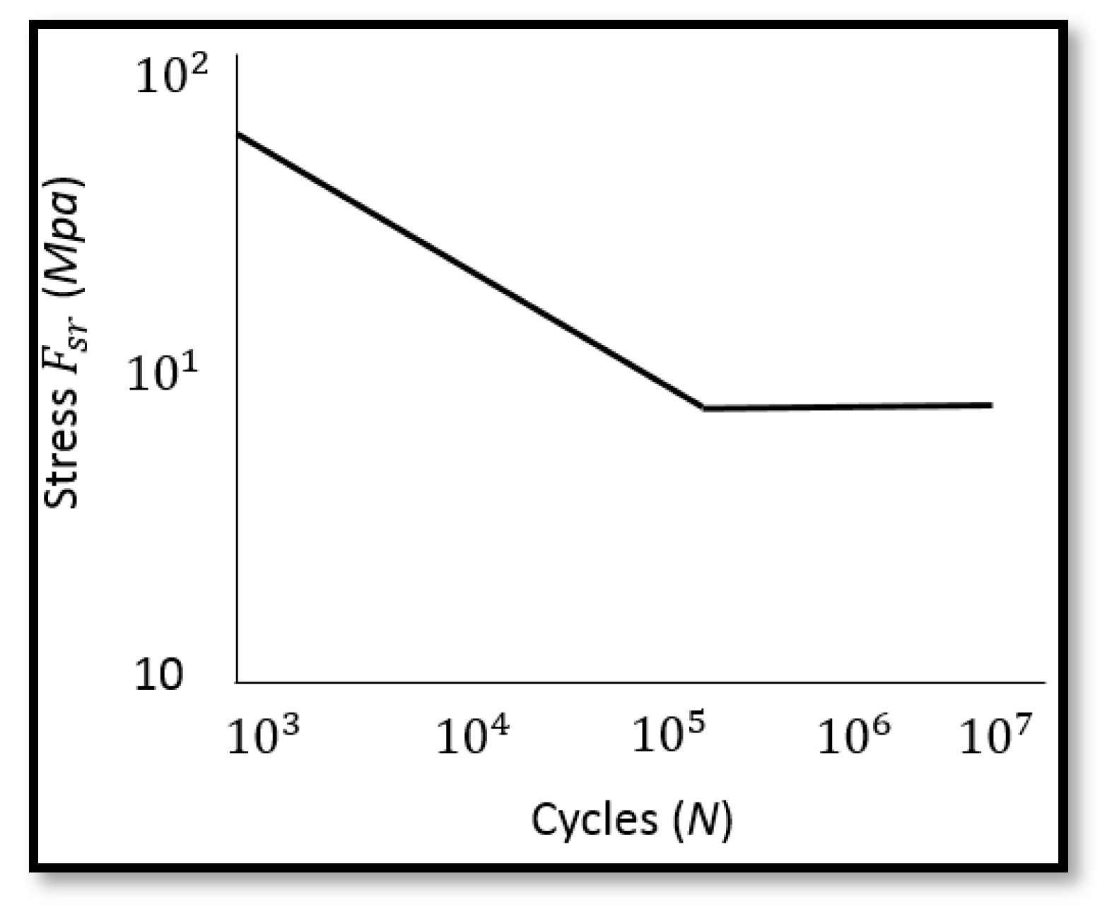
| Application | Allowable Stress Range FSR (MPa) Equation (37) | Cycles to Failure (N) Equation (36) | Reliability R(t) |
|---|---|---|---|
| Static | 294 | 155,358 | 0.91 |
| FEA | 307 | 136,446 | 0.90 |
© 2020 by the authors. Licensee MDPI, Basel, Switzerland. This article is an open access article distributed under the terms and conditions of the Creative Commons Attribution (CC BY) license (http://creativecommons.org/licenses/by/4.0/).
Share and Cite
Barraza-Contreras, J.M.; Piña-Monarrez, M.R.; Molina, A. Fatigue-Life Prediction of Mechanical Element by Using the Weibull Distribution. Appl. Sci. 2020, 10, 6384. https://doi.org/10.3390/app10186384
Barraza-Contreras JM, Piña-Monarrez MR, Molina A. Fatigue-Life Prediction of Mechanical Element by Using the Weibull Distribution. Applied Sciences. 2020; 10(18):6384. https://doi.org/10.3390/app10186384
Chicago/Turabian StyleBarraza-Contreras, Jesús M., Manuel R. Piña-Monarrez, and Alejandro Molina. 2020. "Fatigue-Life Prediction of Mechanical Element by Using the Weibull Distribution" Applied Sciences 10, no. 18: 6384. https://doi.org/10.3390/app10186384
APA StyleBarraza-Contreras, J. M., Piña-Monarrez, M. R., & Molina, A. (2020). Fatigue-Life Prediction of Mechanical Element by Using the Weibull Distribution. Applied Sciences, 10(18), 6384. https://doi.org/10.3390/app10186384