Accurate Bearing Fault Diagnosis under Variable Shaft Speed using Convolutional Neural Networks and Vibration Spectrogram

Abstract

Predicting bearing faults is an essential task in machine health monitoring because bearings are vital components of rotary machines, especially heavy motor machines. Moreover, indicating the degradation level of bearings will help factories plan maintenance schedules. With advancements in the extraction of useful information from vibration signals, diagnosis of motor failures by maintenance engineers can be gradually replaced by an automatic detection process. Especially, state-of-the-art methods using deep learning have contributed significantly to automatic fault diagnosis. This paper proposes a novel method for diagnosing bearing faults and their degradation level under variable shaft speed. In the proposed method, vibration signals are represented by spectrograms to apply deep learning methods through preprocessing using Short-Time Fourier Transform (STFT). Then, feature extraction and health status classification are performed by a convolutional neural network (CNN), VGG16. According to our various experiments, our proposed method can achieve very high accuracy and robustness for bearing fault diagnosis even under noisy environments.

1. Introduction

Vibration monitoring for rotary machines tracks important components in the time between planned maintenance. The monitoring process helps factories prevent severe damage to electrical machines, ensure product quality, and have active plans in the production process. Vibration signals emitted from electrical motor systems contain health information about these systems that can detect potential damage. According to a literature review, 40–50% of electric motor failures occur due to bearing faults [1]. Especially in heavy motor machines, it is critical to find broken components that need repair or replacement. Moreover, indicating the degradation level of the component will help plan the time of repair.

Vibration-based bearing fault diagnosis is adopted early by using signal representation methods independently in the time or frequency domains. For example, envelope analysis can be used to show the tendency of signals in the frequency domain [2]. From the change of the spectrum envelope, bearing faults can be predicted through observation by maintenance engineers. With advancements in the study of extracting useful information from vibration signals, diagnosis of motor failures by maintenance engineers can be gradually replaced by an automatic process. Recent automatic diagnosis methods have focused on achieving high accuracy and flexibility. However, in those methods, very complex fault diagnosis processes are required to analyze the acquired vibration signals.

When the characteristics of signals tend to be nonstationary, time-frequency approaches become appropriate and reach high efficiency. Improved Hilbert–Huang transforms (HHT) illustrated that it is a potential computation-efficient time-frequency method and is unaffected by frequency resolution and time resolution compared to wavelet-based scalogram, resulting in high-accuracy detection for rolling bearing faults by using vibration signals [3]. Empirical mode decomposition (EMD) to decompose the number of intrinsic mode functions (IMFs) was also proposed to improve diagnosis accuracy [4]. A third-order statistic bi-spectrum was applied to analyze and detect single-bearing fault types. Moreover, intelligent algorithms and techniques such as support vector machines (SVMs) and artificial neural networks (ANNs) also enhance the prediction accuracy for bearing faults. After using Discrete wavelet transform (DWT) as preprocessing for feature extraction, the SVM classifier fed by determined statistic features performs better than ANN in detecting bearing faults [5].

Over the last few years, the development of convolutional neural networks (CNNs) for artificial intelligence has improved the accuracy of fault diagnosis significantly, where various kinds of features affect the diagnosis process. The method using CNN as a back-end classifier and training it by statistics features extracted from vibration signals of single faults provides high accuracy for fault diagnosis [6]. More recent studies have also achieved high diagnosis accuracy by using CNNs for the bearing faults. D. T. Hoang and H. J. Kang used vibration signals directly as the input data for bearing fault diagnosis by adopting an automatic fault diagnosis system that does not require any feature extraction techniques, which achieved high accuracy and robustness under noisy environments while considering variable shaft speeds [7].

In a real fault diagnosis process, there are situations in which a covariate is not directly measured, thereby confounding the diagnosis of machines. To improve the accuracy of fault diagnosis methods based on deep learning, especially CNNs, constructing nonlinear representations automatically under complex situations is very important. Therefore, the studies that apply CNNs after the preprocessing stage have achieved high prediction accuracy even under complex working conditions. When classifying bearing cracks of multiple scales and compound faults at variable shaft speeds, using bi-spectrum images to represent signals achieved high accuracy [8]. A CNN with the Adamax optimizer was used to extract the features and to classify types of compounds bearing faults. The efficiency of combining CNN and the time-frequency representation was also proved by using HHT to create time-frequency images as input data for CNN [9].

Meanwhile, the spectrogram is a simple method that represents useful information from nonstationary signals [10]. In order to classify bearing faults under complicated conditions, a deep enough CNN network is required. Thus, our study aims to apply a deep and capable CNN model with spectrograms by preprocessing to obtain high accuracy even under complex working conditions. This paper proposes a new fault diagnosis method using a practical CNN to extract useful information from signal representation in the time-frequency domain. The proposed method can achieve high accuracy in diagnosing compound bearing faults under variable shaft speeds. In addition, the stability of the proposed method under noisy environments is also proved through various experiments. The remainder of this paper is organized as follows. Section 2 presents the details of our proposed bearing fault diagnosis method, and Section 3 presents the detailed experimental methods. Section 4 provides a discussion of various experimental results, and Section 5 presents the conclusions.

2. Proposed Bearing Fault Diagnosis Method

An overview of the proposed bearing fault diagnosis method is shown in Figure 1. First, the vibration signals are split into fixed-cycle 5 seconds segments. The Short-Time Fourier Transform (STFT) is then applied for each signal segment to produce the spectrogram. Then, spectrogram images generated from the vibration signals corresponding to the bearing faults are used to train network architecture CNN-VGG16, and the trained CNN-VGG16 model is used to classify bearing faults automatically in the test stage.

2.1. Signal Preprocessing

The vibration signals acquired from electrical machines are nonstationary as they contain bearing fault information modulated for variable rotational speeds and surrounding environmental noise. The frequency of the obtained signal is continuous, and its time-domain statistical features change with time. Nonstationary signals typically lack useful information in the time or frequency domains but may have useful information through merge representation within the time-frequency $\left(t, f\right)$ space.

In varying working conditions of bearings (various types of single and compound faults and various degradation levels at variable rotational speeds), traditional signal processing methods such as envelope spectrum analysis and wavelet package transform are challenging to obtain meaningful information. Under these conditions, the signal’s spectrum varies greatly in amplitude and frequency. Therefore, it is troublesome to recognize the deficiencies of bearings under adverse working conditions using conventional signal processing methods. For appropriate analysis and synthesis of nonstationary signals, Short-Time Fourier Transform (STFT) is a typical Fourier transform (FT) applied to create the spectrograms of signals. The spectrogram is a visual representation of the signals in both the time and frequency domains, using a color scale of the image to indicate the frequency’s amplitude.

2.1.1. Short-Time Fourier Transform

STFT applies a Fourier transform for localization both in the frequency and time domains for signals that are time-varying or nonstationary [11]. The process for the STFT can be represented as follows.

$$x_1\left[m\right]=x[m+\mathit{lH}]w\left[m\right]$$

(1)

where m ∈ M {1, 2, …} is an index related to the beginning of the sliding extraction window (local time index), M ∈ N is the analysis window length, l ∈ {0, 1, …, L – 1} is the frame index, L ∈ N is the number of frames, and H ∈ N is the hop size. Further, the following discrete Fourier transform (DFT) is performed on every frame $x_1[m]$ given a localized two-sided spectrum [11]:

$$\dot{X}[k,l]=\frac{1}{M}{\displaystyle \sum _{m-1}^k{x}_i{\left[m\right]e}^{-\frac{j2\pi \mathit{mk}}{K}}}$$

(2)

where k ∈ {1, 2, …, K} is the frequency bin index and K ∈ N is the DFT size.

The term $\dot{X}[k,l]$ is called the STFT of $x \left[n\right]$ and corresponds to the local time-frequency behavior of the signal around the time index $lH$ and frequency bin k.

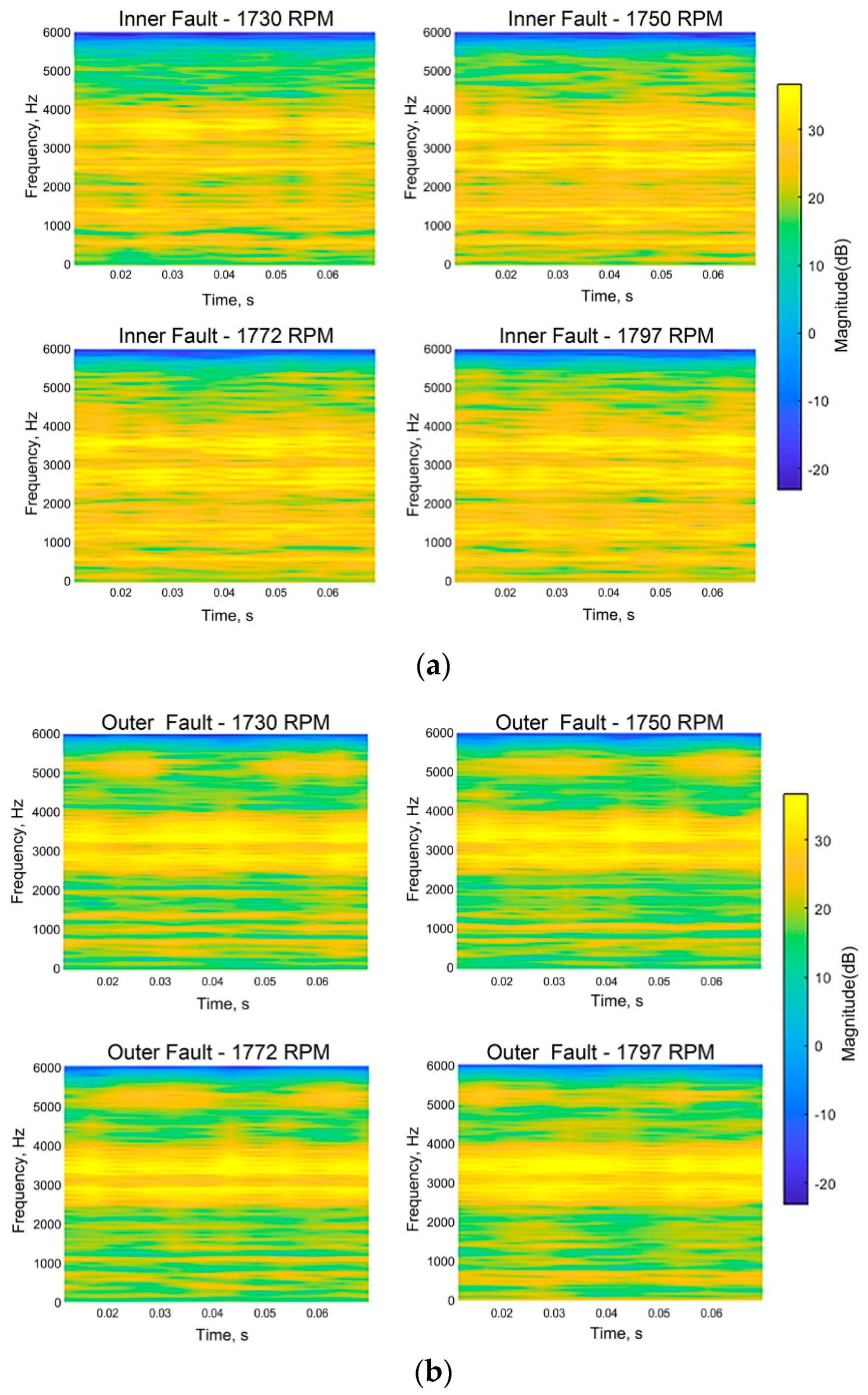
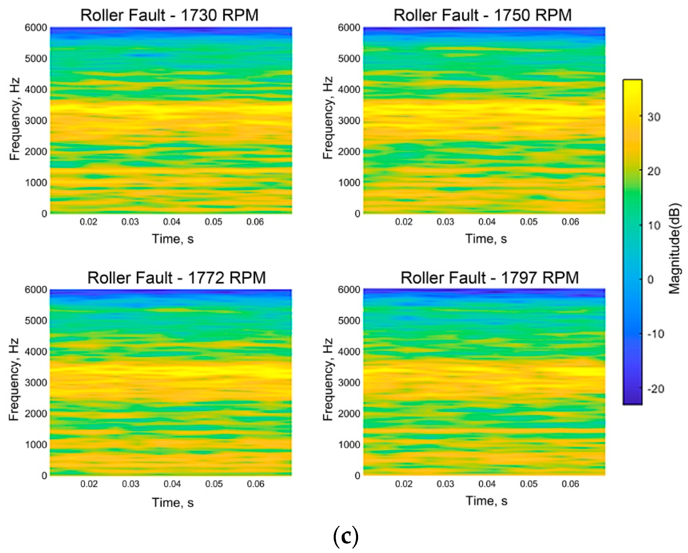
2.1.2. Implementing STFT Analysis for Spectrograms

With the advantages of frequency-domain analysis for nonstationary signals, STFT can be a good approach for analyzing the bearing signals under complex conditions or with background noise. To efficiently apply STFT to bearing fault signals, the STFT matrix can be determined by a new routine with the MATLAB tool to achieve high accuracy and computational efficiency [12]. After analyzing which segment duration of the signal has essential features (such as mean, RMS, standard deviation, variance, kurtosis, skewness, crest factor, and form factor that do not change with time), the window length ($wlen$) is set as 1024. The accuracy is prioritized to $wlen$, although the shorter windows affect the calculation volume in a negative manner. The hop size is set to $wlen$/4 based on various experiments [12]. Figure 2 shows the spectrograms produced by applying STFT to vibrations signals with four different shaft speeds (1730, 1750, 1772, and 1797 RPM) with three kinds of faults (inner race fault, outer race fault, and roller fault).

2.2. CNN-VGG16 Model for Bearing Fault Classification

The CNN architecture affects prediction accuracy and calculation volumes. If an efficient CNN network is selected, it can achieve high prediction accuracy while optimizing the calculation volume. Therefore, a practical model should be used for the systems with limited hardware. Typically, the design and selection of a CNN network architecture should focus on the structure of the network and its size (resolution of input data and the width and depth of the CNN). The complexity level of the CNN architecture is chosen based on the characteristics of the input data and the number of output neurons (the number of layers to be classified). Currently, there are many research results for new CNN network architectures that are highly effective in image classification. The choice of network architecture ensures high prediction accuracy with the most optimal resources. For accurate bearing fault diagnosis, we examined various scenarios based on the architecture using VGG16 [13].

A CNN model with a limited number of layers is economical considering storage and computing resources. However, for solutions to complex problems such as diagnosing various types of faults under changing rotational speed conditions, a deeper CNN needs to be applied. Previous studies applied generic structuring CNNs, which consist of convolutional layers, pooling layers, and fully connected layers [14]. LeNet-5, which is constructed by five simple CNN layers, was used for bearing fault diagnosis [15,16]. Similarly, a simple self-designed CNN with two CNN layers was also proposed [8].

Although simple structuring CNN architectures are easy to design and do not require many computation resources, novel complex CNN architectures using efficient techniques can provide high fault diagnosis accuracy in complicated scenarios. VGG16 is a potential model that focuses on depth while previous bearing fault diagnosis methods using the AlexNet CNN model focused on tiny window sizes and strides, in particular, convolutional layers [9,17]. The VGG16 model has been proven beneficial to classification accuracy.

Figure 3 shows the detailed architecture of our VGG16 model fed by spectrogram images. The input size of the proposed VGG16 is fixed at 224 × 224 with 3 channels (RGB images). The input image is transmitted through the vast majority of convolution layers where the filters are applied with their receiver field which is very small: 3 × 3. In other configurations, it also uses a built-in smaller size: 1 × 1. The design of those tiny filters acts as a linear transformation of the input image channels (followed by a nonlinear transformation). The fixed size of the convolution strike is 1 pixel. The spatial padding of the input convolutional layer is preserved after convolution. Five max-pooling layers play the role of spatial pooling, which are added following convolutional layers to reduce their dimensionality. Max-pooling is performed over a 2 × 2 pixel window with a stride of 2. The following convolution layers are three fully connected (FC) layers. The first and second FC layers have 4096 neurons, and the number of neurons of the third FC layer depends on the number of different bearing faults needed to be classified (8 or 22 classes, depending on individual experiments). The final layer is the soft-max layer, which outputs a vector to show the prediction probability distribution for bearing faults. All hidden layers use rectification (ReLU) nonlinearity as an activation function [13].

3. Experimental Implementation

3.1. Single Faults Dataset

Bearing fault data from Case Western Reserve University (CWRU) were collected for single bearing faults and normal bearings of drive-end defects [18]. The accelerometer and acquisition system used to measure vibration signals were set at a sampling rate of 12 kHz. Defects having multiple crack sizes (0.007, 0.014, and 0.021 inches in diameter) occurred on the ball, outer raceway, and inner raceway. Moreover, the data were also collected at various shaft speeds (i.e., approximately 1722, 1748, 1772, and 1796 revolutions per minute (RPM)) caused by varying loads (i.e., 0, 1, 2, and 3 horsepower (hp)), from the testbed shown in Figure 4.

From CWRU data, we formulated four different datasets for the experiments, as depicted in

Table 1. Dataset for single bearing faults.

	Training Sample Speed (RPM)	Test Sample Speed (RPM)
Dataset 1	1796	(1772, 1748, 1722)
Dataset 2	1772	(1796, 1748, 1722)
Dataset 3	1748	(1772, 1796, 1722)
Dataset 4	1722	(1772, 1748, 1796)

. In each of those datasets, signal samples at a certain shaft speed were used for training CNN models. The number of samples for each bearing fault type at a certain crack size ($N_{Samples}$) was 80, the number of different crack sizes ($N_{Crack\_Size}$) was 3, and the number of bearing fault types ($N_{Class}{}_{es}$) was 4 (inner race bearing fault, outer race bearing fault, roller fault, and normal condition). Therefore, the total number of samples for training ($N_{Classes}\times N_{Crack\_size}\times N_{Samples}$) was 960.

On the other hand, signal samples at the rest of different shaft speeds were used for testing. For testing, the number of samples for each bearing fault type at a certain crack size and at a certain speed ($N_{Samples}$) was 40, the number of different crack sizes ($N_{Crack\_Size}$) was 3, the number of bearing fault type ($N_{Class}{}_{es}$) was 4, and the number of different shaft speeds used for testing ($N_{Speed}$) was 3. Therefore, the total number of samples used for testing ($N_{Class}{}_{es}\times N_{Crack\_size}\times N_{Samples}\times N_{speed}$) was 1440.

3.2. Compound Faults Dataset

Compound faults data was acquired from an electrical experiment system described by the diagram illustrated in Figure 5. The testbed was constructed by two rotational shafts: a drive-end shaft (DES) and a non-drive-end shaft (NDES) [8]. The DES and NDES were connected by a gearbox with a reduction ratio of 1.52:1. Rolling element bearings (FAG NJ206-E-TVP2) were installed at the ends of these shafts to alleviate the friction, which hampers movement. DES was activated by a three-phase induction motor at various shaft speeds (200, 250, 300, 350, 400, 450, and 500 RPM). As shown in Figure 6, bearings were seeded not only for a single-mode but also for compound faults of variable lengths of crack size: 3 mm, 6 mm, and 12 mm. The vibration signals were acquired by an acquisition system using a wideband vibration sensor sampling rate of 65,536 Hz mounted near the bearing at NDES, an amplifier (NEXUS condition amplifier type 2692-C), and a portable data acquisition device (PULSE type 3560-C). Specifications of the vibration accelerometer sensor and data acquisition system are shown in

Table 2. Specification of the data acquisition system.

NEXUS conditioning amplifier (type 2692-C)	(1) Frequency range: 0.1 Hz–100 kHz (2) Sensitivity: 10 mV/ms−2
Piezoelectric charge accelerometer (type 4371)	(1) Frequency range: 0.1 Hz–12.6 kHz (2) Sensitivity: 9.8pC/g
Portable data acquisition device (PULSE type 3560-C)	Maximum sampling frequency: 25.6 kHz

.

The recorded vibration signals are divided into three datasets. Each dataset consists of two separate subsets for the training and test stages. The training subset includes vibration signals acquired at shaft speeds of 300, 400, and 500 RPM, while the test subset includes vibration signals recorded at shaft speeds of 250, 350, and 450 RPM as described in

Table 3. Dataset for compound bearing faults.

		Rotational Speed (RPM)	Crack Size
			Length (mm)	Width (mm)	Depth (mm)
Dataset 5	Training dataset	300, 400, 500	3	0.60	0.30
	Test dataset	250, 350, 450
Dataset 6	Training dataset	300, 400, 500	6	0.60	0.50
	Test dataset	250, 350, 450
Dataset 7	Training dataset	300, 400, 500	12	0.60	0.50
	Test dataset	250, 350, 450

. Datasets 5, 6, and 7 consist of bearing fault samples at fixed crack sizes of 3 mm, 6 mm, and 12 mm. Hence, each of these datasets contains 5760 ($N_{Classes}\times N_{Samples}\times N_{Speed}$) vibration signals, where $N_{Speed}$ is 6, $N_{Classes}$ is 8, and $N_{Samples}$ is 120, since it denotes the total number of vibration signal samples recorded for each bearing condition at each shaft speed.

4. Experimental Results

4.1. Fault Diagnosis Accuracy for Single Bearing Faults

We conducted the experiments to evaluate the prediction accuracy for single bearing faults in our proposed method under variable motor speed conditions. These experiments were performed with datasets 1, 2, 3, and 4. The experimental results in

Table 4. Diagnosis accuracy of the proposed method for single faults compared to the method in the paper [8].

	Fault Diagnosis Method	Diagnosis Accuracy (Sensitivity, %)				Average Accuracy (%)
		Inner	Outer	Roller	Normal
Dataset 1	[8]	81.5	81.4	79.2	82.9	81.2
	Proposed method	98.1	99.1	98.2	100.0	98.8
Dataset 2	[8]	83.9	79.1	78.6	83.9	81.4
	Proposed method	97.6	100.0	100.0	100.0	99.4
Dataset 3	[8]	80.1	78.2	80.9	82.5	80.4
	Proposed method	96.3	99.6	100.0	99.6	98.9
Dataset 4	[8]	78.4	77.7	77.3	80.8	78.6
	Proposed method	98.1	100.0	100.0	99.2	99.3

show that the proposed method provides a high level of predictability compared to the existing high accuracy method, which uses the bi-spectrum to represent vibration signals and a shallow CNN model under the same conditions [8]. To obtain stable results, all of the experiments in this paper were repeated multiple times. Specifically, we repeated each of the experiments more than ten times and we found that the achieved results are consistent.

Sensitivity is the diagnosis ability to classify an individual fault correctly, which is one of the most important indicators to evaluate a diagnosis method and to compare its efficiency with other diagnostic methods. Therefore, most previous researches related to fault diagnosis have used the sensitivity value to evaluate performance. For this reason, we use the sensitivity value as the major index to evaluate and compare our method with previous methods. Sensitivity is calculated by the following Equation (3):

$$Sensitivity=\frac{N_{True\_Positive}}{N_{True\_Positive}+N_{False\_Negative}}\times 100(\%)$$

(3)

where $N_{True\_Positive}$ is the number of samples from a particular class which are correctly classified and $N_{False\_Negative}$ is the number of samples from a particular class that are incorrectly classified.

The average classification accuracy (ACA) is measured by Equation (4) to show the average classification performance for each dataset:

$$ACA=\frac{{\displaystyle \sum \mathit{Sensitivity}}}{{\displaystyle \sum N_{Classes}}}$$

(4)

where ${\displaystyle \sum \mathit{Sensitivity}}$ is the sum of class-wise accuracy for a specific dataset.

As shown in Table 4, for 4 bearing fault types (inner race bearing fault, outer race bearing fault, roller fault, and normal condition), our proposed method provides the average prediction accuracy 98.8, 99.4, 98.9, and 99.3% whereas the existing method provides the average accuracies 81.2, 81.4, 80.4, and 78.6% for datasets 1, 2, 3, and 4, respectively. Based on these results, we can know that our proposed bearing fault diagnosis method provides much higher prediction accuracy compared to the existing method for single bearing faults. Moreover, our bearing fault diagnosis method provides fast convergence ability (only 3 to 4 epochs for training), as shown in Figure 7.

4.2. Fault Diagnosis Accuracy for Compound Bearing Faults

We also evaluated the effectiveness of the proposed bearing fault diagnosis method by examining the prediction accuracy for seven types of localized defects (inner raceway crack (BCI), outer raceway crack (BCO), roller crack (BCR), inner and outer raceway cracks (BCIO), inner and roller cracks (BCIR), outer and roller cracks (BCOR), and inner-outer-roller cracks (BCIOR)) as recorded under variable operating speeds and fixed crack sizes of 3 mm, 6 mm, and 12 mm (datasets 5, 6, and 7). Figure 8a shows the diagnosis accuracy (sensitivity) of our proposed method for 3 single faults (BCI, BCO, and BCR), 4 combined faults (BCIO, BCIR, BCOR, and BCIOR), and the normal condition (BNC). Experimental results show that the proposed method exhibits high accuracy in the classification of single faults and combined faults independent of the rotational speed. Our method provides average accuracies of 96.3, 98.6, and 100% for datasets 5, 6, and 7, respectively. From these experimental results, we can know that our proposed bearing fault diagnosis method provides very high prediction accuracy for combined bearing faults as well as single bearing faults. In particular, the proposed method produces high and stable results when the bearing has a high level of degradation. For a 12-mm crack size, the proposed method provides an accuracy of up to 100%. The lowest average accuracy is 96.3% when the crack size is 3 mm.

Figure 9 presents the confusion matrices for the results to show the performance of the classification task corresponding to each class in detail. Each row of a confusion matrix represents the instances in a predicted label, while each column represents the instances in a true label. Confusion matrices are extremely practical to visualize the performance (sensitivity, precision, and accuracy) of the proposed method. Based on the confusion matrices, we additionally provide the precision values of individual classes in Figure 8b to show the performance of our proposed method on the full range of aspects. Precision is calculated by following Equation (5):

$$Precision=\frac{N_{True\_Positive}}{N_{True\_Positive}+N_{False\_Positive}}\times 100(\%)$$

(5)

where $N_{True\_Positive}$ is the number of samples from a particular class which are correctly classified and $N_{False\_Positive}$ is the number of outcomes where the model incorrectly predicts the positive class. The average precisions of our proposed method for datasets 5, 6, and 7 are 96.57, 98.38, and 99.83%, respectively. The evaluated high values both in sensitivity and precision prove that the proposed method performs well in bearing fault diagnosis.

Moreover, we calculated the computational costs for the two main methods used in our proposed diagnosis process in

Table 5. Computational costs for Short-Time Fourier Transform (STFT) and VGG16.

Algorithm	Computational Cost
STFT	218,000 (MAC)
VGG16	15.52 (GMAC)

, computational costs for STFT, and the computational costs for VGG16, where MAC unit denotes multiplier–accumulator.

4.3. Bearing Fault Diagnosis Accuracy in Noise Environments

We also evaluated the accuracy of our proposed bearing fault diagnosis method in noisy environments, which is common in industrial working conditions. In those cases, the vibration signals of compound faults are collected under shaft speed variation and a low level of signal-to-noise ratio (SNR). The vibration signal samples from three datasets above (datasets 5, 6, and 7) have three white noise levels added (SNR = 0, 5, and 10 dB). The SNR is defined as the ratio of the power of a signal (meaningful input) to the power of background noise:

$$SN{R}_{dB}=10{\log }_{10}\left(\frac{P_{signal}}{P_{noise}}\right)$$

(6)

Table 6. Diagnosis accuracy in noisy environments.

	SNR (dB)	Diagnosis Accuracy in Noisy Environments (%)								Average Accuracy (%)
		BCI	BCO	BCR	BCIO	BCIR	BCOR	BCIOR	BNC
Dataset 5	10	73.9	100.0	100.0	97.8	63.0	100.	100.00	95.7	91.3
	5	72.7	100.0	100.0	75.6	62.8	100.0	100.0	97.6	88.6
	0	73.9	97.8	95.6	73.9	52.2	100.0	100.0	89.1	85.3
Dataset 6	10	100.0	73.9	100	73.9	100.0	97.8	100.0	100	96.5
	5	100.0	78.3	100.0	97.8	100.0	95.7	100.0	97.8	96.2
	0	100.0	73.9	95.7	100.0	100.0	100.0	100.0	97.8	95.9
Dataset 7	10	97.7	100.0	100.0	100.0	100.0	100.0	100.0	100.0	99.7
	5	97.6	100.0	100.0	100.0	97.7	100.0	100.0	97.7	99.1
	0	97.6	100.0	100.0	100.0	97.6	100.0	100.0	93.2	98.6

provides the accuracy of our proposed bearing fault diagnosis method in noisy environments. It can be observed that noise degrades the accuracy of the proposed method, but it still provides high fault diagnosis accuracy. When the SNR values are positive, the average accuracy is higher than 98.6% when the crack size is 12 mm. The worst average accuracy is 85.3% when the crack size is 3 mm and SNR is 0.

5. Conclusions

We proposed a new fault diagnosis method for rotary machine bearings that can identify and recognize faults under inconsistent working conditions, including non-steady shaft speeds, bearings with cracks in different scales, compound faults, and noisy working environments. Moreover, the degradation level of every kind of bearing fault was evaluated to identify the diagnosis accuracy under complicated conditions. In the proposed bearing fault diagnosis method, spectrograms of vibration acceleration signals under inconsistent working conditions were calculated by the preprocessing using the Short-Time Fourier Transform (STFT), and then the spectrograms were provided as informative input data to the CNN model using VGG16 for fault identification and classification. Our proposed method provides average accuracy of almost 100% for combined bearing faults as well as single bearing faults. It means that representing nonstationary signals in the time-frequency domain can be a practical approach for bearing fault diagnosis using vibration signals. We also proved that the proposed method could predict bearing faults with very high accuracy even under noisy environments. Therefore, we can expect that the proposed method can be applied in real industrial environments under complex working conditions.

References

1. Albrecht, P.F.; Appiarius, J.C.; McCoy, R.M.; Owen, E.L.; Sharma, D.K. Assessment of the Reliability of Motors in Utility Applications-Updated. IEEE Trans. Energy Convers. 1986, EC-1, 39–46. [Google Scholar] [CrossRef]
2. McInerny, S.A.; Dai, Y. Basic vibration signal processing for bearing fault detection. IEEE Trans. Educ. 2003, 46, 149–156. [Google Scholar]
3. Peng, Z.K.; Tse, P.W.; Chu, F.L. A comparison study of improved Hilbert-Huang transform and wavelet transform: Application to fault diagnosis for rolling bearing. Mech. Syst. Signal Process. 2005, 19, 974–988. [Google Scholar] [CrossRef]
4. Saidi, L.; Ben Ali, J.; Fnaiech, F.; Morello, B. Bi-spectrum based-EMD applied to the non-stationary vibration signals for bearing faults diagnosis. ISA Trans. 2014, 53, 1650–1660. [Google Scholar] [CrossRef] [PubMed]
5. Tyagi, S. A DWT and SVM based method for rolling element bearing fault diagnosis and its comparison with Artificial Neural Networks. J. Appl. Comput. Mech. 2017, 3, 80–91. [Google Scholar]
6. Bhadane, M.; Ramachandran, K.I. Bearing fault identification and classification with convolutional neural network. In Proceedings of the 2017 International Conference on Circuit, Kollam, India, 20–21 April 2017; pp. 1–5. [Google Scholar]
7. Hoang, D.T.; Kang, H.J. Rolling element bearing fault diagnosis using convolutional neural network and vibration image. Cogn. Syst. Res. 2019, 53, 42–50. [Google Scholar]
8. Sohaib, M.; Kim, J.M. Fault Diagnosis of Rotary Machine Bearings under Inconsistent Working Conditions. IEEE Trans. Instrum. Meas. 2020, 69, 3334–3347. [Google Scholar] [CrossRef]
9. Yuan, Z.; Zhang, L.; Duan, L.; Li, T. Intelligent Fault Diagnosis of Rolling Element Bearings Based on HHT and CNN. In Proceedings of the 2018 Prognostics and System Health Management, Chong Qing, China, 26–28 October 2018; pp. 292–296. [Google Scholar]
10. Verstraete, D.; Ferrada, A.; Droguett, E.L.; Meruane, V.; Modarres, M. Deep learning enabled fault diagnosis using time-frequency image analysis of rolling element bearings. Shock Vib. 2017, 2017. [Google Scholar] [CrossRef]
11. Benesty, J.; Sondhi, M.M.; Huang, Y. Springer Handbook of Speech Processing, 1; Springer: Berlin, Germany, 2008. [Google Scholar]
12. Zhivomirov, H. On the development of STFT-analysis and ISTFT-synthesis routines and their practical implementation. TEM J. 2019, 8, 56–64. [Google Scholar]
13. Simonyan, K.; Zisserman, A. Very deep convolutional networks for large-scale image recognition. arXiv 2014, arXiv:1409.1556. [Google Scholar]
14. Goodfellow, I.; Bengio, Y.; Courville, A. Deep Learning; MIT Press: Cambridge, MA, USA, 2016. [Google Scholar]
15. Tra, V.; Kim, J.; Kim, J.-M. Fault Diagnosis of Bearings with Variable Rotational Speeds Using Convolutional Neural Networks. In Advances in Computer Communication and Computational Sciences; Bhatia, S.K., Tiwari, S., Mishra, K.K., Trivedi, M.C., Eds.; Springer: Singapore, 2019; Volume 759, pp. 71–81. [Google Scholar]
16. Lecun, Y.; Bottou, L.; Bengio, Y.; Ha, P. Gradient-based learning applied to document recognition. Proc. IEEE 1998, 86, 2278–2324. [Google Scholar] [CrossRef] [Green Version]
17. Krizhevsky, A.; Sutskever, I.; Hinton, G.E. ImageNet classification with deep convolutional neural networks. Commun. ACM 2017, 60, 84–90. [Google Scholar] [CrossRef]
18. B. D. C. Case Western Reserve University. Seeded Fault Test Data. Available online: http://csegroups.case.edu/bearingdatacenter/home/ (accessed on 1 May 2020).
Figure 1. Proposed bearing fault diagnosis method using vibration signals.
Applsci 10 06385 g001
Figure 2. Spectrograms of bearing vibration signals at four different shaft speeds: (a) inner race bearing fault, (b) outer race bearing fault, and (c) roller fault.
Applsci 10 06385 g002aApplsci 10 06385 g002b
Figure 3. Applied VGG16 architecture for classifying spectrogram images.
Applsci 10 06385 g003
Figure 4. Case Western Reserve University seed fault bearing testbed [18].
Applsci 10 06385 g004
Figure 5. Testbed for collecting vibration signals from compound faults: (a) scheme of the experimental setup and (b) real experimental system.
Applsci 10 06385 g005
Figure 6. Single and combined bearing faults: (a) outer raceway crack (BCO), (b) inner raceway crack (BCI), (c) roller crack (BCR), (d) inner and outer raceway cracks (BCIO), (e) outer and roller cracks (BCOR), (f) inner and roller cracks (BCIR), and (g) inner-outer-roller cracks (BCIOR).
Applsci 10 06385 g006
Figure 7. Fast convergence ability of the proposed method: (a) training loss curves and (b) validation loss curves.
Applsci 10 06385 g007
Figure 8. Diagnosis sensitivity and precision of the proposed method for compound faults: (a) sensitivity and (b) precision.
Applsci 10 06385 g008
Figure 9. Confusion matrices showing classification results of the proposed method for (a) dataset 5, (b) dataset 6, and (c) dataset 7.
Applsci 10 06385 g009