A Robust Adaptive Overcurrent Relay Coordination Scheme for Wind-Farm-Integrated Power Systems Based on Forecasting the Wind Dynamics for Smart Energy Systems

 ,
,  ,
,  ,
, 
Abstract
1. Introduction
Contributions and Paper Organization
- The delay in updating the relay settings and the coordination with other relays can cause the malfunctioning of OCRs. A considerable delay time is evaded when updating the relay settings by predicting the wind speed and FCL variation in advance.
- The hybrid ANFIS–SARIMA is devised for predicting periodic and nonperiodic wind series.
- An efficient optimization model HHO–LP is established for the existing constraints.
- A significant reduction in the overall tripping time of relays is achieved.
- The is no record of miscoordination or limit violation.
2. Problem Formulation
2.1. Objective Function
2.2. OCR Coordination Constraints
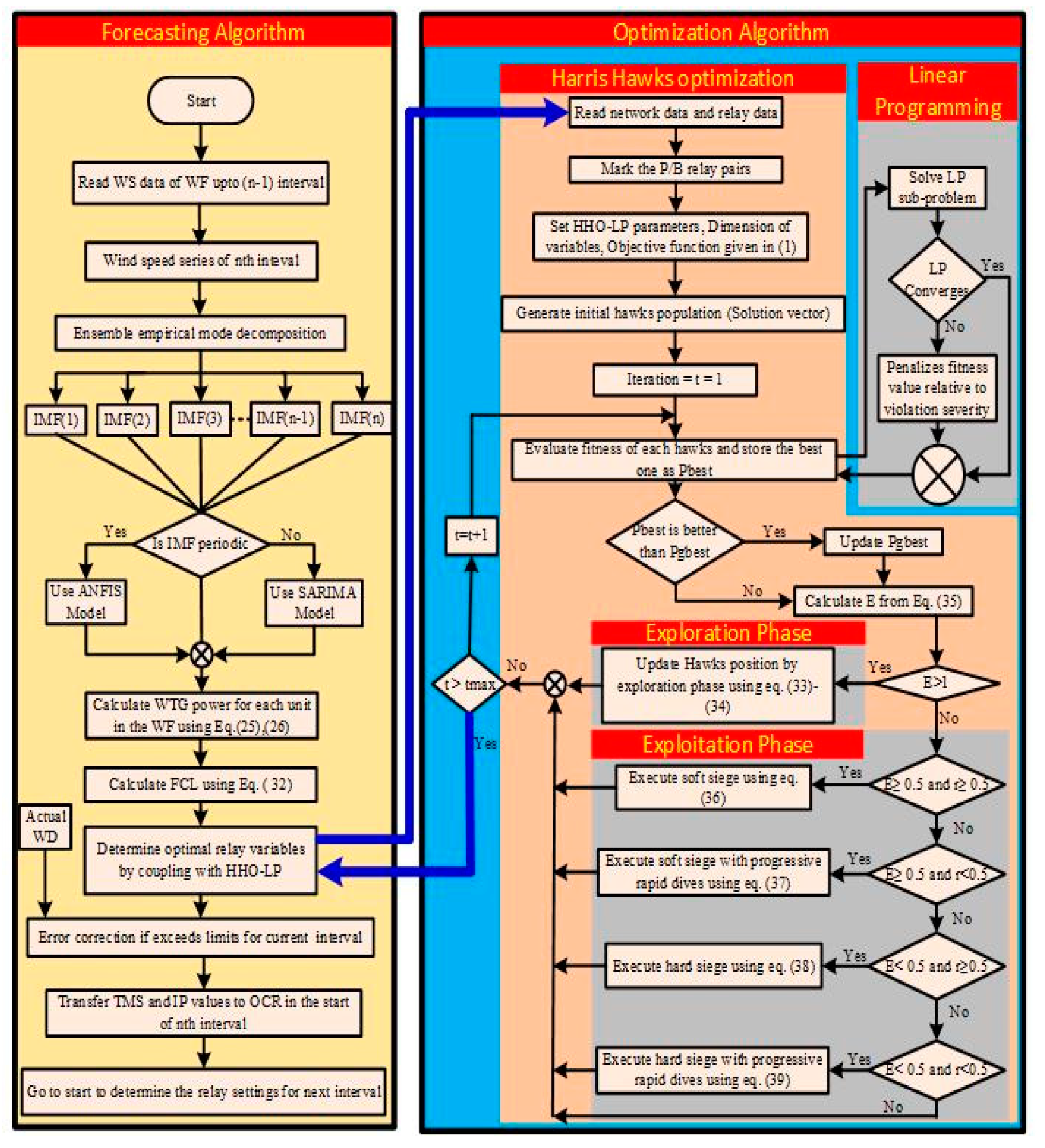
3. Proposed Methodology
3.1. EEMD
- (1)
- Initialize the number of ensembles (M) and the amplitude of the added white noise; set i = 1.
- (2)
- Add a white noise series to the original wind speed series x(t).where ni(t) denotes the i-th added white noise series, and xi(t) denotes the series with the added white noise.
- (3)
- Decompose the series xi(t) into J IMFs cij(t) (j = 1, 2, …, J) using the EMD method, where cij(t) is the j-th IMF after the i-th trial, and J is the number of IMFs.
- (4)
- If i < M, then go to Step (2) with i = i + 1. Repeat Steps (2) and (3) with different white noise series.
- (5)
- Calculate the ensemble mean cj(t) of the M trials for each IMF of the decomposition as the final results.where cj(t), (j = 1, 2, …, J) is the j-th IMF component using the EEMD method.
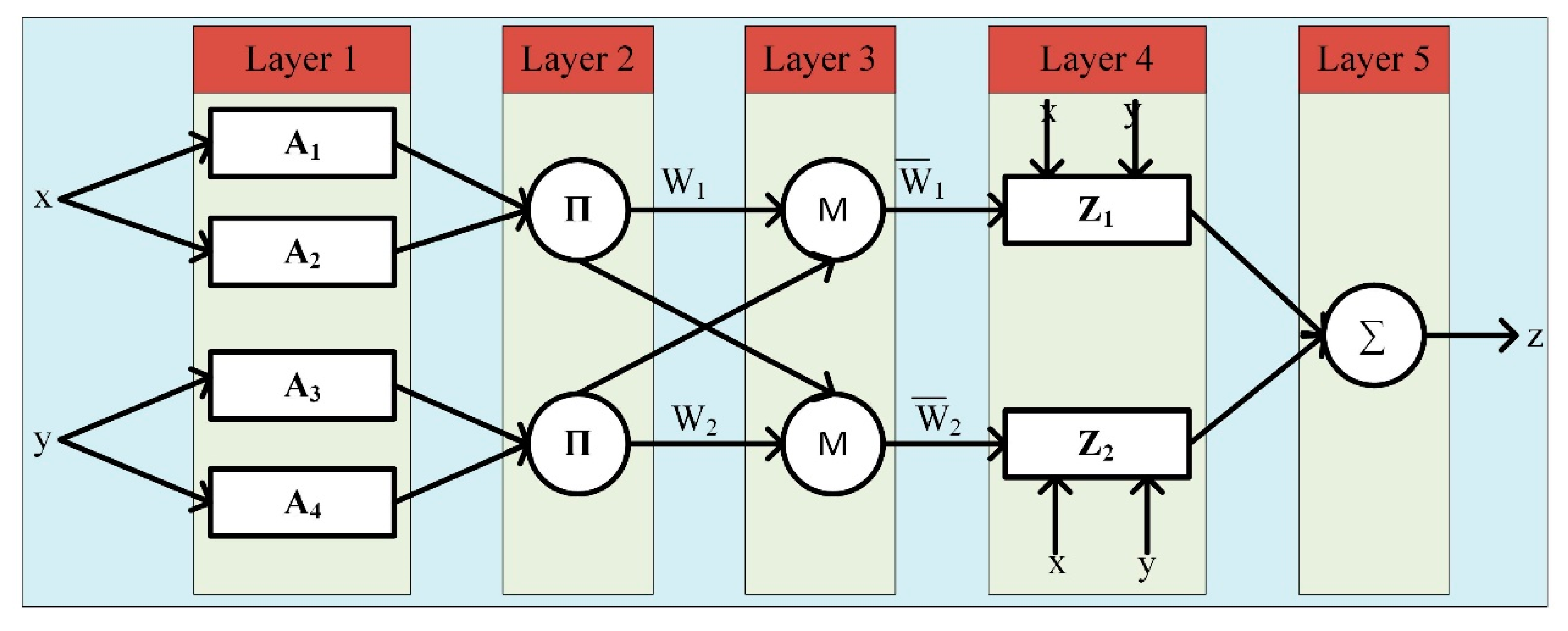
3.2. ANFIS
3.3. SARIMA
3.4. Hybrid ANFIS–SARIMA Model
- (i)
- The WSS is decomposed into IMFs, and one residual series is given aswhere S(t) is the wind speed series, Ii(t) represents the IMFs, and Rn(t) is the residual series.
- (ii)
- The periodic and nonperiodic series of Ii(t) and Rn(t) are defined as Pj(t) and Ni(t), respectively. Thus, the original wind speed series can be given aswhere Ni(t) is the nonperiodic WSS, and Pj(t) is the periodic WSS.
- (iii)
- For Pj(t), the SARIMA model is implemented and the results are defined as j(t), Whereas, for Ni(t) and Rn(t), the ANFIS model is implemented and the results are defined as (t) and (t). The sum of results of ANFIS–SARIMA is the forecasted wind speed given as
- (iv)
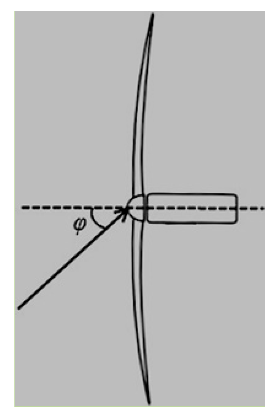
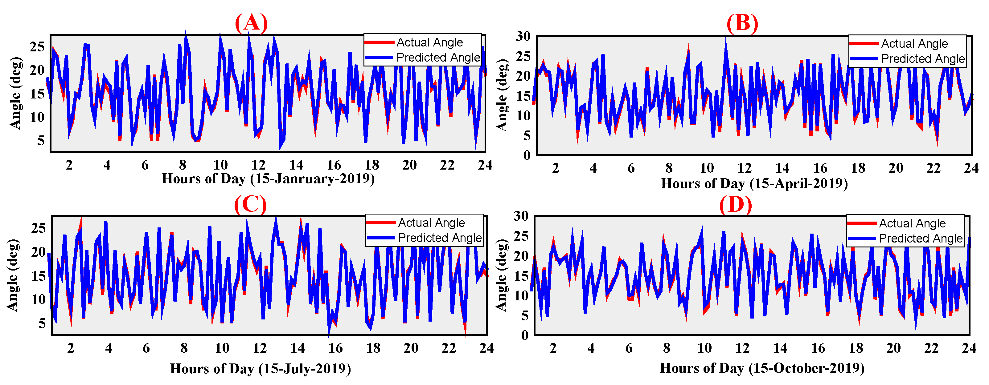
- On the basis of the predicted wind speed in Equation (20), the wind power can be expressed in the form of wind power flux or kinetic energy flux given aswhere ρ(t) is the density of air, P(t) is the atmospheric pressure, Rs is the specific gas density, and T(t) is the atmospheric temperature. A is the rotor swept area, Cp is the coefficient of maximum power, and S(t) is the forecasted wind speed. If the wind hits the turbine at an angle φ(t), as shown in Figure 2, then the azimuthal angle variation in the airflow can be considered as cosφ(t), and Equation (21) can be written as
- (v)
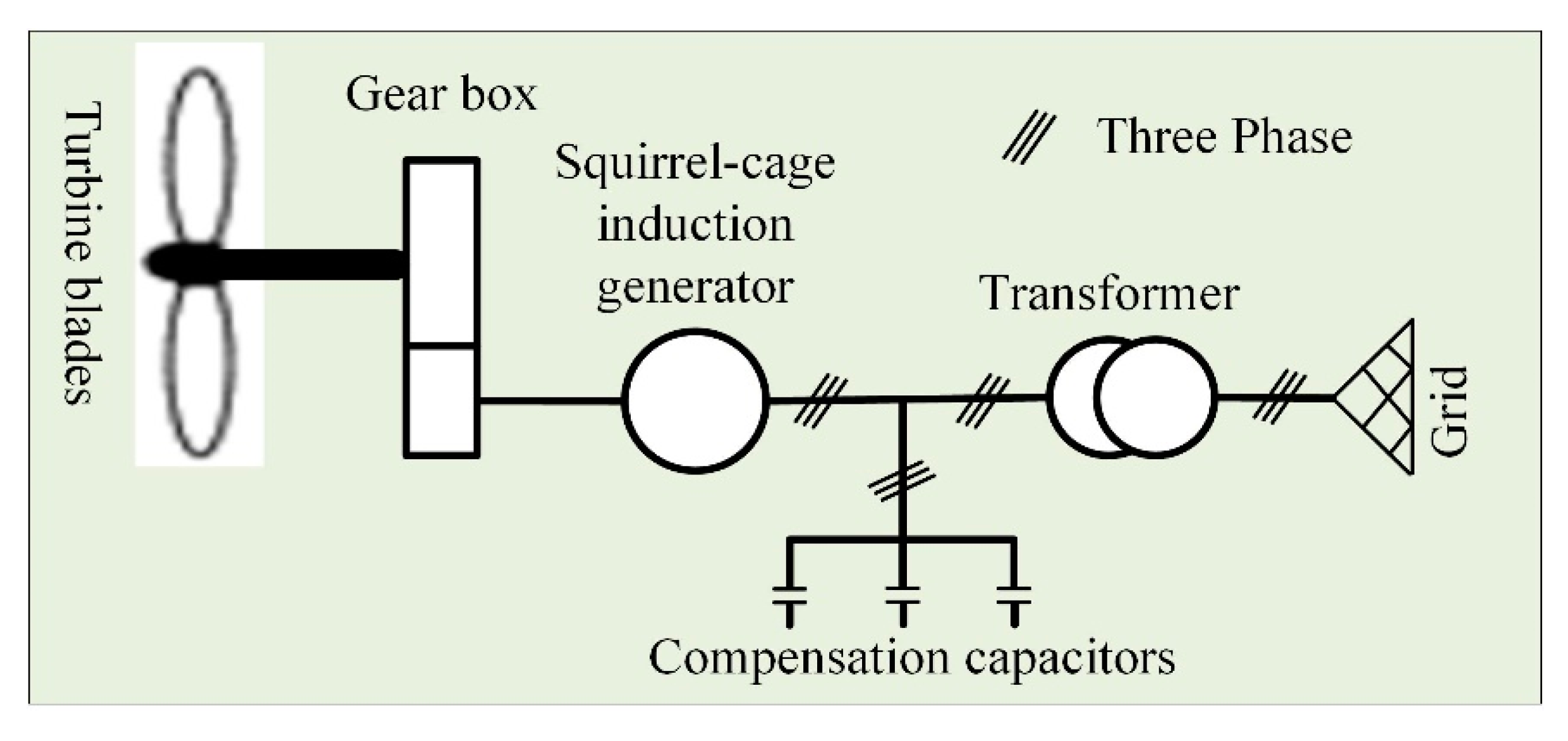
- The squirrel-cage induction generator (SCIG) and doubly fed induction generator (DFIG) are used almost exclusively in the energy conversion stage of the induction generator wind power system. In this study, SCIG was used. The most commonly used system topology is an SCIG directly connected to the power grid, as shown in Figure 3. This topology implies a constant frequency and voltage of the SCIG that establishes a fixed-speed operation. In such a system, the SCIG relies on the grid (or capacitor bank) to provide reactive power, which is necessary to build electromagnetic excitation for the rotary field. The generating mode of the SCIG is triggered by driven torque, which acts opposite to the generator speed within the super-synchronous speed operation region. Due to the absence of a power electronics interface, such a system can only serve the grid support applications, wherein just limited control (pitch-angle control) can be applied.
- (vi)
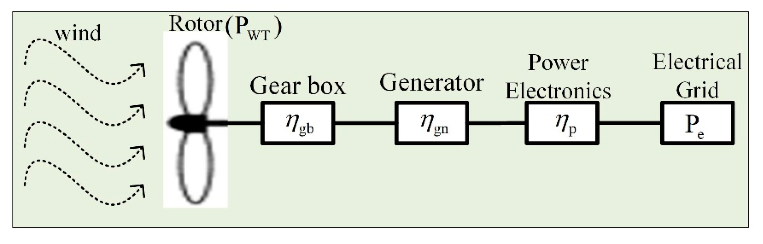
- The electrical power transferred to the grid is given asHere, the efficiency for the gearbox is 0.95, that for the generator is 0.97, and that for the power electronics device is 0.98 [47]. the current from the WTG in the wind farm can be calculated aswhere cos is the power factor, and VL is the line voltage.
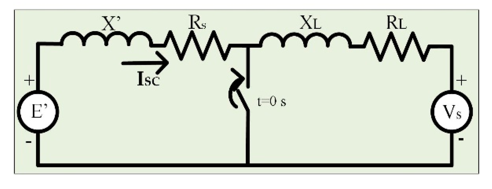
- (vii)
- The fault current from a three-phase fault in a squirrel-cage induction machine is calculated using the network shown in Figure 5 [48]. The short-circuit current value at t = 0 is given aswhere is the voltage behind transient reactance , Rs is the stator resistance, Xs and Xr are the leakage reactance of the stator and rotor, respectively, Xm is the magnetizing reactance, and RL and XL are the resistance and reactance of the line connecting the WTG and grid. Substituting Equation (29) into Equation (28), the short-circuit current for a particular instance can be given asAll the terms in Equation (31) are constant for an SCIG; thus, the fault current depends upon the value of IWTG calculated in Equation (16), which depends upon the wind speed. The total fault current from a wind farm is the sum of fault currents from all the WTGs.
3.5. Hybrid HHO–LP Optimization Algorithm
3.5.1. Harris Hawks Optimization
3.5.2. Linear Programming
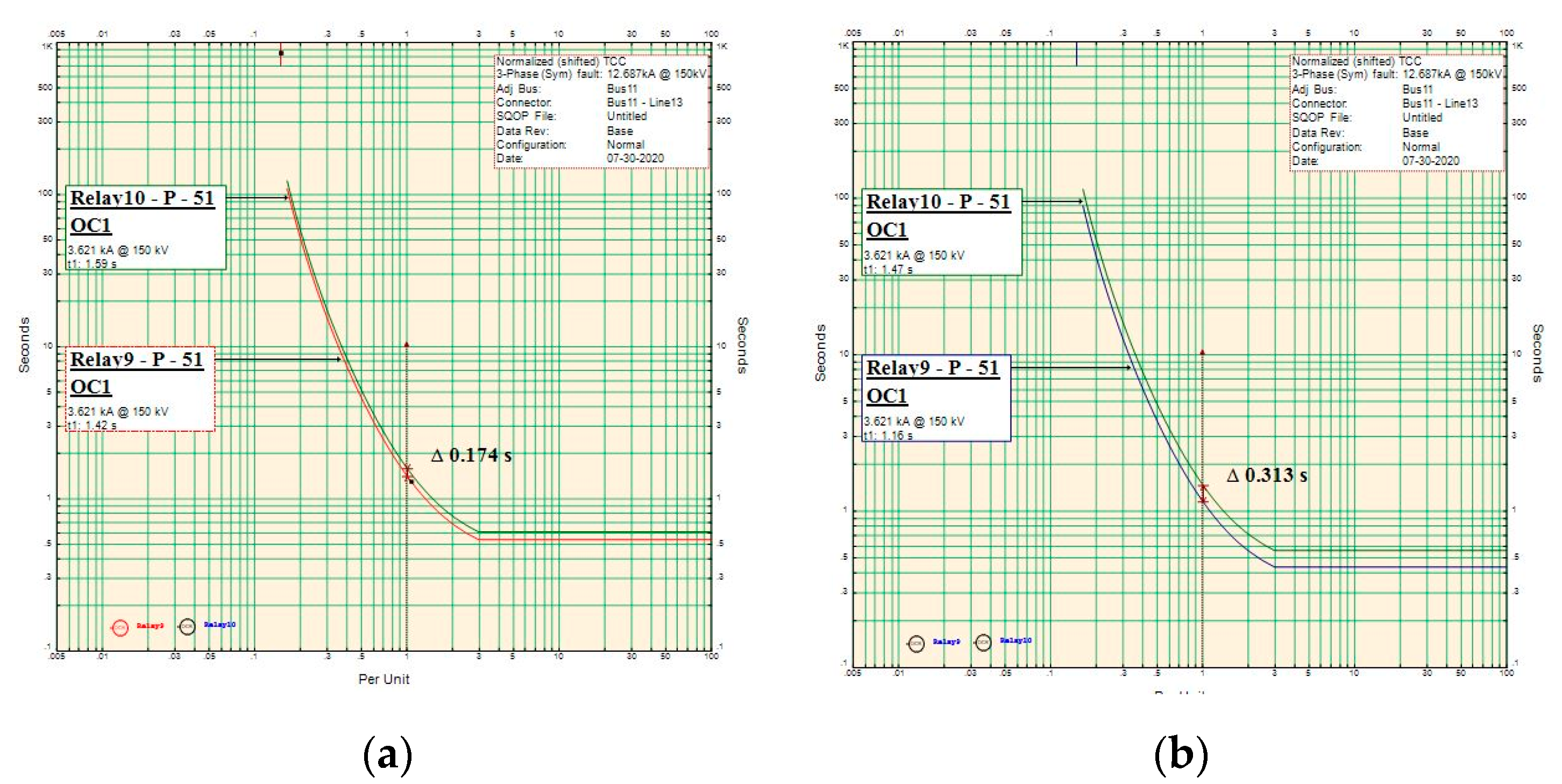
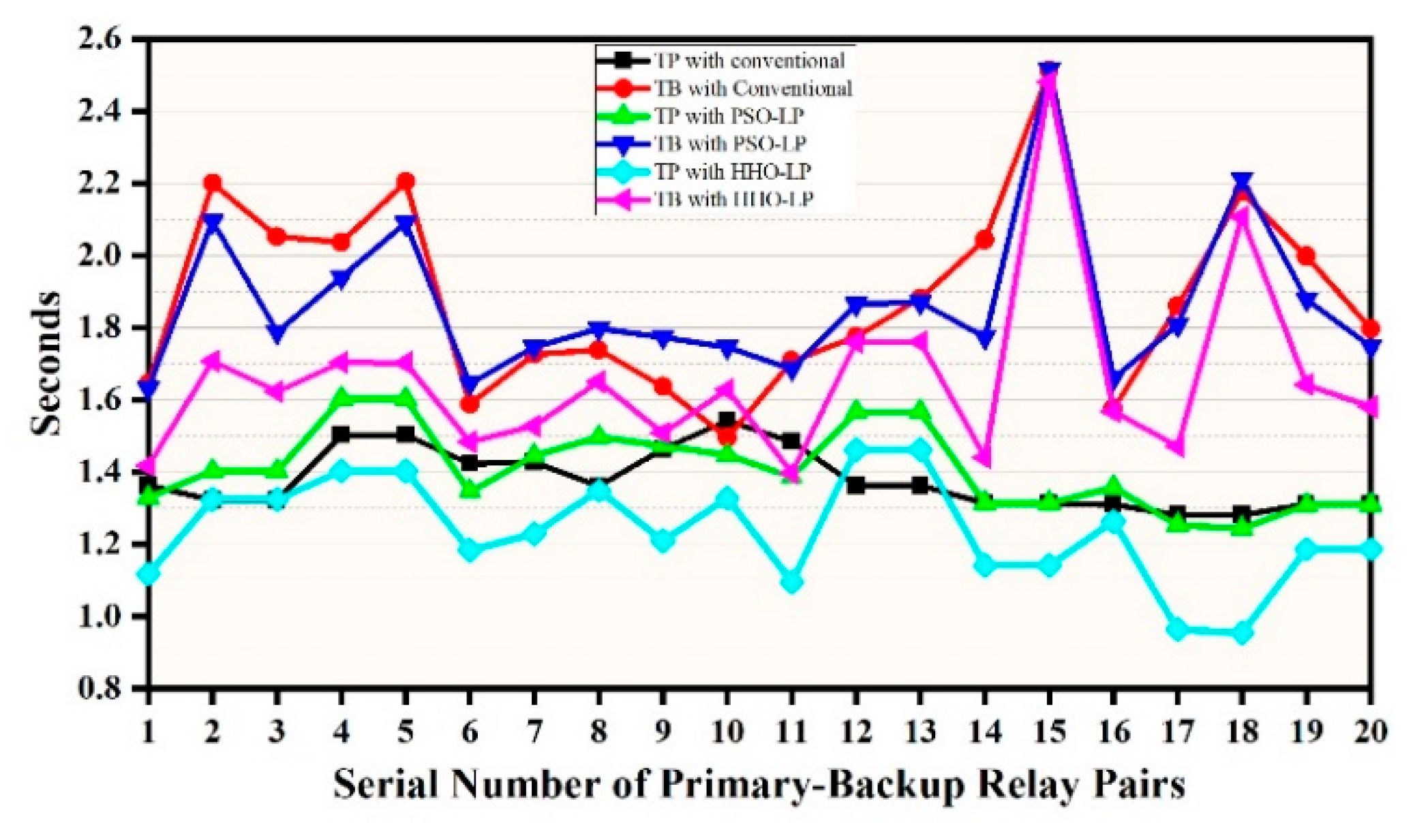
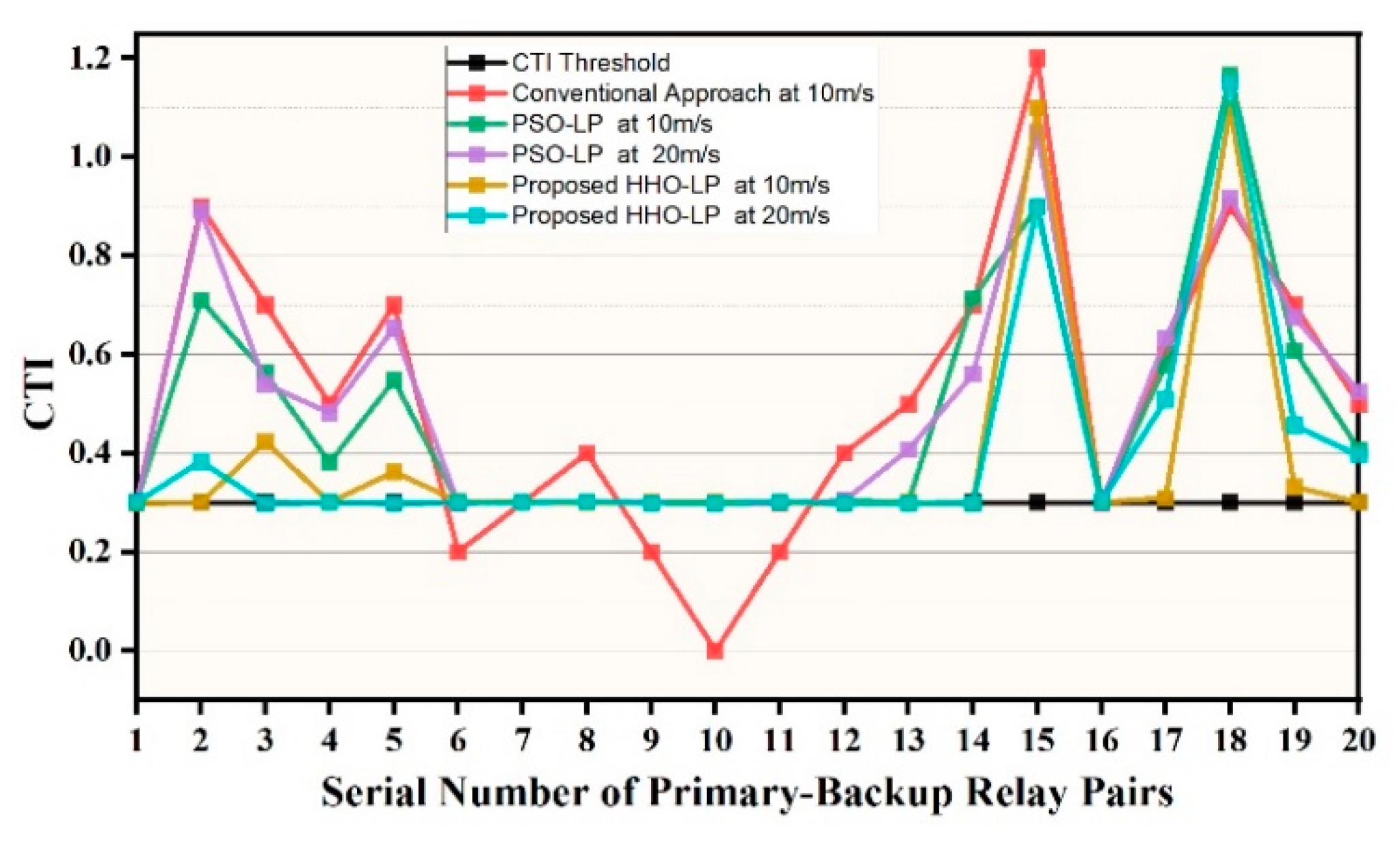
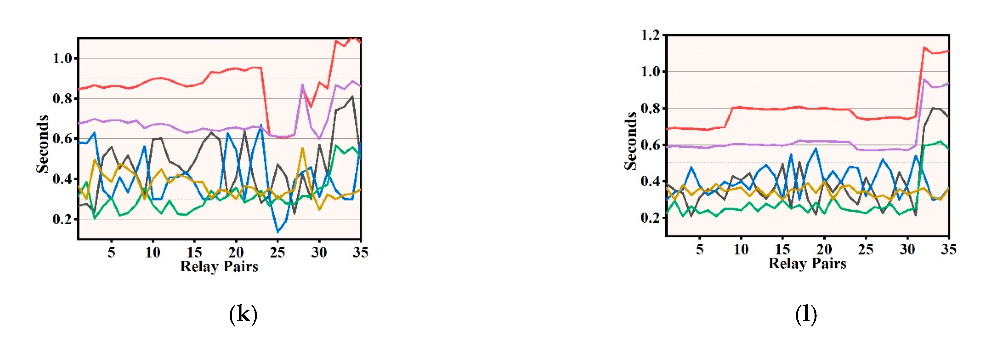
4. Case Studies
4.1. Test System Specification
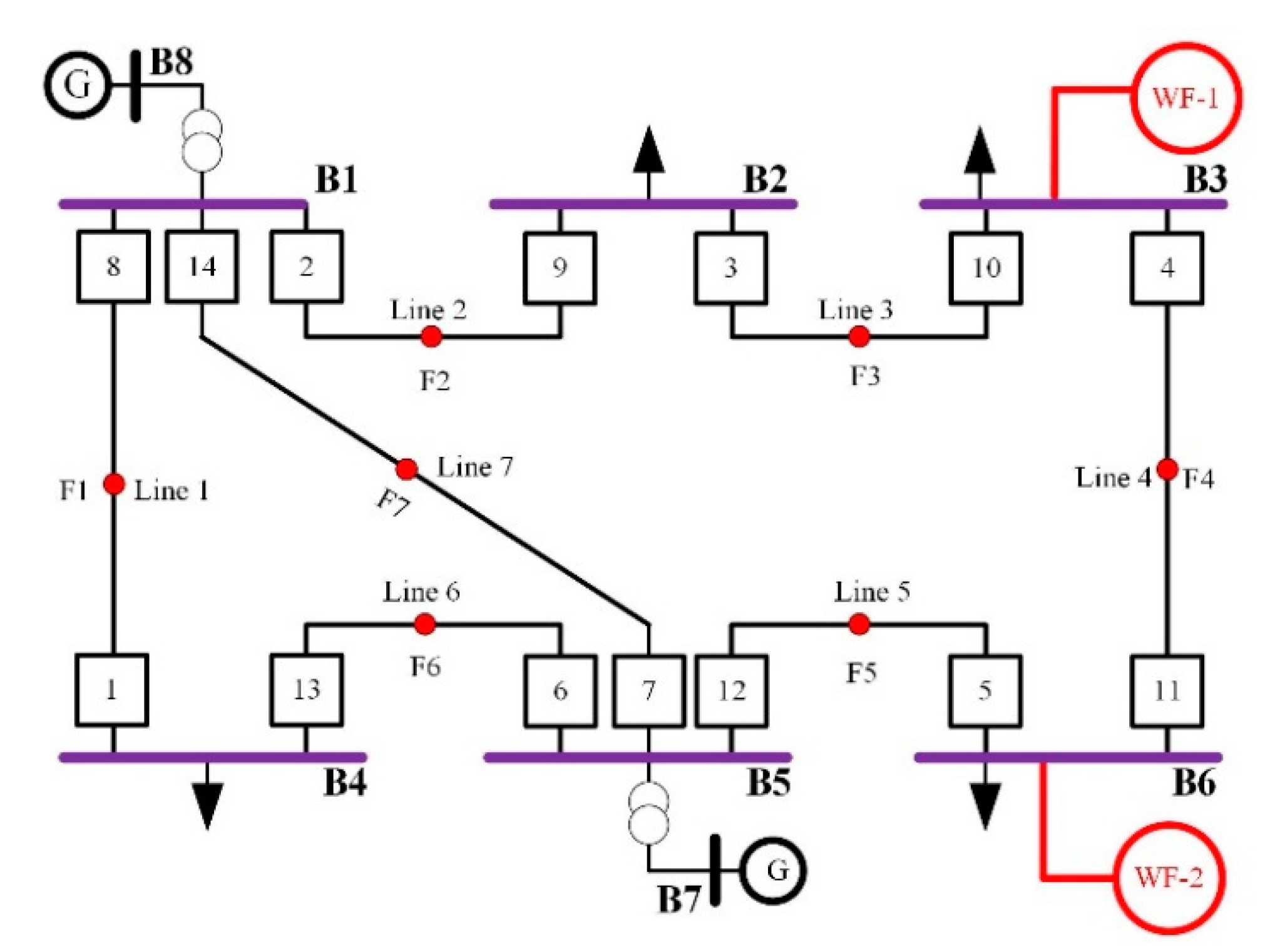
4.1.1. IEEE-8 Bus System
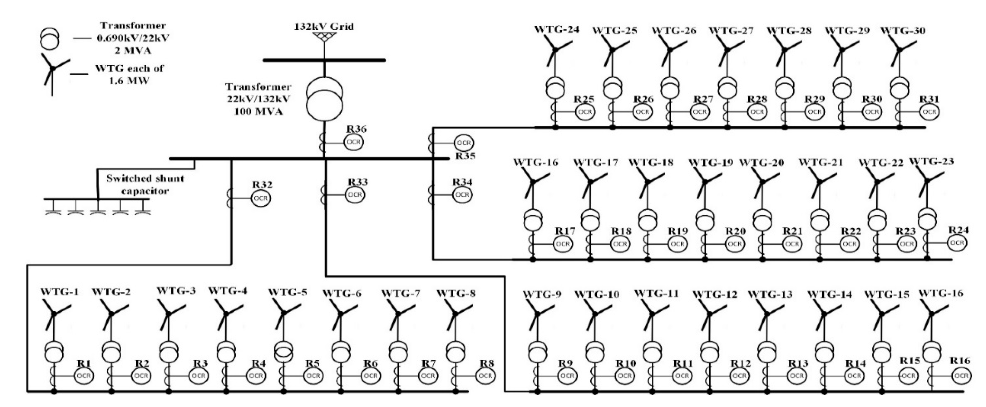
4.1.2. Jhimpir Wind-Farm-Integrated Substation
5. Conclusions
Author Contributions
Funding
Conflicts of Interest
Appendix A

| Parameters | WF-1 | WF-2 | Parameters | WF-1 | WF-2 |
|---|---|---|---|---|---|
| Number of machines | 20 | 10 | Rated wind speed | 13 m/s | |
| Nominal power of each machine | 3 MW | LS | 0.0397 pu | ||
| Generating voltage | 0.690 kV | Lr | 0.0397 pu | ||
| Frequency | 50 Hz | Lm | 1.354 pu | ||
| H(s) | 0.95 | ||||
References
- Guo, X.; Yang, X. The Development of Wind Power under the Low-Carbon Constraints of Thermal Power in the Beijing-Tianjin-Hebei Region. IEEE Access 2020, 8, 44783–44797. [Google Scholar] [CrossRef]
- Zhou, X.; Wang, Z.; Ma, Y.; Gao, Z. An overview on development of wind power generation. In Proceedings of the 2018 IEEE International Conference on Mechatronics and Automation (ICMA), Changchun, China, 5–8 August 2018; pp. 2042–2046. [Google Scholar] [CrossRef]
- Spear, S. Wind Energy Could Generate Nearly 20 Percent of World’s Electricity by 2030. 2014. Available online: https://www.ecowatch.com/wind-energy-could-generate-nearly-20-percent-of-worlds-electricity-by--1881962962.html (accessed on 15 July 2020).
- Dupont, E.; Koppelaar, R.; Jeanmart, H. Global available wind energy with physical and energy return on investment constraints. Appl. Energy 2018, 209, 322–338. [Google Scholar] [CrossRef]
- Dehghanpour, E.; Karegar, H.K.; Kheirollahi, R.; Soleymani, T. Optimal coordination of directional overcurrent relays in microgrids by using cuckoo-linear optimization algorithm and fault current limiter. IEEE Trans. Smart Grid 2018, 9, 1365–1375. [Google Scholar] [CrossRef]
- Purwar, E.; Vishwakarma, D.N.; Singh, S.P. A Novel Constraints Reduction-Based Optimal Relay Coordination Method Considering Variable Operational Status of Distribution System with DGs. IEEE Trans. Smart Grid 2019, 10, 889–898. [Google Scholar] [CrossRef]
- Shamsoddini, M.; Vahidi, B.; Razani, R.; Mohamed, Y.A.R.I. A novel protection scheme for low voltage DC microgrid using inductance estimation. Int. J. Electr. Power Energy Syst. 2020, 120, 105992. [Google Scholar] [CrossRef]
- Farzinfar, M.; Jazaeri, M. A novel methodology in optimal setting of directional fault current limiter and protection of the MG. Int. J. Electr. Power Energy Syst. 2020, 116, 105564. [Google Scholar] [CrossRef]
- Gashteroodkhani, O.A.; Majidi, M.; Etezadi-Amoli, M. A combined deep belief network and time-time transform based intelligent protection Scheme for microgrids. Electr. Power Syst. Res. 2020, 182, 106239. [Google Scholar] [CrossRef]
- El-Naily, N.; Saad, S.M.; Hussein, T.; Mohamed, F.A. A novel constraint and non-standard characteristics for optimal over-current relays coordination to enhance microgrid protection scheme. IET Gener. Transm. Distrib. 2019, 13, 780–793. [Google Scholar] [CrossRef]
- Purwar, E.; Singh, S.P.; Vishwakarma, D.N. A Robust Protection Scheme Based on Hybrid Pick-Up and Optimal Hierarchy Selection of Relays in the Variable DGs-Distribution System. IEEE Trans. Power Deliv. 2020, 35, 150–159. [Google Scholar] [CrossRef]
- Lwin, M.; Guo, J.; Dimitrov, N.B.; Santoso, S. Stochastic Optimization for Discrete Overcurrent Relay Tripping Characteristics and Coordination. IEEE Trans. Smart Grid 2019, 10, 732–740. [Google Scholar] [CrossRef]
- Dubey, R.K.; Samantaray, S.R.; Panigrahi, B.K. Adaptive distance relaying scheme for transmission network connecting wind farms. Electr. Power Compon. Syst. 2014, 42, 1181–1193. [Google Scholar] [CrossRef]
- Ikegami, T.; Urabe, C.T.; Saitou, T.; Ogimoto, K. Numerical definitions of wind power output fluctuations for power system operations. Renew. Energy 2018, 115, 6–15. [Google Scholar] [CrossRef]
- Abdelaziz, A.Y.; Talaat, H.E.A.; Nosseir, A.I.; Hajjar, A.A. An adaptive protection scheme for optimal coordination of overcurrent relays. Electr. Power Syst. Res. 2002, 61, 1–9. [Google Scholar] [CrossRef]
- Rizwan, M.; Hong, L.; Waseem, M.; Shu, W. Sustainable protection coordination in presence of distributed generation with distributed network. Int Trans Electr Energ Syst. 2019, e12217. [Google Scholar] [CrossRef]
- Laway, H.O.; Gupta, A.N. Integrated software for optimal directional overcurrent relay coordination. Electr. Mach. Power Syst. 1994, 22, 125–136. [Google Scholar] [CrossRef]
- Damborg, M.J.; Ramaswami, R.; Venkata, S.S. Group Puget. Computer aided transmission protection system design. IEEE Trans. Power Appar. Syst. 1984, PAS-103, 51–59. [Google Scholar] [CrossRef]
- Sharifian, H.; Abyaneh, H.A.; Salman, S.K.; Mohammadi, R.; Razavi, F. Determination of the minimum break point set using expert system and genetic algorithm. IEEE Trans. Power Deliv. 2010, 25, 1284–1295. [Google Scholar] [CrossRef]
- Ezzeddine, M.; Kaczmarek, R.; Iftikhar, M.U. Coordination of directional overcurrent relays using a novel method to select their settings. IET Gener. Transm. Distrib. 2011, 5, 743–750. [Google Scholar] [CrossRef]
- Razavi, F.; Abyaneh, H.A.; Al-Dabbagh, M.; Mohammadi, R.; Torkaman, H. A new comprehensive genetic algorithm method for optimal overcurrent relays coordination. Electr. Power Syst. Res. 2008, 78, 713–720. [Google Scholar] [CrossRef]
- Chattopadhyay, B. An online relay coordination algorithm for adaptive protection using linear programming technique. IEEE Power Eng. Rev. 1996, 16, 47–48. [Google Scholar]
- Urdaneta, A.J. Coordination of directional overcurrent relay timing using linear programming. IEEE Power Eng. Rev. 1996, 16, 44–45. [Google Scholar] [CrossRef]
- Roy, S.; Babu, P.S.; Babu, N.V.P. Intelligent Overcurrent and Distance Relays Coordination: A Comparative Analysis using GA, PSO and TLBO. In Proceedings of the 2018 4th International Conference on Electrical Energy Systems (ICEES), Chennai, India, 7–9 February 2018; pp. 162–167. [Google Scholar] [CrossRef]
- Zeineldin, H.H.; El-Saadany, E.F.; Salama, M.M.A. Optimal coordination of overcurrent relays using a modified particle swarm optimization. Electr. Power Syst. Res. 2006, 76, 988–995. [Google Scholar] [CrossRef]
- Amraee, T. Coordination of Directional Overcurrent. IEEE Trans. Power Deliv. 2012, 27, 1415–1422. [Google Scholar] [CrossRef]
- Bedekar, P.P.; Bhide, S.R. Optimum coordination of overcurrent relay timing using continuous genetic algorithm. Expert Syst. Appl. 2011, 38, 11286–11292. [Google Scholar] [CrossRef]
- Orazgaliyev, D.; Tleubayev, A.; Zholdaskhan, B.; Nunna, H.S.V.S.K.; Dadlani, A.; Doolla, S. Adaptive Coordination Mechanism of Overcurrent Relays using Evolutionary Optimization Algorithms for Distribution Systems with DGs. In Proceedings of the 2019 International Conference on Smart Energy Systems and Technologies (SEST), IPorto, Portugal, 9–11 September 2019; pp. 1–6. [Google Scholar] [CrossRef]
- Singh, M.; Panigrahi, B.K.; Abhyankar, A.R. Optimal coordination of directional over-current relays using Teaching Learning-Based Optimization (TLBO) algorithm. Int. J. Electr. Power Energy Syst. 2013, 50, 33–41. [Google Scholar] [CrossRef]
- Tripathi, J.M.; Adhishree, S.; Krishan, R. Optimal coordination of overcurrent relays using gravitational search algorithm with DG penetration. In Proceedings of the 2014 6th IEEE Power India International Conference (PIICON), Delhi, India, 5–7 December 2014; pp. 1–6. [Google Scholar] [CrossRef]
- Saha, D.; Datta, A.; Das, P. Optimal coordination of directional overcurrent relays in power systems using symbiotic organism search optimisation technique. IET Gener. Transm. Distrib. 2016, 10, 2681–2688. [Google Scholar] [CrossRef]
- ARivas, E.L.; Pareja, L.A.G.; Abrão, T. Coordination of distance and directional overcurrent relays using an extended continuous domain ACO algorithm and an hybrid ACO algorithm. Electr. Power Syst. Res. 2019, 170, 259–272. [Google Scholar] [CrossRef]
- Moradi, M.H.; Abedinie, M. A combination of genetic algorithm and particle swarm optimization for optimal DG location and sizing in distribution systems. In Proceedings of the 2010 9th Internation Power Energy Conference IPEC, Singapore, 27–29 October 2010; pp. 858–862. [Google Scholar] [CrossRef]
- Sanjay, R.; Jayabarathi, T.; Raghunathan, T.; Ramesh, V.; Mithulananthan, N. Optimal allocation of distributed generation using hybrid grey Wolf optimizer. IEEE Access 2017, 5, 14807–14818. [Google Scholar] [CrossRef]
- Darabi, A.; Bagheri, M.; Gharehpetian, G.B. Electrical Power and Energy Systems metaheuristic approaches for exact overcurrent relay coordination. Int. J. Electr. Power Energy Syst. 2020, 114, 105420. [Google Scholar] [CrossRef]
- Srinivas, S.T.P.; Swarup, K.S. Optimal Relay Coordination for Microgrids Using Hybrid Modified Particle Swarm Optimization–Interval Linear Programming Approach. In Proceedings of the 2017 North American Power Symposium (NAPS), Morgantown, WV, USA, 17–19 September 2017. [Google Scholar]
- Kale, V.S.; Agarwal, M.; Kesarkar, P.D.; Regmi, D.R.; Chaudhary, A.; Killawala, C. Optimal coordination of overcurrent relays using genetic algorithm and simulated annealing. In Proceedings of the 2014 International Conference on Control, Instrumentation, Energy and Communication (CIEC), Calcutta, India, 31 January–2 February 2014; pp. 361–365. [Google Scholar] [CrossRef]
- Al-Roomi, A.R.; El-Hawary, M.E. Optimal coordination of double primary directional overcurrent relays using a new combinational bbo/de algorithm. Can. J. Electr. Comput. Eng. 2019, 42, 135–147. [Google Scholar] [CrossRef]
- Noghabi, A.S.; Sadeh, J.; Mashhadi, H.R. Considering different network topologies in optimal overcurrent relay coordination using a hybrid GA. IEEE Trans. Power Deliv. 2009, 24, 1857–1863. [Google Scholar] [CrossRef]
- Wagner, R.; Antoniou, I.; Pedersen, S.M.; Courtney, M.S.; Jørgensen, H.E. The influence of the wind speed profile on wind turbine performance measurements. Wind Energy 2009, 12, 348–362. [Google Scholar] [CrossRef]
- Kuo, C.; Lin, W.S.; Dressel, C.a.; Chiu, A.W.L. Ensemble Empirical Mode Decomposition. Source 2011, 55, 6281–6284. [Google Scholar]
- Geurts, M.; Box, G.E.P.; Jenkins, G.M. Time Series Analysis: Forecasting and Control. J. Mark. Res. 1977, 14, 269. [Google Scholar] [CrossRef]
- Zhang, J.; Wei, Y.M.; Tan, Z.F.; Wang, K.; Tian, W. A hybrid method for short-term wind speed forecasting. Sustainability 2017, 9, 596. [Google Scholar] [CrossRef]
- Khosravi, A.; Koury, R.N.N.; Machado, L.; Pabon, J.J.G. Prediction of wind speed and wind direction using artificial neural network, support vector regression and adaptive neuro-fuzzy inference system. Sustain. Energy Technol. Assess. 2018, 25, 146–160. [Google Scholar] [CrossRef]
- Reynolds, O.; April, R., IV. On the dynamical theory of incompressible viscous fluids and the determination of the criterion. Philos. Trans. R. Soc. Lond. 1895, 186, 123–164. [Google Scholar] [CrossRef]
- Choukulkar, A.; Pichugina, Y.; Clack, C.T.M.; Calhoun, R.; Banta, R.; Brewer, A.; Hardesty, M. A new formulation for rotor equivalent wind speed for wind resource assessment and wind power forecasting. Wind Energy 2016, 19, 1439–1452. [Google Scholar] [CrossRef]
- Baskut, O.; Ozgener, O.; Ozgener, L. Effects of meteorological variables on exergetic efficiency of wind turbine power plants. Renew. Sustain. Energy Rev. 2010, 14, 3237–3241. [Google Scholar] [CrossRef]
- Ojaghi, M.; Mohammadi, M. Unified modeling technique for axially uniform and nonuniform eccentricity faults in three-phase squirrel cage induction motors. IEEE Trans. Ind. Electr. 2018, 65, 5292–5301. [Google Scholar] [CrossRef]
- Heidari, A.A.; Mirjalili, S.; Faris, H.; Aljarah, I.; Mafarja, M.; Chen, H. Harris hawks optimization: Algorithm and applications. Futur. Gener. Comput. Syst. 2019, 97, 849–872. [Google Scholar] [CrossRef]
- Zhou, J.; Shi, J.; Li, G. Fine tuning support vector machines for short-term wind speed forecasting. Energy Convers. Manag. 2011, 52, 1990–1998. [Google Scholar] [CrossRef]
- Nguyen, L.; Metzger, M. Comparison of forecasting methods for vertical axis wind turbine applications in an urban/suburban area. J. Renew. Sustain. Energy 2017, 9. [Google Scholar] [CrossRef]
- Hong, Y.Y.; Rioflorido, C.L.P.P. A hybrid deep learning-based neural network for 24-h ahead wind power forecasting. Appl. Energy 2019, 250, 530–539. [Google Scholar] [CrossRef]
- Luo, X.; Sun, J.; Wang, L.; Wang, W.; Zhao, W.; Wu, J.; Wang, J.-H.; Zhang, Z. Short-term wind speed forecasting via stacked extreme learning machine with generalized correntropy. IEEE Trans. Ind. Inform. 2018, 14, 4963–4971. [Google Scholar] [CrossRef]
- Chabanloo, R.M.; Abyaneh, H.A.; Kamangar, S.S.H.; Razavi, F. Optimal combined overcurrent and distance relays coordination incorporating intelligent overcurrent relays characteristic selection. IEEE Trans. Power Deliv. 2011, 26, 1381–1391. [Google Scholar] [CrossRef]
- Papaspiliotopoulos, V.A.; Kurashvili, T.A.; Korres, G.N. Optimal coordination of directional overcurrent relays in distribution systems with distributed generation based on a hybrid PSO-LP algorithm. IET Conf. Publ. 2014, 2014, 1–6. [Google Scholar] [CrossRef]
- Pakistan’s Alternative Energy Development Board. Available online: http://www.aedb.org/ (accessed on 15 July 2020).


| No | Strategies | Escape Energy (E) | Escape Probability (r) |
|---|---|---|---|
| 1 | Soft siege (SS) | E ≥ 0.5 | r ≥ 0.5 |
| 2 | Soft siege with progressive rapid dives (SSPRD) | E ≥ 0.5 | r < 0.5 |
| 3 | Hard siege (HS) | E < 0.5 | r ≥ 0.5 |
| 4 | Hard siege with progressive rapid dives (HSPRD) | E < 0.5 | r < 0.5 |
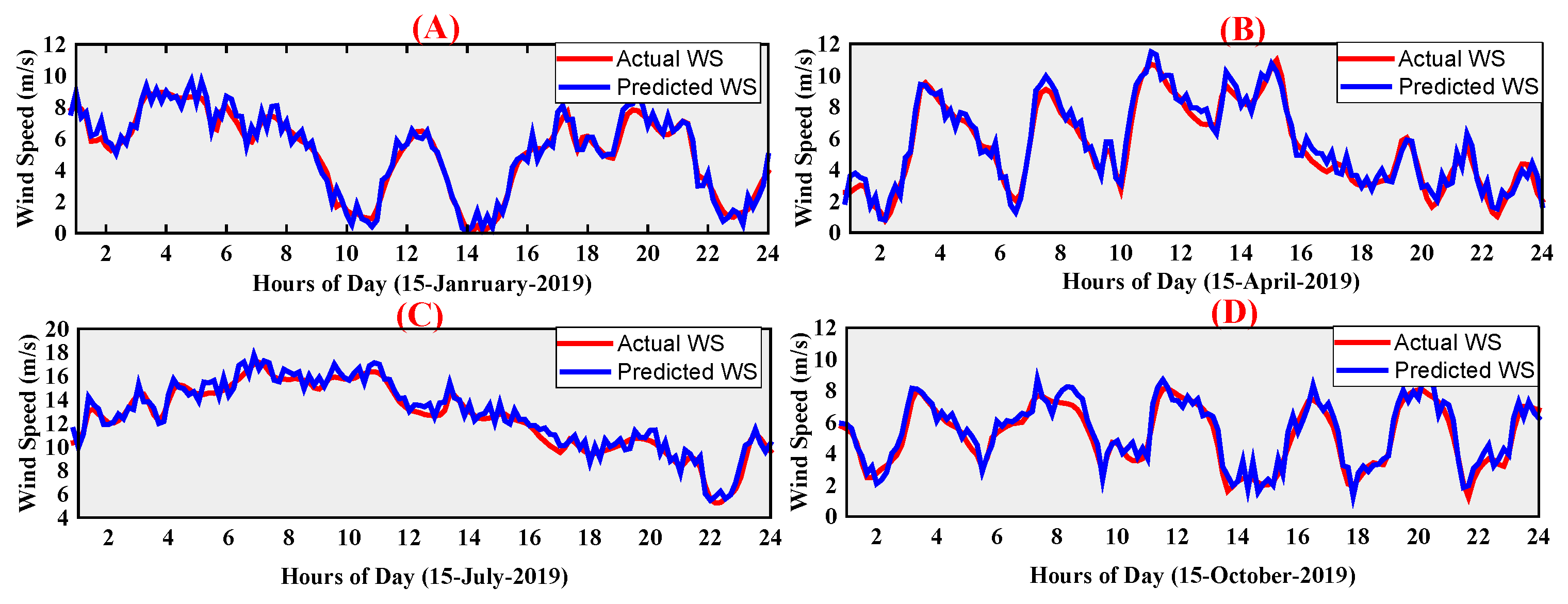
| Errors | FTSVM [50] | MPM [51] | CNN–RBFNN [52] | SELM [53] | Hybrid ANFIS–SARIMA |
|---|---|---|---|---|---|
| ME | 0.0947 | 0.0850 | 0.0764 | 0.0658 | 0.0625 |
| MAE | 1.3412 | 1.3210 | 1.3072 | 1.1064 | 0.9643 |
| MSE | 16.512 | 15.5413 | 13.7651 | 11.5614 | 11.0312 |
| RMSE | 3.2314 | 3.1150 | 2.8574 | 2.4358 | 2.3519 |
| ESD | 4.6864 | 4.5754 | 4.1523 | 3.9525 | 3.8798 |
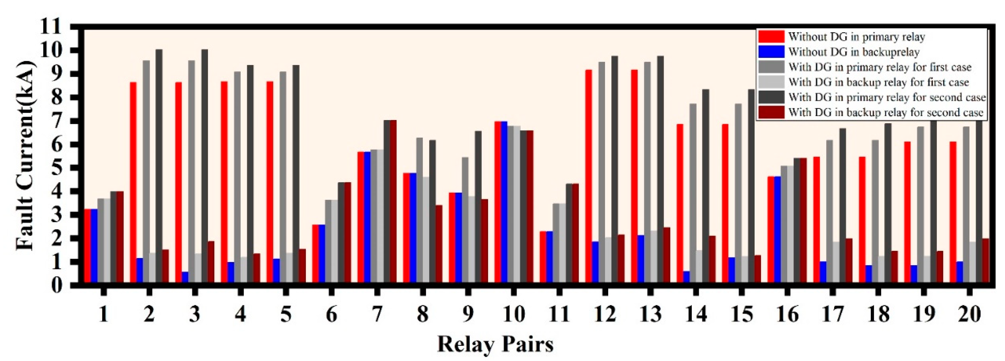
| Fault | Pair | PR | BR | Fault | Pair | PR | BR | Fault | Pair | PR | BR |
|---|---|---|---|---|---|---|---|---|---|---|---|
| F1 | 1 | 1 | 6 | F3 | 7 | 3 | 2 | F6 | 14 | 6 | 5 |
| 2 | 8 | 7 | 8 | 10 | 11 | 15 | 6 | 14 | |||
| 3 | 8 | 9 | F4 | 9 | 4 | 3 | 16 | 13 | 8 | ||
| F2 | 4 | 2 | 1 | 10 | 11 | 12 | F7 | 17 | 7 | 5 | |
| 5 | 2 | 7 | F5 | 11 | 5 | 4 | 18 | 7 | 13 | ||
| 6 | 9 | 10 | 12 | 12 | 13 | 19 | 14 | 1 | |||
| 13 | 12 | 14 | 20 | 14 | 9 |
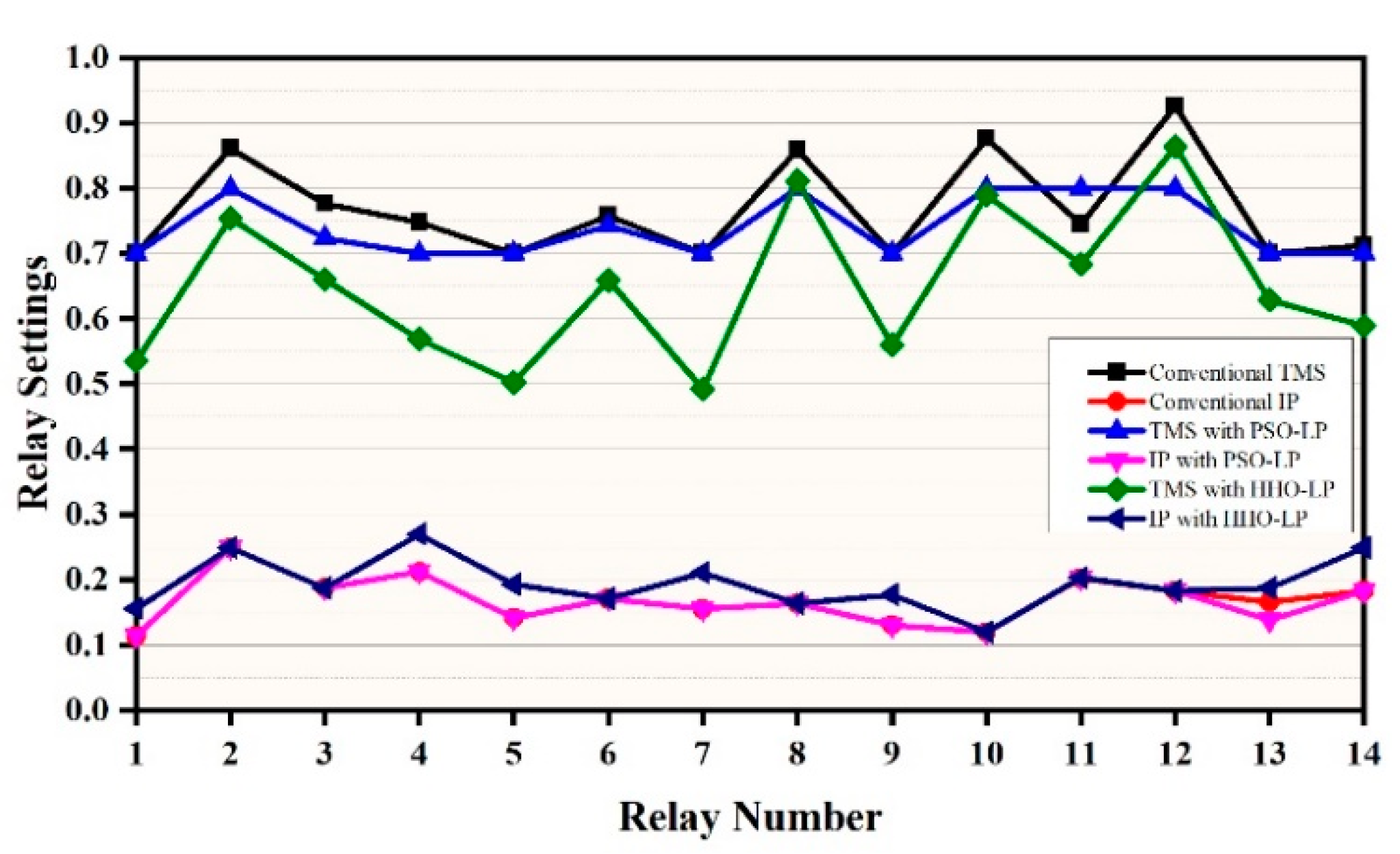
| Relay | Conventional | PSO–LP [55] | HHO–LP | |||
|---|---|---|---|---|---|---|
| TMS | Ip (kA) | TMS | Ip (kA) | TMS | Ip (kA) | |
| 1 | 0.7 | 0.114 | 0.6 | 0.124 | 0.471 | 0.156 |
| 2 | 0.8 | 0.249 | 0.806 | 0.249 | 0.685 | 0.249 |
| 3 | 0.724 | 0.187 | 0.729 | 0.187 | 0.597 | 0.187 |
| 4 | 0.7 | 0.213 | 0.648 | 0.21 | 0.464 | 0.27 |
| 5 | 0.7 | 0.142 | 0.6 | 0.142 | 0.399 | 0.193 |
| 6 | 0.743 | 0.171 | 0.677 | 0.171 | 0.592 | 0.171 |
| 7 | 0.7 | 0.155 | 0.6 | 0.155 | 0.448 | 0.211 |
| 8 | 0.8 | 0.164 | 0.827 | 0.164 | 0.815 | 0.163 |
| 9 | 0.7 | 0.13 | 0.6 | 0.131 | 0.522 | 0.177 |
| 10 | 0.8 | 0.12 | 0.767 | 0.12 | 0.742 | 0.121 |
| 11 | 0.8 | 0.203 | 0.731 | 0.203 | 0.712 | 0.202 |
| 12 | 0.8 | 0.183 | 0.913 | 0.183 | 0.894 | 0.183 |
| 13 | 0.7 | 0.138 | 0.647 | 0.187 | 0.635 | 0.187 |
| 14 | 0.7 | 0.183 | 0.605 | 0.249 | 0.594 | 0.249 |
| Pair | PR | BR | Conventional | PSO–LP [55] | HHO–LP | |||
|---|---|---|---|---|---|---|---|---|
| TOPPR | TOPBR | TOPPR | TOPBR | TOPPR | TOPBR | |||
| 1 | 1 | 6 | 1.362 | 1.643 | 1.197 | 1.497 | 1.010 | 1.309 |
| 2 | 8 | 7 | 1.322 | 2.199 | 1.367 | 1.885 | 1.345 | 1.645 |
| 3 | 8 | 9 | 1.322 | 2.051 | 1.367 | 1.764 | 1.345 | 1.768 |
| 4 | 2 | 1 | 1.502 | 2.036 | 1.513 | 1.812 | 1.286 | 1.586 |
| 5 | 2 | 7 | 1.502 | 2.203 | 1.513 | 1.888 | 1.286 | 1.648 |
| 6 | 9 | 10 | 1.424 | 1.588 | 1.223 | 1.522 | 1.174 | 1.476 |
| 7 | 3 | 2 | 1.427 | 1.725 | 1.437 | 1.738 | 1.177 | 1.477 |
| 8 | 10 | 11 | 1.360 | 1.738 | 1.304 | 1.588 | 1.264 | 1.544 |
| 9 | 4 | 3 | 1.463 | 1.636 | 1.348 | 1.647 | 1.049 | 1.349 |
| 10 | 11 | 12 | 1.541 | 1.495 | 1.408 | 1.706 | 1.369 | 1.671 |
| 11 | 5 | 4 | 1.484 | 1.707 | 1.272 | 1.572 | 0.939 | 1.240 |
| 12 | 12 | 13 | 1.362 | 1.774 | 1.555 | 1.855 | 1.523 | 1.820 |
| 13 | 12 | 14 | 1.362 | 1.881 | 1.555 | 1.856 | 1.523 | 1.822 |
| 14 | 6 | 5 | 1.314 | 2.043 | 1.197 | 1.751 | 1.047 | 1.344 |
| 15 | 6 | 14 | 1.314 | 2.512 | 1.197 | 2.595 | 1.047 | 2.548 |
| 16 | 13 | 8 | 1.310 | 1.577 | 1.326 | 1.628 | 1.302 | 1.602 |
| 17 | 7 | 5 | 1.281 | 1.860 | 1.098 | 1.594 | 0.897 | 1.207 |
| 18 | 7 | 13 | 1.281 | 2.174 | 1.098 | 2.338 | 0.897 | 2.295 |
| 19 | 14 | 1 | 1.310 | 1.997 | 1.242 | 1.776 | 1.220 | 1.551 |
| 20 | 14 | 9 | 1.310 | 1.796 | 1.242 | 1.544 | 1.220 | 1.520 |
| WTG Size and Location | PSO–LP [55] | HHO–LP | ||
|---|---|---|---|---|
| TOPPR | TOPBR | TOPPR | TOPBR | |
| 20 WTGs of 1.5 MVA each at bus 3 | 17.17 s | 23.85 s | 15.88 s | 21.36 s |
| 15 WTGs of 2.5 MVA each at bus 4 | 15.25 s | 22.44 s | 13.44 s | 19.57 s |
| 20 WTGs at bus 3 and 10 WTGs at bus 4 each of 1.5 MVA | 28.17 s | 37.27 s | 24.73 s | 33.16 s |
| 15 WTGs at bus 3 and 10 WTGs at bus 6 each of 1.5 MVA | 26.47 s | 35.57 s | 23.93 s | 32.43 s |
| WTG Integration | Conventional Settings | PSO–LP [55] | Proposed Approach HHO–LP | |||
|---|---|---|---|---|---|---|
| Bus No. | Size (MW) | Operation Time (s) | Operation Time (s) | Time Reduction (%) | Operation Time (s) | Time Reduction (%) |
| 3 | 30 | 52.14 | 41.02 | 21.327 | 37.24 | 28.577 |
| 4 | 37.5 | 48.76 | 37.69 | 22.703 | 33.01 | 32.301 |
| 3, 6 | 60, 30 | 72.28 | 62.038 | 14.169 | 56.36 | 22.026 |
| 3, 4 | 30, 15 | 76.06 | 65.44 | 13.963 | 57.89 | 23.889 |
| 3, 6 | 22.5, 15 | 75.44 | 62.04 | 17.623 | 56.36 | 25.292 |
| Pair | PR | BR1 | BR2 | Pair | PR | BR1 | BR2 | Pair | PR | BR1 | BR2 | Pair | PR | BR1 | BR2 |
|---|---|---|---|---|---|---|---|---|---|---|---|---|---|---|---|
| 1 | R1 | R32 | R36 | 10 | R10 | R33 | R36 | 19 | R19 | R34 | R36 | 28 | R28 | R35 | R36 |
| 2 | R2 | R32 | R36 | 11 | R11 | R33 | R36 | 20 | R20 | R34 | R36 | 29 | R29 | R35 | R36 |
| 3 | R3 | R32 | R36 | 12 | R12 | R33 | R36 | 21 | R21 | R34 | R36 | 30 | R30 | R35 | R36 |
| 4 | R4 | R32 | R36 | 13 | R13 | R33 | R36 | 22 | R22 | R34 | R36 | 31 | R31 | R35 | R36 |
| 5 | R5 | R32 | R36 | 14 | R14 | R33 | R36 | 23 | R23 | R34 | R36 | 32 | R32 | R36 | -- |
| 6 | R6 | R32 | R36 | 15 | R15 | R33 | R36 | 24 | R24 | R35 | R36 | 33 | R33 | R36 | -- |
| 7 | R7 | R32 | R36 | 16 | R16 | R33 | R36 | 25 | R25 | R35 | R36 | 34 | R34 | R36 | -- |
| 8 | R8 | R32 | R36 | 17 | R17 | R34 | R36 | 26 | R26 | R35 | R36 | 35 | R35 | R36 | -- |
| 9 | R9 | R33 | R36 | 18 | R18 | R34 | R36 | 27 | R27 | R35 | R36 |
| 10:00 a.m. | 10:05 a.m. | 10:10 a.m. | 10:15 a.m. | 10:20 a.m. | 10:25 a.m. | |||||||||||||||||||
| PSO–LP | HHO–LP | PSO–LP | HHO–LP | PSO–LP | HHO–LP | PSO–LP | HHO–LP | PSO–LP | HHO–LP | PSO–LP | HHO–LP | |||||||||||||
| Pair | TMS | Ip | TMS | Ip | TMS | Ip | TMS | Ip | TMS | Ip | TMS | Ip | TMS | Ip | TMS | Ip | TMS | IP | TMS | IP | TMS | IP | TMS | Ip |
| 1 | 0.17 | 0.38 | 0.11 | 0.47 | 0.11 | 0.23 | 0.14 | 0.15 | 0.13 | 0.49 | 0.14 | 0.54 | 0.15 | 0.11 | 0.14 | 0.36 | 0.13 | 0.40 | 0.11 | 0.39 | 0.16 | 0.41 | 0.12 | 0.34 |
| 2 | 0.16 | 0.21 | 0.13 | 0.39 | 0.17 | 0.17 | 0.12 | 0.39 | 0.16 | 0.36 | 0.12 | 0.39 | 0.11 | 0.23 | 0.11 | 0.14 | 0.11 | 0.23 | 0.14 | 0.42 | 0.18 | 0.18 | 0.12 | 0.24 |
| 3 | 0.13 | 0.50 | 0.11 | 0.36 | 0.11 | 0.33 | 0.12 | 0.13 | 0.17 | 0.13 | 0.12 | 0.14 | 0.18 | 0.18 | 0.11 | 0.20 | 0.16 | 0.38 | 0.14 | 0.12 | 0.11 | 0.38 | 0.10 | 0.22 |
| 4 | 0.13 | 0.30 | 0.13 | 0.13 | 0.14 | 0.40 | 0.11 | 0.35 | 0.16 | 0.55 | 0.14 | 0.60 | 0.11 | 0.46 | 0.11 | 0.26 | 0.12 | 0.44 | 0.11 | 0.20 | 0.14 | 0.19 | 0.11 | 0.12 |
| 5 | 0.13 | 0.36 | 0.11 | 0.12 | 0.13 | 0.52 | 0.13 | 0.23 | 0.16 | 0.51 | 0.12 | 0.57 | 0.11 | 0.48 | 0.11 | 0.29 | 0.17 | 0.52 | 0.14 | 0.36 | 0.13 | 0.41 | 0.12 | 0.29 |
| 6 | 0.14 | 0.42 | 0.13 | 0.48 | 0.16 | 0.18 | 0.11 | 0.32 | 0.12 | 0.24 | 0.13 | 0.26 | 0.13 | 0.44 | 0.12 | 0.19 | 0.11 | 0.49 | 0.14 | 0.18 | 0.17 | 0.52 | 0.13 | 0.22 |
| 7 | 0.14 | 0.40 | 0.10 | 0.20 | 0.11 | 0.22 | 0.13 | 0.12 | 0.11 | 0.18 | 0.11 | 0.20 | 0.16 | 0.29 | 0.12 | 0.21 | 0.12 | 0.24 | 0.13 | 0.16 | 0.12 | 0.37 | 0.12 | 0.31 |
| 8 | 0.17 | 0.36 | 0.11 | 0.18 | 0.17 | 0.42 | 0.14 | 0.26 | 0.17 | 0.50 | 0.12 | 0.55 | 0.18 | 0.13 | 0.14 | 0.33 | 0.13 | 0.52 | 0.10 | 0.13 | 0.14 | 0.18 | 0.12 | 0.26 |
| 9 | 0.15 | 0.32 | 0.11 | 0.55 | 0.14 | 0.51 | 0.11 | 0.36 | 0.17 | 0.16 | 0.13 | 0.17 | 0.15 | 0.28 | 0.14 | 0.37 | 0.12 | 0.27 | 0.10 | 0.38 | 0.14 | 0.34 | 0.11 | 0.34 |
| 10 | 0.12 | 0.45 | 0.11 | 0.32 | 0.19 | 0.29 | 0.11 | 0.24 | 0.17 | 0.16 | 0.13 | 0.18 | 0.16 | 0.53 | 0.11 | 0.14 | 0.18 | 0.12 | 0.11 | 0.40 | 0.15 | 0.19 | 0.14 | 0.18 |
| 11 | 0.13 | 0.54 | 0.12 | 0.39 | 0.16 | 0.32 | 0.14 | 0.36 | 0.12 | 0.27 | 0.14 | 0.30 | 0.18 | 0.42 | 0.12 | 0.37 | 0.18 | 0.42 | 0.11 | 0.17 | 0.16 | 0.54 | 0.13 | 0.19 |
| 12 | 0.12 | 0.45 | 0.13 | 0.31 | 0.16 | 0.49 | 0.11 | 0.11 | 0.11 | 0.24 | 0.14 | 0.27 | 0.10 | 0.50 | 0.11 | 0.40 | 0.18 | 0.50 | 0.13 | 0.13 | 0.17 | 0.12 | 0.13 | 0.35 |
| 13 | 0.18 | 0.21 | 0.11 | 0.29 | 0.11 | 0.13 | 0.13 | 0.23 | 0.15 | 0.51 | 0.13 | 0.56 | 0.16 | 0.47 | 0.12 | 0.20 | 0.11 | 0.35 | 0.10 | 0.12 | 0.17 | 0.35 | 0.12 | 0.25 |
| 14 | 0.16 | 0.34 | 0.13 | 0.44 | 0.17 | 0.15 | 0.12 | 0.19 | 0.15 | 0.32 | 0.13 | 0.36 | 0.16 | 0.33 | 0.13 | 0.30 | 0.15 | 0.50 | 0.10 | 0.28 | 0.10 | 0.18 | 0.12 | 0.42 |
| 15 | 0.16 | 0.16 | 0.13 | 0.53 | 0.12 | 0.29 | 0.12 | 0.33 | 0.13 | 0.17 | 0.12 | 0.19 | 0.18 | 0.27 | 0.11 | 0.13 | 0.12 | 0.54 | 0.12 | 0.13 | 0.13 | 0.55 | 0.12 | 0.38 |
| 16 | 0.19 | 0.20 | 0.11 | 0.31 | 0.15 | 0.55 | 0.14 | 0.16 | 0.11 | 0.53 | 0.10 | 0.58 | 0.16 | 0.26 | 0.11 | 0.16 | 0.13 | 0.32 | 0.10 | 0.14 | 0.15 | 0.55 | 0.12 | 0.12 |
| 17 | 0.12 | 0.30 | 0.11 | 0.55 | 0.10 | 0.27 | 0.13 | 0.18 | 0.16 | 0.27 | 0.10 | 0.30 | 0.19 | 0.38 | 0.12 | 0.39 | 0.12 | 0.21 | 0.12 | 0.11 | 0.14 | 0.14 | 0.13 | 0.41 |
| 18 | 0.17 | 0.49 | 0.13 | 0.24 | 0.10 | 0.28 | 0.12 | 0.14 | 0.10 | 0.48 | 0.13 | 0.53 | 0.15 | 0.25 | 0.10 | 0.39 | 0.10 | 0.53 | 0.14 | 0.23 | 0.13 | 0.38 | 0.11 | 0.14 |
| 19 | 0.14 | 0.55 | 0.12 | 0.26 | 0.10 | 0.33 | 0.11 | 0.19 | 0.12 | 0.29 | 0.14 | 0.32 | 0.12 | 0.19 | 0.11 | 0.30 | 0.19 | 0.31 | 0.10 | 0.17 | 0.14 | 0.53 | 0.14 | 0.33 |
| 20 | 0.14 | 0.22 | 0.12 | 0.37 | 0.15 | 0.50 | 0.12 | 0.39 | 0.11 | 0.30 | 0.13 | 0.33 | 0.17 | 0.41 | 0.12 | 0.38 | 0.16 | 0.53 | 0.12 | 0.15 | 0.15 | 0.27 | 0.13 | 0.30 |
| 21 | 0.12 | 0.54 | 0.11 | 0.16 | 0.12 | 0.32 | 0.11 | 0.25 | 0.19 | 0.42 | 0.12 | 0.47 | 0.11 | 0.21 | 0.11 | 0.25 | 0.17 | 0.13 | 0.11 | 0.33 | 0.15 | 0.47 | 0.12 | 0.41 |
| 22 | 0.16 | 0.46 | 0.13 | 0.35 | 0.18 | 0.30 | 0.10 | 0.29 | 0.11 | 0.40 | 0.12 | 0.44 | 0.18 | 0.22 | 0.10 | 0.38 | 0.12 | 0.30 | 0.11 | 0.19 | 0.18 | 0.54 | 0.10 | 0.38 |
| 23 | 0.17 | 0.54 | 0.12 | 0.50 | 0.16 | 0.19 | 0.14 | 0.42 | 0.13 | 0.23 | 0.13 | 0.26 | 0.10 | 0.27 | 0.10 | 0.37 | 0.15 | 0.38 | 0.11 | 0.23 | 0.14 | 0.20 | 0.14 | 0.39 |
| 24 | 0.10 | 0.17 | 0.13 | 0.12 | 0.16 | 0.12 | 0.10 | 0.29 | 0.18 | 0.19 | 0.14 | 0.21 | 0.12 | 0.46 | 0.11 | 0.42 | 0.13 | 0.49 | 0.10 | 0.24 | 0.12 | 0.20 | 0.14 | 0.12 |
| 25 | 0.14 | 0.28 | 0.13 | 0.53 | 0.17 | 0.18 | 0.11 | 0.13 | 0.12 | 0.37 | 0.13 | 0.41 | 0.17 | 0.44 | 0.12 | 0.27 | 0.15 | 0.50 | 0.14 | 0.22 | 0.15 | 0.17 | 0.12 | 0.25 |
| 26 | 0.17 | 0.18 | 0.13 | 0.26 | 0.15 | 0.32 | 0.10 | 0.17 | 0.18 | 0.12 | 0.13 | 0.13 | 0.19 | 0.23 | 0.11 | 0.30 | 0.14 | 0.45 | 0.12 | 0.33 | 0.12 | 0.11 | 0.12 | 0.30 |
| 27 | 0.14 | 0.44 | 0.14 | 0.26 | 0.14 | 0.45 | 0.14 | 0.40 | 0.14 | 0.24 | 0.13 | 0.27 | 0.12 | 0.48 | 0.11 | 0.29 | 0.17 | 0.33 | 0.13 | 0.42 | 0.10 | 0.49 | 0.11 | 0.27 |
| 28 | 0.18 | 0.39 | 0.14 | 0.46 | 0.13 | 0.12 | 0.13 | 0.27 | 0.11 | 0.21 | 0.11 | 0.23 | 0.14 | 0.37 | 0.11 | 0.35 | 0.10 | 0.48 | 0.11 | 0.18 | 0.16 | 0.28 | 0.10 | 0.39 |
| 29 | 0.12 | 0.40 | 0.11 | 0.38 | 0.15 | 0.48 | 0.11 | 0.33 | 0.11 | 0.50 | 0.12 | 0.55 | 0.13 | 0.29 | 0.11 | 0.17 | 0.15 | 0.37 | 0.13 | 0.11 | 0.14 | 0.33 | 0.11 | 0.33 |
| 30 | 0.11 | 0.28 | 0.13 | 0.19 | 0.15 | 0.35 | 0.12 | 0.40 | 0.17 | 0.45 | 0.11 | 0.49 | 0.15 | 0.39 | 0.11 | 0.12 | 0.11 | 0.39 | 0.12 | 0.19 | 0.13 | 0.25 | 0.14 | 0.31 |
| 31 | 0.18 | 0.46 | 0.12 | 0.22 | 0.18 | 0.28 | 0.13 | 0.12 | 0.17 | 0.36 | 0.13 | 0.40 | 0.14 | 0.16 | 0.12 | 0.18 | 0.14 | 0.22 | 0.13 | 0.24 | 0.17 | 0.46 | 0.12 | 0.20 |
| 32 | 0.23 | 0.43 | 0.19 | 0.41 | 0.28 | 0.26 | 0.24 | 0.20 | 0.32 | 0.19 | 0.17 | 0.50 | 0.24 | 0.25 | 0.23 | 0.27 | 0.21 | 0.64 | 0.25 | 0.25 | 0.29 | 0.25 | 0.18 | 0.36 |
| 33 | 0.23 | 0.37 | 0.23 | 0.16 | 0.19 | 0.72 | 0.18 | 0.51 | 0.18 | 0.69 | 0.22 | 0.31 | 0.27 | 0.31 | 0.25 | 0.21 | 0.25 | 0.42 | 0.20 | 0.33 | 0.22 | 0.45 | 0.17 | 0.50 |
| 34 | 0.33 | 0.18 | 0.22 | 0.48 | 0.22 | 0.45 | 0.19 | 0.55 | 0.24 | 0.49 | 0.17 | 0.56 | 0.30 | 0.23 | 0.20 | 0.35 | 0.19 | 0.67 | 0.18 | 0.46 | 0.34 | 0.21 | 0.23 | 0.29 |
| 35 | 0.30 | 0.26 | 0.25 | 0.43 | 0.21 | 0.52 | 0.21 | 0.38 | 0.26 | 0.34 | 0.18 | 0.55 | 0.22 | 0.50 | 0.18 | 0.40 | 0.21 | 0.52 | 0.19 | 0.44 | 0.27 | 0.30 | 0.24 | 0.22 |
| 36 | 0.23 | 0.43 | 0.17 | 0.15 | 0.19 | 0.53 | 0.24 | 0.28 | 0.27 | 0.29 | 0.21 | 0.36 | 0.29 | 0.19 | 0.13 | 0.55 | 0.21 | 0.47 | 0.33 | 0.12 | 0.21 | 0.27 | 0.15 | 0.35 |
| Pair | 10:30 a.m. | 10:35 a.m. | 10:40 a.m. | 10:454 a.m. | 10:50 a.m. | 10:55 a.m. | ||||||||||||||||||
| PSO–LP | HHO–LP | PSO–LP | HHO–LP | PSO–LP | HHO–LP | PSO–LP | HHO–LP | PSO–LP | HHO–LP | PSO–LP | HHO–LP | |||||||||||||
| TMS | Ip | TMS | Ip | TMS | Ip | TMS | Ip | TMS | Ip | TMS | Ip | TMS | Ip | TMS | Ip | TMS | IP | TMS | IP | TMS | IP | TMS | Ip | |
| 1 | 0.11 | 0.28 | 0.11 | 0.35 | 0.14 | 0.54 | 0.10 | 0.32 | 0.18 | 0.30 | 0.13 | 0.42 | 0.16 | 0.43 | 0.11 | 0.18 | 0.11 | 0.32 | 0.13 | 0.29 | 0.15 | 0.47 | 0.10 | 0.31 |
| 2 | 0.14 | 0.49 | 0.11 | 0.24 | 0.18 | 0.37 | 0.10 | 0.22 | 0.18 | 0.22 | 0.14 | 0.23 | 0.13 | 0.45 | 0.13 | 0.34 | 0.14 | 0.17 | 0.14 | 0.43 | 0.15 | 0.39 | 0.12 | 0.40 |
| 3 | 0.11 | 0.22 | 0.13 | 0.42 | 0.15 | 0.20 | 0.13 | 0.26 | 0.17 | 0.47 | 0.13 | 0.18 | 0.16 | 0.33 | 0.14 | 0.39 | 0.12 | 0.13 | 0.11 | 0.14 | 0.14 | 0.36 | 0.10 | 0.25 |
| 4 | 0.12 | 0.50 | 0.11 | 0.24 | 0.18 | 0.27 | 0.13 | 0.39 | 0.18 | 0.35 | 0.11 | 0.33 | 0.13 | 0.19 | 0.13 | 0.38 | 0.10 | 0.17 | 0.13 | 0.18 | 0.12 | 0.13 | 0.12 | 0.34 |
| 5 | 0.14 | 0.29 | 0.11 | 0.31 | 0.19 | 0.54 | 0.11 | 0.39 | 0.10 | 0.54 | 0.13 | 0.37 | 0.18 | 0.38 | 0.12 | 0.39 | 0.11 | 0.46 | 0.11 | 0.39 | 0.19 | 0.12 | 0.11 | 0.24 |
| 6 | 0.13 | 0.44 | 0.14 | 0.14 | 0.11 | 0.31 | 0.11 | 0.40 | 0.14 | 0.47 | 0.13 | 0.13 | 0.11 | 0.49 | 0.14 | 0.22 | 0.18 | 0.33 | 0.12 | 0.12 | 0.14 | 0.48 | 0.13 | 0.18 |
| 7 | 0.19 | 0.42 | 0.14 | 0.15 | 0.15 | 0.53 | 0.12 | 0.19 | 0.14 | 0.37 | 0.13 | 0.29 | 0.14 | 0.16 | 0.11 | 0.37 | 0.13 | 0.31 | 0.10 | 0.24 | 0.18 | 0.20 | 0.13 | 0.12 |
| 8 | 0.17 | 0.44 | 0.13 | 0.23 | 0.18 | 0.11 | 0.11 | 0.28 | 0.19 | 0.11 | 0.12 | 0.20 | 0.14 | 0.23 | 0.11 | 0.19 | 0.16 | 0.35 | 0.13 | 0.21 | 0.16 | 0.18 | 0.13 | 0.18 |
| 9 | 0.14 | 0.32 | 0.10 | 0.34 | 0.12 | 0.49 | 0.12 | 0.25 | 0.12 | 0.35 | 0.13 | 0.29 | 0.19 | 0.36 | 0.13 | 0.27 | 0.13 | 0.26 | 0.14 | 0.35 | 0.16 | 0.55 | 0.12 | 0.26 |
| 10 | 0.18 | 0.53 | 0.10 | 0.41 | 0.18 | 0.31 | 0.11 | 0.22 | 0.11 | 0.45 | 0.10 | 0.24 | 0.16 | 0.39 | 0.14 | 0.12 | 0.15 | 0.40 | 0.13 | 0.18 | 0.18 | 0.32 | 0.12 | 0.23 |
| 11 | 0.18 | 0.55 | 0.11 | 0.31 | 0.14 | 0.37 | 0.12 | 0.25 | 0.13 | 0.51 | 0.13 | 0.27 | 0.15 | 0.25 | 0.10 | 0.18 | 0.16 | 0.47 | 0.11 | 0.19 | 0.18 | 0.39 | 0.12 | 0.34 |
| 12 | 0.17 | 0.15 | 0.12 | 0.25 | 0.11 | 0.47 | 0.13 | 0.29 | 0.11 | 0.29 | 0.11 | 0.26 | 0.11 | 0.33 | 0.12 | 0.14 | 0.16 | 0.49 | 0.10 | 0.41 | 0.16 | 0.31 | 0.12 | 0.20 |
| 13 | 0.19 | 0.18 | 0.10 | 0.27 | 0.17 | 0.53 | 0.12 | 0.22 | 0.16 | 0.20 | 0.10 | 0.41 | 0.17 | 0.12 | 0.10 | 0.16 | 0.17 | 0.40 | 0.11 | 0.19 | 0.14 | 0.29 | 0.12 | 0.37 |
| 14 | 0.19 | 0.14 | 0.13 | 0.40 | 0.15 | 0.41 | 0.12 | 0.34 | 0.19 | 0.36 | 0.12 | 0.25 | 0.17 | 0.17 | 0.10 | 0.22 | 0.16 | 0.37 | 0.11 | 0.17 | 0.15 | 0.44 | 0.14 | 0.16 |
| 15 | 0.13 | 0.28 | 0.13 | 0.18 | 0.17 | 0.49 | 0.10 | 0.16 | 0.12 | 0.17 | 0.10 | 0.31 | 0.13 | 0.20 | 0.12 | 0.16 | 0.16 | 0.49 | 0.14 | 0.13 | 0.18 | 0.53 | 0.13 | 0.35 |
| 16 | 0.13 | 0.34 | 0.11 | 0.42 | 0.12 | 0.38 | 0.12 | 0.16 | 0.14 | 0.44 | 0.11 | 0.15 | 0.11 | 0.52 | 0.13 | 0.29 | 0.15 | 0.43 | 0.11 | 0.28 | 0.11 | 0.31 | 0.12 | 0.29 |
| 17 | 0.11 | 0.49 | 0.11 | 0.15 | 0.11 | 0.47 | 0.13 | 0.19 | 0.13 | 0.19 | 0.10 | 0.20 | 0.13 | 0.50 | 0.14 | 0.41 | 0.11 | 0.41 | 0.12 | 0.43 | 0.18 | 0.55 | 0.14 | 0.21 |
| 18 | 0.12 | 0.28 | 0.14 | 0.12 | 0.11 | 0.39 | 0.13 | 0.33 | 0.11 | 0.53 | 0.10 | 0.43 | 0.11 | 0.21 | 0.12 | 0.29 | 0.12 | 0.43 | 0.13 | 0.26 | 0.15 | 0.24 | 0.13 | 0.16 |
| 19 | 0.11 | 0.46 | 0.10 | 0.33 | 0.11 | 0.12 | 0.14 | 0.18 | 0.15 | 0.53 | 0.13 | 0.34 | 0.12 | 0.50 | 0.14 | 0.12 | 0.11 | 0.48 | 0.14 | 0.24 | 0.10 | 0.26 | 0.13 | 0.29 |
| 20 | 0.11 | 0.47 | 0.13 | 0.24 | 0.17 | 0.33 | 0.12 | 0.40 | 0.11 | 0.37 | 0.11 | 0.21 | 0.13 | 0.50 | 0.13 | 0.40 | 0.14 | 0.49 | 0.14 | 0.36 | 0.18 | 0.37 | 0.12 | 0.16 |
| 21 | 0.16 | 0.53 | 0.11 | 0.27 | 0.12 | 0.48 | 0.11 | 0.29 | 0.17 | 0.29 | 0.13 | 0.34 | 0.18 | 0.44 | 0.11 | 0.36 | 0.12 | 0.22 | 0.11 | 0.35 | 0.19 | 0.16 | 0.13 | 0.41 |
| 22 | 0.14 | 0.20 | 0.12 | 0.24 | 0.13 | 0.31 | 0.13 | 0.42 | 0.11 | 0.32 | 0.13 | 0.36 | 0.18 | 0.42 | 0.11 | 0.40 | 0.17 | 0.31 | 0.12 | 0.36 | 0.17 | 0.35 | 0.10 | 0.42 |
| 23 | 0.15 | 0.49 | 0.10 | 0.43 | 0.14 | 0.19 | 0.10 | 0.28 | 0.18 | 0.19 | 0.12 | 0.17 | 0.13 | 0.25 | 0.10 | 0.12 | 0.11 | 0.38 | 0.14 | 0.32 | 0.12 | 0.50 | 0.11 | 0.33 |
| 24 | 0.17 | 0.37 | 0.14 | 0.33 | 0.11 | 0.18 | 0.10 | 0.16 | 0.12 | 0.43 | 0.11 | 0.32 | 0.17 | 0.20 | 0.10 | 0.23 | 0.13 | 0.32 | 0.12 | 0.24 | 0.16 | 0.12 | 0.11 | 0.30 |
| 25 | 0.17 | 0.20 | 0.11 | 0.12 | 0.17 | 0.19 | 0.11 | 0.24 | 0.19 | 0.21 | 0.10 | 0.33 | 0.11 | 0.45 | 0.13 | 0.30 | 0.16 | 0.49 | 0.12 | 0.37 | 0.16 | 0.53 | 0.13 | 0.16 |
| 26 | 0.11 | 0.48 | 0.10 | 0.29 | 0.18 | 0.28 | 0.11 | 0.12 | 0.11 | 0.31 | 0.12 | 0.38 | 0.11 | 0.18 | 0.14 | 0.41 | 0.14 | 0.50 | 0.12 | 0.28 | 0.16 | 0.26 | 0.14 | 0.18 |
| 27 | 0.15 | 0.15 | 0.11 | 0.42 | 0.16 | 0.33 | 0.13 | 0.42 | 0.15 | 0.41 | 0.13 | 0.25 | 0.15 | 0.48 | 0.13 | 0.23 | 0.13 | 0.12 | 0.10 | 0.39 | 0.11 | 0.26 | 0.13 | 0.20 |
| 28 | 0.12 | 0.27 | 0.12 | 0.40 | 0.14 | 0.23 | 0.12 | 0.28 | 0.13 | 0.18 | 0.14 | 0.23 | 0.13 | 0.19 | 0.12 | 0.40 | 0.13 | 0.39 | 0.12 | 0.26 | 0.11 | 0.46 | 0.13 | 0.26 |
| 29 | 0.16 | 0.37 | 0.10 | 0.35 | 0.10 | 0.24 | 0.12 | 0.12 | 0.12 | 0.24 | 0.12 | 0.19 | 0.18 | 0.27 | 0.13 | 0.42 | 0.13 | 0.21 | 0.12 | 0.29 | 0.19 | 0.38 | 0.11 | 0.23 |
| 30 | 0.11 | 0.40 | 0.11 | 0.19 | 0.18 | 0.33 | 0.12 | 0.41 | 0.19 | 0.11 | 0.12 | 0.37 | 0.13 | 0.55 | 0.10 | 0.29 | 0.18 | 0.41 | 0.12 | 0.36 | 0.19 | 0.19 | 0.13 | 0.16 |
| 31 | 0.11 | 0.12 | 0.12 | 0.39 | 0.12 | 0.12 | 0.11 | 0.30 | 0.14 | 0.33 | 0.13 | 0.35 | 0.16 | 0.29 | 0.11 | 0.29 | 0.14 | 0.40 | 0.13 | 0.37 | 0.11 | 0.22 | 0.10 | 0.40 |
| 32 | 0.39 | 0.16 | 0.18 | 0.43 | 0.35 | 0.26 | 0.23 | 0.35 | 0.23 | 0.52 | 0.23 | 0.36 | 0.32 | 0.28 | 0.33 | 0.16 | 0.39 | 0.17 | 0.22 | 0.41 | 0.26 | 0.41 | 0.24 | 0.34 |
| 33 | 0.30 | 0.40 | 0.24 | 0.22 | 0.27 | 0.43 | 0.29 | 0.18 | 0.26 | 0.41 | 0.29 | 0.17 | 0.31 | 0.31 | 0.28 | 0.24 | 0.36 | 0.23 | 0.18 | 0.58 | 0.41 | 0.16 | 0.24 | 0.36 |
| 34 | 0.37 | 0.18 | 0.21 | 0.27 | 0.19 | 0.74 | 0.25 | 0.32 | 0.25 | 0.47 | 0.24 | 0.32 | 0.33 | 0.30 | 0.26 | 0.39 | 0.37 | 0.27 | 0.25 | 0.29 | 0.25 | 0.65 | 0.30 | 0.22 |
| 35 | 0.33 | 0.22 | 0.18 | 0.47 | 0.30 | 0.28 | 0.25 | 0.30 | 0.31 | 0.24 | 0.29 | 0.18 | 0.31 | 0.26 | 0.31 | 0.21 | 0.18 | 0.53 | 0.21 | 0.37 | 0.25 | 0.58 | 0.24 | 0.32 |
| 36 | 0.18 | 0.54 | 0.15 | 0.40 | 0.17 | 0.37 | 0.21 | 0.25 | 0.21 | 0.28 | 0.17 | 0.34 | 0.32 | 0.33 | 0.37 | 0.17 | 0.34 | 0.32 | 0.30 | 0.24 | 0.43 | 0.15 | 0.22 | 0.42 |
| Interval | Conventional Settings | PSO–LP [55] | Proposed Approach HHO–LP | ||
|---|---|---|---|---|---|
| Operation Time (s) | Operation Time (s) | Time Reduction (%) | Operation Time (s) | Time Reduction (%) | |
| 1 | 51.248 | 39.515 | 22.894 | 31.860 | 37.831 |
| 2 | 48.066 | 37.643 | 21.684 | 32.078 | 33.262 |
| 3 | 49.125 | 38.540 | 21.547 | 32.457 | 33.93 |
| 4 | 50.864 | 38.632 | 24.048 | 31.638 | 37.799 |
| 5 | 51.660 | 39.521 | 23.497 | 31.445 | 39.131 |
| 6 | 53.981 | 42.180 | 21.861 | 33.891 | 37.217 |
| 7 | 52.112 | 41.919 | 19.559 | 32.514 | 37.607 |
| 8 | 55.561 | 43.171 | 22.299 | 34.741 | 37.472 |
| 9 | 53.046 | 42.348 | 20.167 | 35.726 | 32.651 |
| 10 | 49.220 | 38.790 | 21.933 | 33.189 | 32.57 |
| 11 | 58.756 | 47.044 | 19.9332 | 35.210 | 40.074 |
| 12 | 52.550 | 41.651 | 20.740 | 32.374 | 38.394 |
© 2020 by the authors. Licensee MDPI, Basel, Switzerland. This article is an open access article distributed under the terms and conditions of the Creative Commons Attribution (CC BY) license (http://creativecommons.org/licenses/by/4.0/).
Share and Cite
Rizwan, M.; Hong, L.; Waseem, M.; Ahmad, S.; Sharaf, M.; Shafiq, M. A Robust Adaptive Overcurrent Relay Coordination Scheme for Wind-Farm-Integrated Power Systems Based on Forecasting the Wind Dynamics for Smart Energy Systems. Appl. Sci. 2020, 10, 6318. https://doi.org/10.3390/app10186318
Rizwan M, Hong L, Waseem M, Ahmad S, Sharaf M, Shafiq M. A Robust Adaptive Overcurrent Relay Coordination Scheme for Wind-Farm-Integrated Power Systems Based on Forecasting the Wind Dynamics for Smart Energy Systems. Applied Sciences. 2020; 10(18):6318. https://doi.org/10.3390/app10186318
Chicago/Turabian StyleRizwan, Mian, Lucheng Hong, Muhammad Waseem, Shafiq Ahmad, Mohamed Sharaf, and Muhammad Shafiq. 2020. "A Robust Adaptive Overcurrent Relay Coordination Scheme for Wind-Farm-Integrated Power Systems Based on Forecasting the Wind Dynamics for Smart Energy Systems" Applied Sciences 10, no. 18: 6318. https://doi.org/10.3390/app10186318
APA StyleRizwan, M., Hong, L., Waseem, M., Ahmad, S., Sharaf, M., & Shafiq, M. (2020). A Robust Adaptive Overcurrent Relay Coordination Scheme for Wind-Farm-Integrated Power Systems Based on Forecasting the Wind Dynamics for Smart Energy Systems. Applied Sciences, 10(18), 6318. https://doi.org/10.3390/app10186318