Machine-Vision-Based Algorithm for Blockage Recognition of Jittering Sieve in Corn Harvester

Abstract

Jittering sieve is a significant component of corn harvester, and it is used to separate kernels from impurities. The sieves may be blocked by kernels during the separating process, leading to the reduction of working performance. Unfortunately, the automatic recognition of blockage has not been studied yet. To address this issue, in this study we develop machine-vision-based algorithms to divide the jittering sieve into sub-sieves and to recognize kernel blockages. Additionally, we propose the metric to evaluate blocking level of each sub-sieve, aiming to provide the basis for automatic blockage clearing. The performance of the proposed algorithm is verified through simulation experiments on real images. The success ratio of edge determination reaches 100%. The mean cross-correlation coefficient of the blockage levels and the actual numbers of blocked kernels for all test scenes is 0.932. The results demonstrate the proposed algorithm can be used for accurate blockage recognition, and the proposed metric is appropriate for evaluating the blockage level.

1. Introduction

Corn is an important crop all over the world, and it has been widely applied in food, engineering, and feed [1,2,3,4]. In the last century, the mode of corn harvest has completed the transformation from manual work to mechanization [5,6,7]. Jittering sieve is a significant component of corn harvester, and it is used to separate kernels from impurities [8]. The working principle of jittering sieve is introduced as follows. The mixtures obtained from threshing system are dropped onto a jittering sieve continuously. The jittering sieve is composed of a set of sub-sieves which are arranged in tiers. Due to the reciprocating movement of jittering sieve, the mixtures become loose and layered. The light impurities float on the top layer, and they are cleaned up by a centrifugal fan. Then, the kernels are filtered by a lipped sieve [9]. For some kernels on a jittering sieve, influenced by their shapes and working parameters, the driving force provided by reciprocating movement is not enough to overcome the resistance [10]. In such cases, these kernels are left behind on the jittering sieve. The jittering sieve will be blocked if there are too many left kernels, and the blockage reduces the cleaning performance of light impurities. Therefore, the automatic cleaning of blockage is necessary, which requires the recognition of blockage in advance. Unfortunately, no previous studies have concentrated on this issue, and this is the problem we aim to address in this study.

Machine vision (MV) is attracting increasing attentions to be applied in non-destructive detection of corn seeding and harvesting [11,12]. This technique is realized by employing the images of objects to recognize the required information [13,14]. The “red, green, and blue” (RGB) image is the typical form of used images [15,16]. For corn seeding, Karayel et al. utilized the system based on the high-speed camera to measure the space of seeds, as well as the speed while the seeds are falling [17]. To acquire the relative positions of seed drills, Leemans et al. proposed an MV-based method and developed the corresponding hardware [18]. For detecting the working condition of seed-sowing devices, Liu et al. proposed the MV-based recognition method, by which the breadth, the coordinates, and the spaces of seed arrays could be obtained [19]. For the field of corn harvesting, Liu et al. proposed the algorithm to recognize crack corn ears by using the RGB images. Then the working parameters could be adjusted based on the detection of crack ears [20]. Fu et al. developed an MV-based method for peeling damage recognition [21]. Liao et al. extracted kernel images by using the on-board system to recognize damage kernels from whole kernels [22]. In summary, the MV has been successively applied in various fields of corn seeding and harvesting. However, to date, the automatic detection of blockage of jittering sieve has not been reported. This deficiency limits the development of automatic cleaning of blockage. This is the problem we aim to address in this study. Our main contributions can be summarized as three aspects. First, we propose the algorithm based on an RGB image to divided the jittering sieve into a set of areas of sub-sieves. Second, we propose the recognition algorithm for the kernels that are left behind on the sieves. Third, we introduce a metric to evaluate the blocking level for each sub-sieve, aiming to provide the basis for automatic blockage clearing.

The remainder of this paper is summarized as follows—Section 2 introduces the used materials and the proposed method. Section 3 presents the experimental results and analysis. Section 4 discusses the limitations of this study and the future work. Section 5 concludes this paper. The notations and abbreviations used in the remainder of this paper are introduced in

Table 1. Notations and abbreviations.

Notation	Definition	Notation	Definition	Notation	Definition
$x,a\dots$	scalars	$\mathit{x},\mathit{a}\dots$	vectors	$\mathit{X},\mathit{A}\dots$	matrices
$\underline{\mathit{X}},\underline{\mathit{A}}$	tensors	$\mathrm{mean}(·)$	mean value	${\parallel ·\parallel }_F$	Frobenius-norm
$\mathrm{Cov}(·)$	covariance	$\mathrm{Var}(·)$	variance	$\rho (·)$	cross-correlation
Abbreviation	Full Name	Abbreviation	Full Name	Abbreviation	Full Name
RGB	red, green, blue	MV	machine vision	F-norm	Frobenius-norm

.

2. Material and Method

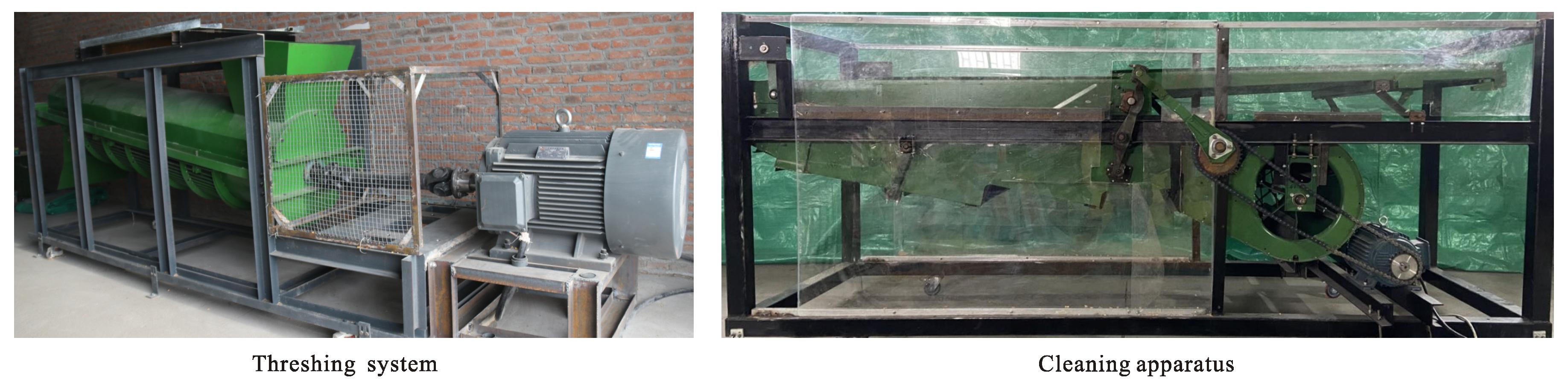
In this section, we first provide the materials utilized for the study. Then we describe the proposed method, including the algorithm of sieve dividing, the algorithm of blockage recognition. Finally, we introduce the metric to evaluate blocking level.

2.1. Material

The corns used for this study were harvested in Lishu city, China. The variety was Feitian 358 with 600 mm row spacing and 269 mm plant spacing, respectively. The used ears contain kernels with a moisture content of 27.3%.

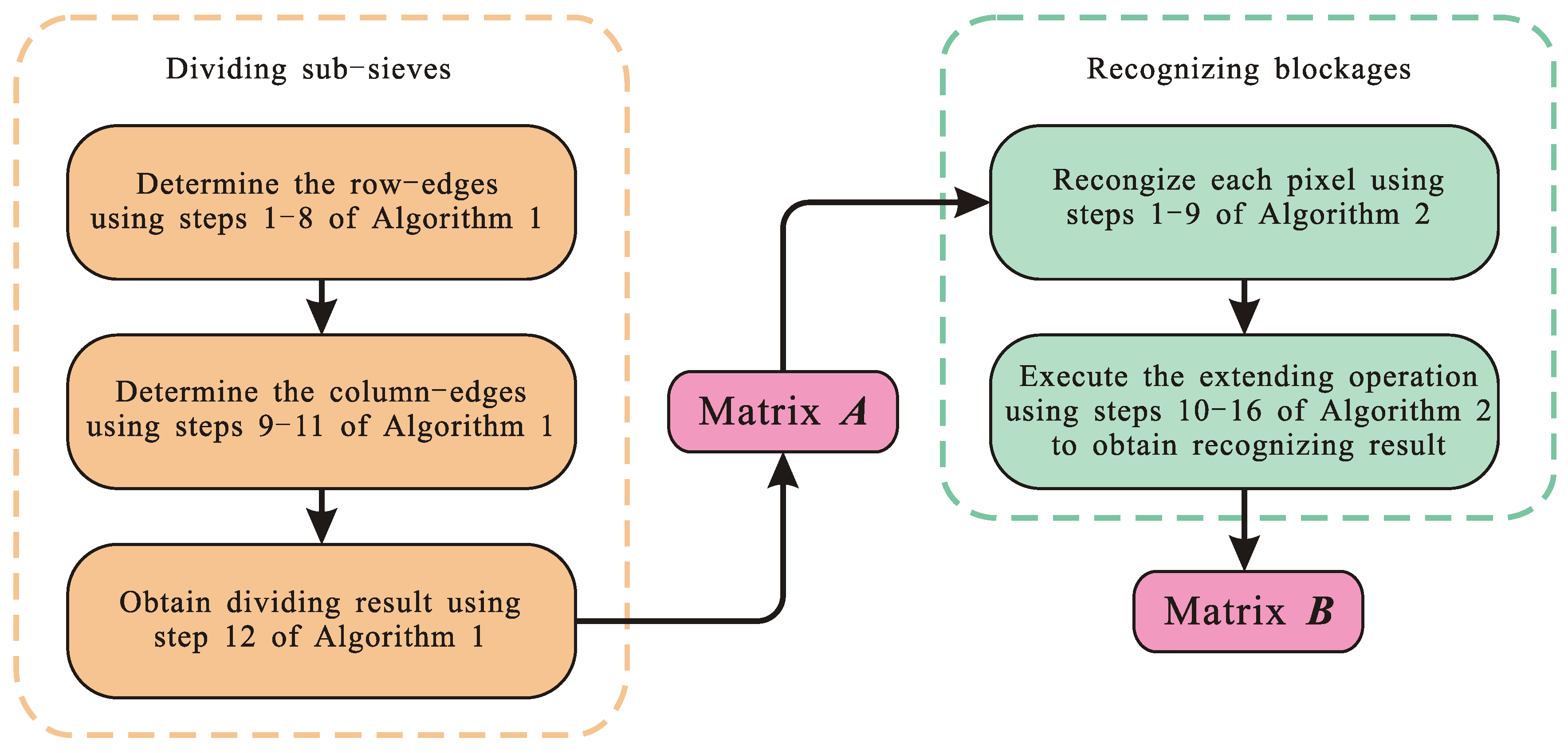
2.2. Algorithm of Sieve Dividing

As is shown in Figure 1a, the jittering sieve is composed of a set of tiered sub-sieves. In order to provide basis for automatic blockage cleaning, it is necessary to locate the blockages to the sub-sieves. Therefore, the first task of our study is to accurately divide the sieves. For this purpose, we develop a dividing algorithm that is summarized as Algorithm 1. The division of a sieve can be regarded as the problem to recognize the edges of each sub-sieve. For readable we provide an example while we introduce the algorithm. The original image with the spatial size of $600\times 500$ is presented in Figure 1a and it is denoted by $\underline{\mathit{X}}\in {\mathcal{R}}^{n_1\times n_2\times 3}$. Let its first order and second order represent the row and column, respectively. We first recognize the row edges. The strategy is based on the fact that the luminance of the pixels in row edges is obviously lower than that in other positions. In other word, if we denote ${\mathit{e}}_{row}\in {\mathcal{R}}^{n_1}$ and $\mathit{e}=\parallel \underline{\mathit{X}}{(i,:,:)\parallel }_F$, the indexes of minimums in ${\mathit{e}}_{row}$ should indicate the row edges, and these minimums show the approximate cyclicity as the widths of sub-sieves are close. To avoid the choice of minimums that do not indicate row edges, the cyclicity, $c_{row}$, should be determined. For this purpose we utilize the zero-centering operation to ${\mathit{e}}_{row}$ (step 6 of Algorithm 1), and then use the trigonometric function to fit it. This procedure is shown in Figure 1b. Next, we select the minimums of ${\mathit{e}}_{row}$ based on the constraint that two adjacent points are at least $0.85c_{row}$ apart, and the result is presented in Figure 1c, where the indexes of red points, written as ${\Gamma }_{row}$ indicate the positions of row edges.

Algorithm 1: Dividing jittering sieve into sub-sieves

Require: Original RGB image $\underline{\mathit{X}}\in {\mathcal{R}}^{n_1\times n_2\times 3}$, aspect ratio of sub-sieves $\mu$. 1: Initialize matrix $\mathit{A}=\mathit{0}\in {\mathcal{R}}^{n_1\times n_2}$; 2: Initialize vector ${\mathit{e}}_{row}\in {\mathcal{R}}^{n_1}$; 3: for each row $i\in \{1,2,\cdots ,n_1\}$ do 4:  Denote ${\mathit{X}}_i=\underline{\mathit{X}}(i,:,:)$ and compute ${\mathit{e}}_{row}\left(i\right)={\parallel {\mathit{X}}_i\parallel }_F$; 5: end for 6: ${\mathit{e}}_{row}\leftarrow {\mathit{e}}_{row}-\mathrm{mean}\left({\mathbf{e}}_{\mathrm{row}}\right)$; 7: Utilize trigonometric function to fit ${\mathit{e}}_{row}$, obtaining the cycle $c_{row}$, ${\alpha }_{row}=0.03c_{row}$; 8: Find the minimums of ${\mathit{e}}_{row}$, and two adjacent minimums are at least $0.85c_{row}$ apart. The indexes of these minimums are denoted as ${\Gamma }_{row}$; 9: Denote $\underline{\tilde{\mathit{X}}}=\underline{\mathit{X}}({\Gamma }_{row},:,:)$, $c_{col}=\mu c_{row}$, ${\alpha }_{col}=0.03c_{col}$; 10: Repeat the strategy given in steps 2–5 to obtain the F-norms each column of $\underline{\tilde{\mathit{X}}}$, denoted as ${\mathit{e}}_{col}\in {\mathbb{R}}^{n_2}$; 11: Find the maximums of ${\mathit{e}}_{col}$, and two adjacent maximums are at least $0.85c_{col}$ apart. The indexes of these maximums are denoted as ${\Gamma }_{col}$; 12: For each element of ${\Gamma }_{row}$, denoted as ${\gamma }_{row}$, set the entries of the ${({\gamma }_{row}-{\alpha }_{row})}^{th}$ row to the ${({\gamma }_{row}+{\alpha }_{row})}^{th}$ row of $\mathit{A}$ to be 1; for each element of ${\Gamma }_{col}$, denoted as ${\gamma }_{col}$, set the entries of the ${({\gamma }_{col}-{\alpha }_{col})}^{th}$ column to the ${({\gamma }_{col}+{\alpha }_{col})}^{th}$ column of $\mathit{A}$ to be 1. Ensure: Dividing result $\mathit{A}$.

Next, our task is to determine column edges. The strategy is also based on the luminance difference between the column edges and other positions. The difference exhibits an enhancement in the row edges. Specifically, in the sub-tensor $\underline{\mathit{X}}({\Gamma }_{row},:,:)$, the luminance of the pixels in column edges, indicated by $\underline{\mathit{X}}({\Gamma }_{row},{\Gamma }_{col},:)$, is obvious higher than that in other positions. Hence, it is feasible to determine the position of column edges by searching for the column bands that own higher Frobenius-norms (F-norms), and the F-norms of each column band is computed by ${\mathit{e}}_{col}\left(j\right)={\parallel {\tilde{\mathit{X}}}_j\parallel }_F$, where ${\tilde{\mathit{X}}}_j=\underline{\mathit{X}}(:,j,:)$, ${\mathit{e}}_{col}\in {\mathbb{R}}^{n_2}$. Similarly to the selection of row edges, the approximate cycle of column edges is required to know. For this purpose, a widespread property can be employed, that is, the aspect ratio of all sub-sieves are approximately same for a jittering sieve. Assuming that the aspect ratio is approximate $\mu$, the cycle of column edges can be computed by $c_{col}=\mu c_{row}$. In practical, the spaces between adjacent column edges are not completely same. Therefore, we empirically suggest using $0.85c_{col}$ as the minimum interval for searching the maximums of ${\mathit{e}}_{col}$ to avoid missing of maximums. The parameter $\mu$ depends on the used jittering sieve, and it should be obtained as the prior information by measuring the approximate aspect ratio of sub-sieves. In this study $\mu$ is set to 5. The above strategies are summarized as steps 10 and 11 in Algorithm 1. The graphical representation for determination of column edges is provided in Figure 2a,b. Finally, we obtain the final dividing result as a binary image, of which the edges with a specified width are set to 1 and other positions are set to 0. The widths of row edges and column edges, ${\alpha }_{row}$ and ${\alpha }_{col}$, are set to $0.03c_{row}$ and $0.03c_{col}$, respectively. The dividing result is shown in Figure 2c.

2.3. Algorithm of Blockage Recognition

This subsection introduces the proposed algorithm of blockage recognition that is summarized in Algorithm 2. The blockages caused by kernels show an obvious difference with sieves in terms of RGB data, that is, the respective components of red, green, and blue bands. This is the theoretical basis of the proposed algorithm, for which we set the upper thresholds and lower thresholds, for reflectance values the three bands, respectively. The thresholds are the basis to search for kernel blockages. Specifically, for an arbitrary pixel of an objective image, expressed as $\mathit{x}=[x_r,x_g,x_b]=\underline{\mathit{X}}(i,j,:)$, if all three reflectance values, $x_r,x_g,x_b$, are within the intervals between their upper thresholds and lower thresholds, that is, ${\theta }_r<x_r<{\vartheta }_r$ and ${\theta }_g<x_g<{\vartheta }_g$ and ${\theta }_b<x_b<{\vartheta }_b$, the pixel is assumed to own the similar spectral reflectance to the kernel, and it is regarded to belong to kernel blockage. For all areas of the objective image except for row edges and columns, each pixel is classified by using steps 2–9 to obtain a preliminary recognizing result. In general, not all pixels of a kernel could satisfy the threshold constraint of three bands. Only part of pixels are successfully recognized in the preliminary result. Hence, we develop an expanding operation to obtain the accurate areas of blockage which is provided in steps 10–16. The extending operation is an iterative process. For each iterative cycle, all pixels that own at least $\lambda$ neighboured pixels with the value of 2 are set to 2. Here, the value 2 indicates that the pixel belongs to the recognized blockage. The neighboured pixels of are defined as the left-upper, the upper, the right-upper, the left, the right, the left-lower, the lower, and the right-lower pixels. The number of neighboured pixels of a common pixel is 8. The numbers are 5 and 3 for the pixels in the border and corner, respectively. The termination condition to quit the iteration is the maximum number of iterative cycles is reached or the outputted results do not change any more. To clearly illustrate the proposed method, we present the flowchart in Figure 3 where the steps of two algorithms are summarized into five main processes. The matrix $\mathit{A}$ is the intermediate result, and the matrix $\mathit{B}$ is the final result. The example of blockage recognition that is followed by Figure 2 is presented in Figure 4 with $\lambda =4$.

Algorithm 2: Recognizing of blockages

Require: Original RGB image $\underline{\mathit{X}}\in {\mathcal{R}}^{n_1\times n_2\times 3}$, dividing result $\mathit{A}$, upper thresholds ${\vartheta }_r,{\vartheta }_g,{\vartheta }_b$, lower thresholds ${\theta }_r,{\theta }_g,{\theta }_b$, parameter $\lambda$. 1: Initialize vector $\mathit{B}=\mathit{A}$; 2: for every spatial point $(i,j)$ do 3:  if $\mathit{A}(i,j)=0$ then 4:   Denote $x_r=\underline{\mathit{X}}(i,j,1)$, $x_g=\underline{\mathit{X}}(i,j,2)$, $x_b=\underline{\mathit{X}}(i,j,3)$; 5:   if ${\theta }_r<x<{\vartheta }_r$ and ${\theta }_g<x<{\vartheta }_g$ and ${\theta }_b<x<{\vartheta }_b$ then 6:    ${\mathit{B}}_{i,j}=2$; 7:   end if 8:  end if 9: end for 10: while the termination condition is not reached do 11:  for each pixel of $\mathit{B}$, $\mathit{B}(i,j)$ do 12:   if more than $\lambda$ of its neighboured pixels equal to 2 then 13:    $\mathit{B}(i,j)\leftarrow 2$; 14:   end if 15:  end for 16: end while Ensure: Recognizing result $\mathit{B}$.

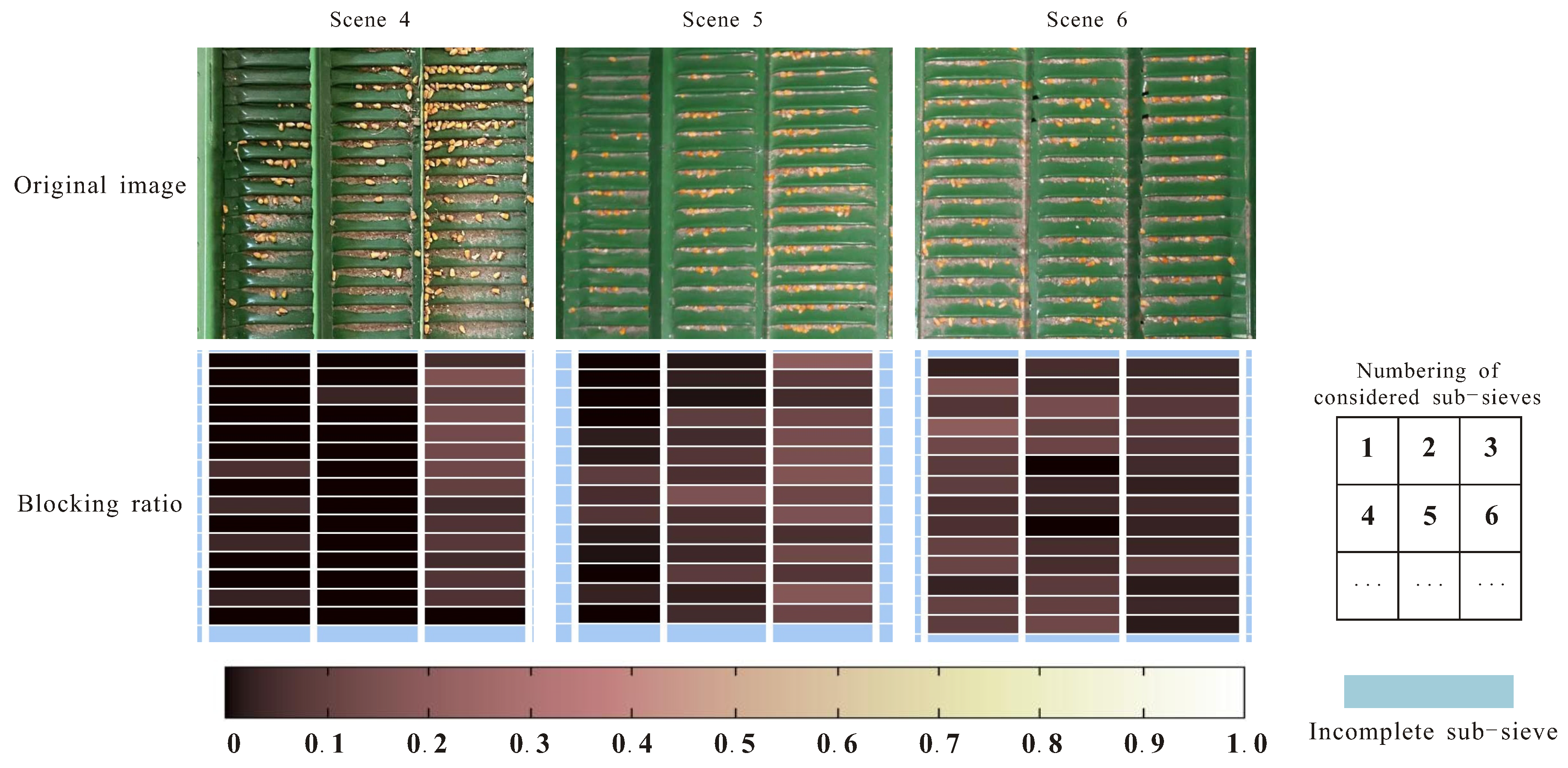
2.4. Evaluation of Blocking Level

This subsection introduces the metric for the evaluation of blocking level. The result combining sieve division and blockage recognition is shown as Figure 5b, where the recognized sieve edges and blockages are presented in white and blue, respectively. The metric, blocking ratio, denoted as $\gamma$, is proposed to evaluate the blocking level for each sub-sieve, and it is defined as the area proportion of blockage in a sub-sieve. The measurement of $\gamma$ is realized by calculating the number of pixels of recognized blockages and that of the corresponding sub-sieve. The result to compute the blocking ratio for each sub-sieve shown in Figure 5b is presented in Figure 5c, where the blocking levels are indicated by different colors.

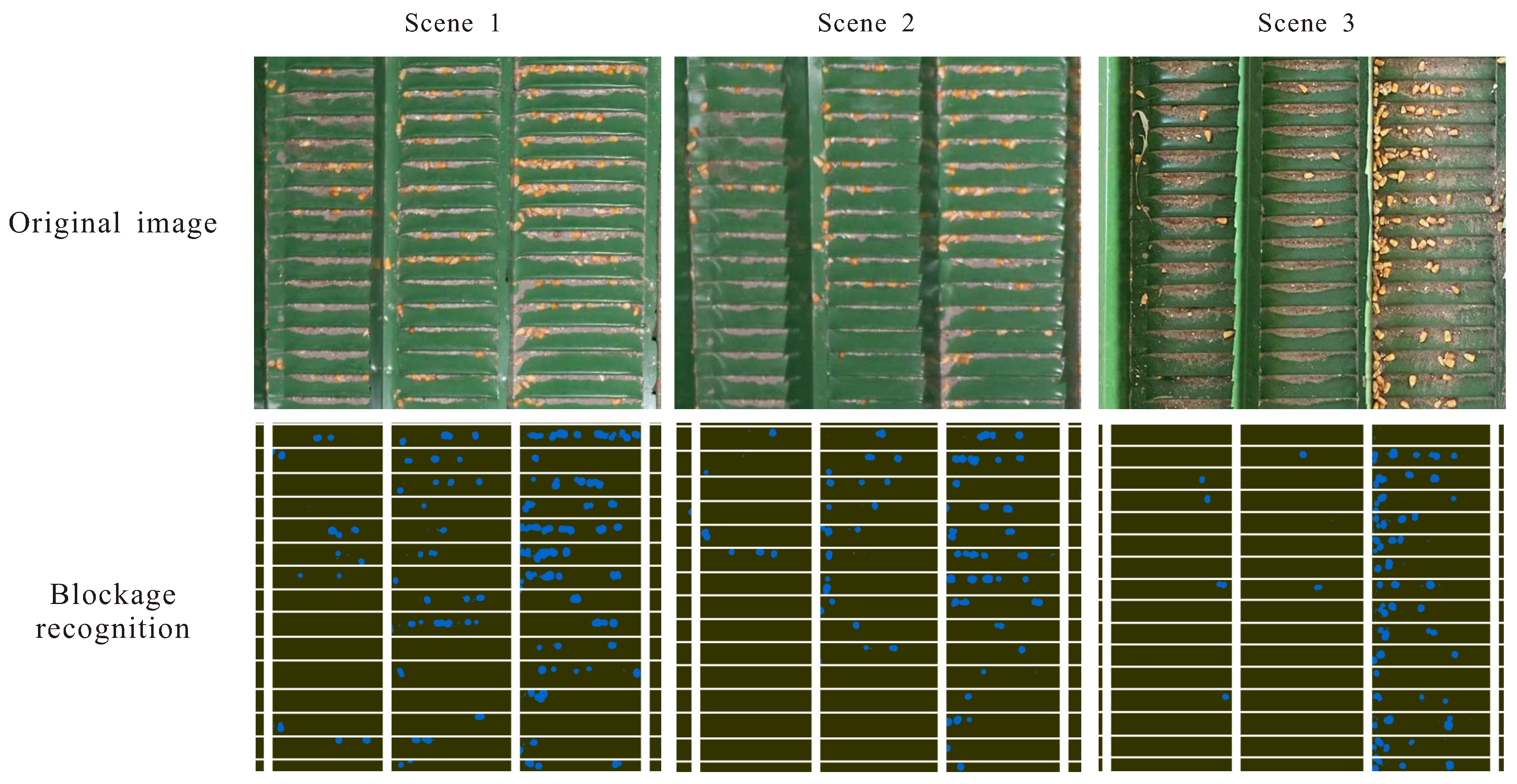
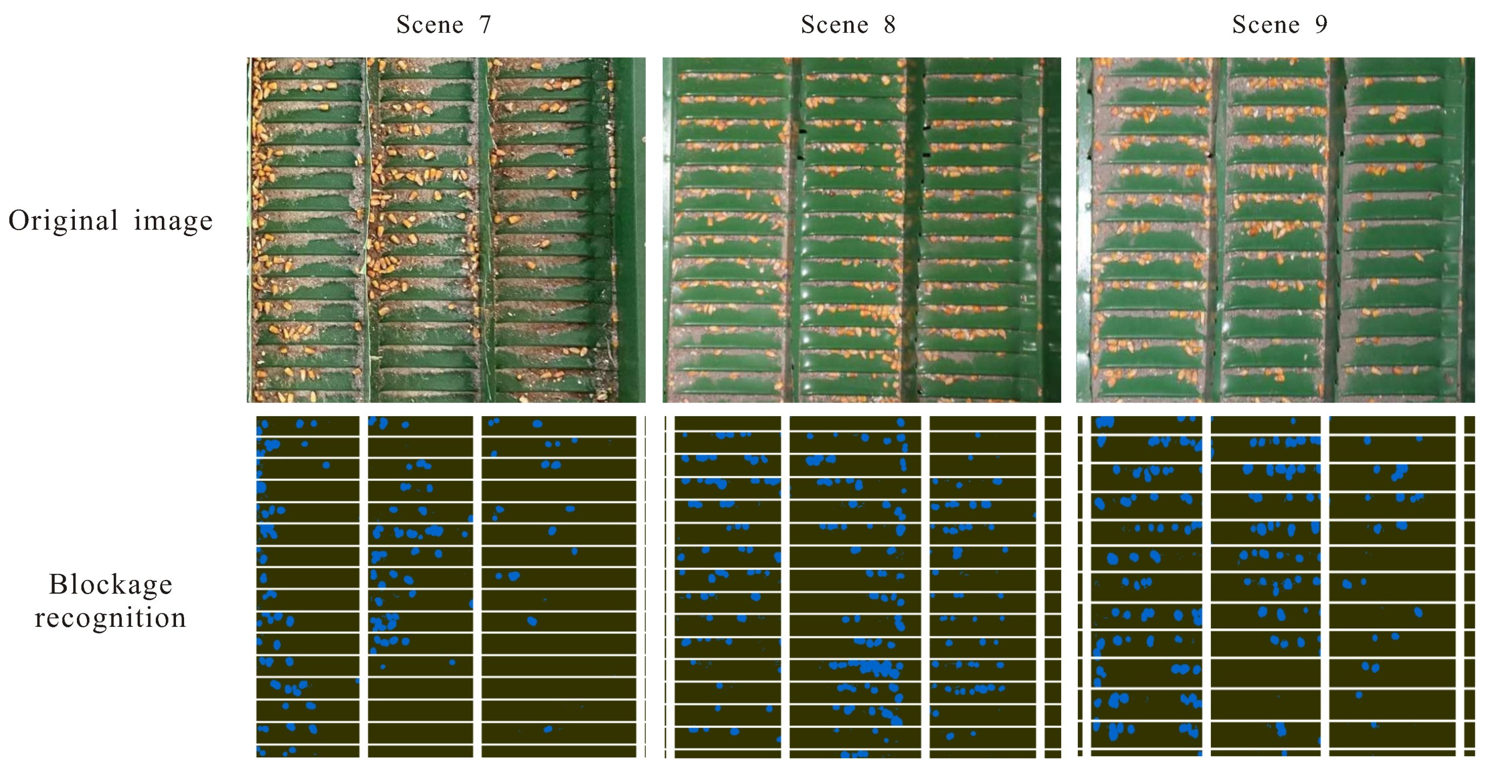
3. Experimental Results and Analysis

This section provides the experimental results and analysis. To start, we introduce the source of experimental scenes. Figure 6 shows the threshing system and the cleaning apparatus that were utilized in this study. The corn ears introduced in Section 2.1 were first put into threshing system to obtain the mixtures of kernels and impurities. Then pure kernels were separate from impurities through the cleaning apparatus. The cleaning apparatus is the original model of the John Deere 3316 harvester, such that it could simulate actual harvesting. We considered three rotational speeds of the threshing system, 400 rpm, 500 rpm, and 600 rpm, as they are the common rotational speeds in practical. For each rotational speed, we randomly selected the point-in-time to halt the cleaning process to acquire 3 test scenes. Thus, totally 9 scene were used for experiments. Scenes 1–3, 4–6 and 7–9 were acquired with the rotational speed of 400 rpm, 500 rpm, and 600 rpm, respectively. These scenes contained different parts of the jittering sieve of the cleaning apparatus with blockages. Higher rotational speed was set with higher feed quantity. The increase of feed quantity improved the kernel throughput on the jittering sieve per unit time, leading to the aggravation of kernel blocking. The images were processed by using the Matlab software platform on a personal computer.

For each scene, we first divided the sieve into sub-sieves by using Algorithm 1. The aspect ratio $\mu$ was set to 5 due to the size of jittering sieve. Then, we recognized blockages by using Algorithm 2. The parameter $\lambda$ was set to 4. The maximum number of iterative cycles of expanding operation was set to 3. The lower thresholds ${\theta }_r,{\theta }_g,{\theta }_b$ were set to 230, 160, and 0, respectively (the data were 8-bit). The upper thresholds ${\vartheta }_r,{\vartheta }_g,{\vartheta }_b$ were set to 255, 255 and 140, respectively. Finally, we computed the blocking ratios for each sub-sieve of each scene, and compared the results to the actual blocking levels.

The original objective images of test scenes and their dividing results are shown in Figure 7, Figure 8 and Figure 9. To verify the performance of division, we compare the numbers of recognized row edges and column edges to the real ones, which are summarized in

Table 2. Summary on recognized row edges and column edges.

	Number of Row Edges	Number of Recognized Row Edges	Success Rate (%)	Number of Column Edges	Number of Recognized Column Edges	Success Rate (%)
Scene 1	15	15	100.00	4	4	100
Scene 2	15	15	100.00	4	4	100
Scene 3	16	16	100.00	4	4	100
Scene 4	16	16	100.00	4	4	100
Scene 5	15	15	100.00	4	4	100
Scene 6	15	15	100.00	4	4	100
Scene 7	15	15	100.00	4	4	100
Scene 8	15	15	100.00	4	4	100
Scene 9	12	12	100.00	4	4	100
Total	134	134	100.00	36	36	100.00

. It can be noted that for all scenes, all row edges and column edges were successfully recognized, such that all sub-sieves were accurately divided. The recognition of blockages is presented in Figure 10, Figure 11 and Figure 12 where the blue regions and white regions denote the recognized blockages and the sieve edges, respectively.

Next, we conducted the experiments on blocking level evaluation. Based on the sieve dividing results and the blockage recognizing results, we computed the blocking ratios of each sub-sieve by using the strategy given in Section 2.4. For readable, we presented the blocking ratio in different colors in Figure 13, Figure 14 and Figure 15. It could be noted the blocking ratios are obvious higher at the sub-sieves that contains more kernels. For better illustration of this issue, we then summarized the actual numbers of blocking kernels in each sub-sieve, aiming to verify the correlation between the actual blocking level and the proposed metric.

Only the completely presented sub-sieves are considered. As shown in Figure 13, Figure 14 and Figure 15, they were numbering from left to right, and then from top to bottom. The incomplete sub-sieves were not considered in this part of experiments. The results are presented in Figure 16. The actual numbers of blockages of each sub-sieve are plotted in blue, and the blocking ratios of each sub-sieve are plotted in yellow. It can be noted that, for each scene the two curves are obvious consistent. We also employ the cross-correlation coefficient of the two variables [23], which is defined as

$$\begin{array}{c}\hfill \rho ({\mathit{y}}_1,{\mathit{y}}_2)=\frac{Cov({\mathit{y}}_1,{\mathit{y}}_2)}{\sqrt{Var\left({\mathit{y}}_1\right)Var\left({\mathit{y}}_2\right)}},\end{array}$$

(1)

where ${\mathit{y}}_1$ and ${\mathit{y}}_2$ denotes the vectors that contains the value of blocking ratio and the actual number of blocking kernels, respectively. The notations, $Cov(·)$ and $Var(·)$ represent the covariance and the variance, respectively. The value of $\rho$ will be 1 when ${\mathit{y}}_1$ and ${\mathit{y}}_2$ are completely relative. Among all 9 test scenes, the maximum value and the minimum value of $\rho$ are 0.961 (scene 3) and 0.882 (scene 6), respectively. For 8 of 9 scenes, the values of $\rho$ exceed 0.9. The mean value of $\rho$ for all test scenes is 0.932. Obviously, the blocking ratio has a high linear correlation to the actual number of blocking kernels. The results demonstrate the blockages of each sub-sieve proposed algorithms can be accurately recognized by using the proposed algorithms, and the proposed metric is appropriate to evaluate the blocking level.

4. Discussions

In this section, we first discuss the limitation of this study. Next, we provide the prospect for future work to address existing limitations.

4.1. Limitations

In this study, we implemented the proposed method by using the hardware of John Deere test rig and the Matlab-based software on personal computer. The experiments verified the performance of the proposed algorithms and the metric. However, there are still some limitations of this study. First, the features of test scenes were similar. The variety of test scenes were limited as they were all derived from our cleaning apparatus. To further test the performance of the proposed method, more experiments should be conducted by using the developed hardware for actual harvesters with cleaning apparatus that contains different features from the used one in this study. The features such as paint color, sub-sieve size, and lights require more consideration. Second, in this study the sieves in the test scenes are orthogonal to the coordinates such that directly using Algorithm 1 is able to accurately find sub-sieves in a jittering sieve. However, the acquired images may not be completely orthogonal to coordinates if the camera or jittering sieve is shaken while harvesting. In such case, the rotating operation should be executed before sieve division.

4.2. Future Work

For the purpose of portable application and online monitoring, the embedded-system-based hardware and software should be developed in the future. As presented in Figure 17. The implementation is composed of four parts, the RGB camera, the light source, the embedded system, and the host computer. The natural light source is suggested. It is because the proposed blockage recognition algorithm requires the thresholds of three bands to judge whether a pixel belongs to kernel blockage, and the natural light source could provide a standard light environment for the judgment. As indicated by step 5 of Algorithm 2, the judgment based on the thresholds may be influenced if the light is too weak or too strong. To address issue, the following improvements can be considered.

• Use the adjustable light source such that the thresholds can be tested and adjusted in advance.
• Normalize the RGB data of each pixel, that is, $\underline{\mathit{X}}(i,j,:)$, and then compute the correlation between the normalized data and the dictionary to judge whether the pixel belongs to kernel blockage. The dictionary is trained by using training samples, and various of dictionary learning methods can be employed for this purpose [24].

Besides a light environment, the paint color is another factor that may influence blockage recognition. Therefore, for better performance of recognition, painting jittering sieves a color that is obviously different from kernels is suggested.

The image processing system is composed of lower computer and upper computer, and they communicate wirelessly. The lower computer is realized by an embedded system with an RGB camera. The embedded computer module, Jetson TX2, is selected as the hardware of the lower computer. This module contains the graphics processing unit with 256 Nvidia cube cores, the Denver dual-core central processing unit, and the advanced reduced instruction set computer machine of A57 complex. For the purpose of portability, a storage battery is utilized to provide power for the motherboard. The software of lower computer is developed based on the Python programming language. Based on the software, the camera is controlled to acquire the image of the objection. The data of image is transferred to upper computer by using the Socket library.

The hardware of an upper computer can be realized by the normal personal computer. Therefore, the main development task of upper computer is the software that can be developed by the Python. The interactive interface contains the functions of start-stop, online monitoring, parameter input, and so forth. The data are transformed into images by using the V4L2 library, which is the genetic kernel driver for video devices of the Linux.

5. Conclusions

We have proposed a sieve dividing algorithm and a blockage recognition algorithm. The dividing algorithm, that is, Algorithm 1, is used to recognize sub-sieves and their edges from a jittering sieve. Algorithm 2 is used to recognize kernel blockages based on the dividing results obtained from Algorithm 1. For recognition, each pixel of the sub-sieves is first judged through the thresholding strategy, and then the extending operation is executed to determine the blocking area. We have also proposed the metric, the blocking ratio, to evaluate the blocking level by computing the area proportion of a blockage in a sub-sieve.

The performance of proposed algorithms and the metric have been verified based on the cleaning apparatus of the John Deere 3316 harvester with the jittering sieve in green. For the proposed sieve dividing algorithm, the determination of row edges and column edges is based on the luminance that is reflected by the F-norm of the corresponding matrix (see Step 4 of Algorithm 1). For the accuracy of blockage recognition, it is suggested to distinguish the sieve color from the kernel color.

The experimental results demonstrate all sub-sieves, as well as their row edges and column edges, can be correctly determined by using Algorithm 1. For all test scenes, the success ratio of edge determination reaches 100%. The results have also indicated the high correlation between the actual and recognized blocking areas. The mean cross-correlation coefficient of the blockage levels and the actual numbers of blocked kernels is 0.932. Indicated by the results, there is no obvious influence of the rotational ratio on recognizing accuracy. Overall, the proposed method has the potential to achieve automatic blockage detection for corn harvesters at work. We believe this study could also provide the basis for intelligent blockage clearing.

References

1. Esteves, C.A.C.; Colemanb, W.; Dubec, M.; Rodriguesa, A.E.; Pinto, P.C.R. Assessment of key features of lignin from lignocellulosic crops: Stalks and roots of corn, cotton, sugarcane, and tobacco. Ind. Crops Prod. 2016, 92, 136–148. [Google Scholar] [CrossRef]
2. Chen, S.; Chen, X.; Xu, J. Impacts of climate change on agriculture: Evidence from China. Ind. Crops Prod. 2016, 76, 105–124. [Google Scholar] [CrossRef]
3. Tabacco, E.; Ferrero, F.; Borreani, G. Feasibility of Utilizing Biodegradable Plastic Film to Cover Corn Silage under Farm Conditions. Appl. Sci. 2020, 10, 2803. [Google Scholar] [CrossRef]
4. Cheng, X.; Zhang, Q.; Yan, X.; Shi, C. Compressibility and equivalent bulk modulus of shelled corn. Biosyst. Eng. 2015, 140, 91–97. [Google Scholar] [CrossRef]
5. Isaak, M.; Yahya, A.; Razif, M.; Mat, N. Mechanization status based on machinery utilization and workers’ workload in sweet corn cultivation in Malaysia. Comput. Electron. Agric. 2020, 169, 105208. [Google Scholar] [CrossRef]
6. Mantovani, E.C.; de Oliveira, P.E.B.; de Queiroz, D.M.; Fernandes, A.L.T.; Cruvinel, P.E. Current Status and Future Prospect of the Agricultural Mechanization in Brazil. AMA-Agric. Mech. Asia Afr. Lat. Am. 2020, 50, 20–28. [Google Scholar]
7. Qian, F.; Yang, J.; Torres, D. Comparison of corn production costs in China, the US and Brazil and its implications. Agric. Sci. Technol. 2016, 17, 731–736. [Google Scholar]
8. Puzauskas, E.; Steponavicius, D.; Jotautiene, E.; Petkevicius, S.; Kemzuraite, A. Substantiation of concave crossbars shape for corn ears threshing. Mechanika 2016, 22, 553–561. [Google Scholar] [CrossRef]
9. Qu, Z.; Zhang, T.; Li, K.; Yang, L.; Cui, T.; Zhang, D. The design and experiment of longitudinal axial flow maize threshing and separating device. In Proceedings of the 2017 ASABE Annual International Meeting, Spokane, WA, USA, 16–19 July 2017. [Google Scholar]
10. Qu, Z.; Zhang, T.; Li, K.; Yang, L.; Cui, T.; Zhang, D. Experiment on distribution of mixture in longitudinal axial flow threshing separation device for maize. In Proceedings of the 2019 ASABE Annual International Meeting, Boston, MA, USA, 7–10 July 2019. [Google Scholar]
11. Chen, Y.; Chao, K.; Kim, M.S. Machine vision technology for agricultural applications. Comput. Electron. Agric. 2002, 26, 173–191. [Google Scholar] [CrossRef] [Green Version]
12. El-Mesery, H.S.; Mao, H.; Abomohra, A.E.F. Applications of non-destructive technologies for agricultural and food products quality inspection. Sensors 2019, 19, 846. [Google Scholar] [CrossRef] [Green Version]
13. Brosnan, T.; Sun, D. Inspection and grading of agricultural and food products by computer vision systems—A review. Comput. Electron. Agric. 2002, 36, 193–213. [Google Scholar] [CrossRef]
14. Zhang, L.; Geer, T.; Sun, X.; Shou, C.; Du, H. Application of hyperspectral imaging technique in agricultural remote sensing. Bangladesh J. Bot. 2019, 48, 907–912. [Google Scholar]
15. Eyarkai, V.N.; Thangave, K.; Shahir, S.; Thirupathi, V. Comparison of various RGB image features for nondestructive prediction of ripening quality of “alphonso” mangoes for easy adoptability in machine vision applications: A multivariate approach. J. Food Qual. 2016, 39, 816–825. [Google Scholar] [CrossRef]
16. Taghizadeh, M.; Gowen, A.A.; O’Donnell, C.P. Comparison of hyperspectral imaging with conventional RGB imaging for quality evaluation of Agaricus bisporus mushrooms. Biosyst. Eng. 2011, 108, 191–194. [Google Scholar] [CrossRef]
17. Karayel, D.; Wiesehoff, M.; Özmerzi, A.; Müller, J. Laboratory measurement of seed drill seed spacing and velocity of fall of seeds using high-speed camera system. Comput. Electron. Agric. 2006, 50, 89–96. [Google Scholar] [CrossRef]
18. Leemans, V.; Destain, M.F. A computer-vision based precision seed drill guidance assistance. Comput. Electron. Agric. 2007, 59, 1–12. [Google Scholar] [CrossRef] [Green Version]
19. Liu, C.; Chen, B.; Song, J.; Zheng, Y.; Wang, J. Study on the image processing algorithm for detecting the seed-sowing performance. In Proceedings of the 2010 International Conference on Digital Manufacturing & Automation, Changsha, China, 18–20 December 2010; pp. 551–556. [Google Scholar]
20. Liu, Z.; Wang, S. Broken corn detection based on an adjusted YOLO with focal loss. IEEE Access 2019, 7, 68281–68289. [Google Scholar] [CrossRef]
21. Fu, J.; Yuan, H.; Zhao, R.; Chen, Z.; Ren, L. Peeling Damage Recognition Method for Corn Ear Harvest Using RGB Image. Appl. Sci. 2020, 10, 3371. [Google Scholar] [CrossRef]
22. Liao, K.; Paulsen, M.R.; Reid, J.F. Real-time detection of colour and surface defects of maize kernels using machine vision. J. Agric. Eng. Res. 1994, 59, 263–271. [Google Scholar] [CrossRef]
23. Zhao, X.; Shang, P.; Lin, A. Distribution of eigenvalues of detrended cross-correlation matrix. EPL 2014, 107, 40008. [Google Scholar] [CrossRef]
24. Tosic, I.; Frossard, P. Dictionary Learning. IEEE Signal Process. Mag. 2011, 28, 27–38. [Google Scholar] [CrossRef]
Figure 1. Recognition of row edges. (a) Original image. (b) Trigonometric fitting result. (c) Selected minimums.
Applsci 10 06319 g001
Figure 2. Process of recognizing column edges and the final dividing result. (a) Presentation of X ˜ ̲ . (b) Selected maximums of e c o l . (c) Final dividing result.
Applsci 10 06319 g002
Figure 3. Flowchart of the proposed algorithm.
Applsci 10 06319 g003
Figure 4. Preliminary recognizing result and expanding result of test example. (a) Original image. (b) Preliminary recognizing result. (c) Final dividing result.
Applsci 10 06319 g004
Figure 5. Evaluation of blocking level. (a) Original image. (b) Sieve division and blockage recognition. (c) Blocking ratio of each sub-sieve.
Applsci 10 06319 g005
Figure 6. Used threshing system and cleaning apparatus.
Applsci 10 06319 g006
Figure 7. Dividing results of scenes with rotational speed of 400 rpm.
Applsci 10 06319 g007
Figure 8. Dividing results of scenes with rotational speed of 500 rpm.
Applsci 10 06319 g008
Figure 9. Dividing results of scenes with rotational speed of 600 rpm.
Applsci 10 06319 g009
Figure 10. Recognition results of scenes with rotational speed of 400 rpm.
Applsci 10 06319 g010
Figure 11. Recognition results of scenes with rotational speed of 500 rpm.
Applsci 10 06319 g011
Figure 12. Recognition results of scenes with rotational speed of 600 rpm.
Applsci 10 06319 g012
Figure 13. Blocking level evaluating results of scenes with rotational speed of 400 rpm.
Applsci 10 06319 g013
Figure 14. Blocking level evaluating results of scenes with rotational speed of 500 rpm.
Applsci 10 06319 g014
Figure 15. Blocking level evaluating results of scenes with rotational speed of 600 rpm.
Applsci 10 06319 g015
Figure 16. Blocking ratio versus number of blocking kernels. (a) Scene 1. (b) Scene 2. (c) Scene 3. (d) Scene 4. (e) Scene 5. (f) Scene 6. (g) Scene 7. (h) Scene 8. (i) Scene 9.
Applsci 10 06319 g016
Figure 17. Outline of hardware implementation.
Applsci 10 06319 g017