Abstract
The research domain of device-free localization (DFL) is centered on the study of localization techniques which do not require targets to wear any kind of device. Passive radio mapping or passive fingerprinting is an example of a training-based DFL technique which uses the impact of a human target on radio frequency (RF) communication between stationary nodes to perform localization. We describe a set of experiments performed in a 42 m empty office environment in which we installed a RF network with nodes communicating on the 433 MHz and 868 MHz bands. We attempted to locate a single stationary human target based solely on signal strength measurements and did so for six different participants using two different fingerprinting methods. One method was based on Euclidean distance minimization while the other made use of a naive Bayesian classifier. We investigated the impact of frequency band, number of nodes and target body type on localization accuracy. Results indicated that a root mean square error of 48 cm could be obtained with only four nodes, provided that the data from both frequency bands was combined. Additionally, we investigated the potential of these fingerprinting approaches to distinguish between targets based on body type and perform a rudimentary form of passive identification. Accuracy rates for identification could vary significantly depending on target location, with results ranging from 0.07 to 0.75 in the exact same environment. However, the experiment participant with the lowest height and weight could be distinguished from the other participants in over 90% of cases.
1. Introduction
The term "device-free localization" (DFL) refers to the use of technologies which enable the automatic localization of human and/or nonhuman targets, without requiring the targets to carry a device or tag. While there is a wide variety of localization approaches which fall under the umbrella of DFL, ranging from differential air pressure-based techniques [1] to techniques which make use of floor vibrations [2], the term is often used in the context of Radio Frequency (RF)-based DFL. In this approach, the impact of the physical presence of targets on RF-waves within an environment is used to infer location-related information about them.
The research domain of device-free localization was formally defined for the first time in 2007 by Youssef et al. [3]. They considered DFL to consist of primarily three aspects: detection, tracking and identification. Detection refers to determining whether there are any entities present causing changes in the environment and if so, how many entities there are. Tracking refers to estimating the actual locations of these entities and the manner in which these evolve over time. Finally, identification refers to determining identity-related information regarding these entities. The term "identity" in this context is loosely defined and can refer to both physical characteristics (e.g., size, mass or main material) or to an actual human identity. This aspect in particular was considered to be exceptionally difficult and was referred to as "the identification problem".
In the years since the aforementioned seminal study was published, significant advances have been made within this field of research. Many different techniques have been developed which focus on one or more of the three main aspects [4]. While initial approaches tended to solely make use of the impact of targets on the Received Signal Strength (RSS) of RF signals, an increasing number of studies is focused on other signal descriptors—most notably Channel State Information (CSI) [5]. CSI provides both amplitude and phase information for each subcarrier in RF communication which makes use of Orthogonal Frequency Division Multiplexing (OFDM). Its increasing use within DFL is primarily fueled by the increasing ease with which one can obtain this data from commercially available Wi-Fi equipment [6]. In recent years, CSI-based approaches have even led to the creation of identification systems which can differentiate between individuals based on the manner in which their unique gait leads to different measurement patterns [7,8,9]. It should be noted, however, that this assumes the availability of the necessary bandwidth for these signals. This is not feasible for every application and/or environment and purely RSS-based DFL systems are still an active topic of research [10,11].
One popular approach which was already used by Youssef et al. [3] to illustrate the feasibility of DFL as a concept, is called passive radio mapping or passive fingerprinting. The basic concept of this method is similar to its active fingerprinting counterpart. A training-based radio map (or fingerprint database) is constructed which links possible target locations to corresponding sets of measurements. When the system is online, live measurements are compared to the fingerprint database and the closest matches are then assumed to be indicative of locations which are near the true target location. For the active approach, measurements based on RF links between a device attached to the target and stationary nodes installed within the environment are used. In contrast, passive fingerprinting makes use of the RF-communication between the stationary nodes, which is impacted differently based on the target location(s). Existing research shows that RSS-based passive fingerprinting systems can accurately locate human targets in large and complex environments with a surprisingly small number of stationary nodes. In 2012, Seifeldin and Youssef created the Nuzzer system [12] which was capable of locating a single human target with a median error of 1.82 m in an office building floor which had a total area of approximately 1500 m. Only three 802.11b access points and two consumer-grade laptops were used as stationary nodes, leading to a total of six one-way communication links. The fingerprint matching algorithm primarily consisted of a Naive Bayesian classifier which made use of the RSS-values reported by the network interface cards (NICs). Much more complex systems have been developed in the years since, such as SCPL (sequential counting, parallel localizing) [13] and ACE [14] which allowed for robust multitracking without requiring manually constructed fingerprints for each possible combination of target locations.
In [15], Mager et al. investigated the longevity of passive fingerprint databases in relation to changes within the environment. While they were not the first to investigate this aspect [16], their research showed the magnitude of this issue. Through the combination of a random forest classification algorithm with RSS measurements which were performed on multiple frequency channels within the 2.4 GHz band, they managed to mitigate this problem. In [17], Lei et al. improved upon this research by improving the channel selection algorithm and using a logistic regression classifier instead of random forests.
Despite these advances, there are still many unanswered questions within this field of research. The previously mentioned requirement to regularly update the fingerprint database when the presence and/or location of static objects changes still remains a major disadvantage of passive fingerprinting techniques. Additionally, there have only been very limited investigations into the potential impact the body type of the human target can have on the localization accuracy.
In this paper, we describe the passive fingerprinting experiments we performed in a 42 m environment which contained fifteen 433 MHz and 868 MHz nodes and analyze the results. We defined fifteen locations within this environment and had multiple participants of differing height and weight stand at each of these locations while RSS-measurements were performed. Two sets of measurements were performed. In the first set, the measurement duration for one individual standing at a specific location lasted for thirty seconds. During this period, the person was instructed to move in a stationary manner. Each measurement for the second set lasted for only ten seconds and the person was instructed to stand still alongside a single orientation. The first set was used to create a fingerprint database and the second was used for evaluation.
In our analyses of the resulting data, we investigated the following research questions:
- What impact does the number of nodes have on the localization accuracy? Based on existing literature, we expect the maximum number of nodes in our experiment (15) to be far beyond what is required to be sufficiently accurate.
- Are there any benefits to the use of sub-GHz frequencies? While 2.4 GHz is very common within DFL in general, sub-GHz frequencies have been successfully used within the field of passive fingerprinting. Is it useful to combine multiple frequencies in a single system?
- What is the impact of the body type of a human individual who is present in the environment on the localization accuracy? What if the individual whose presence was used to construct the fingerprint database differs significantly from the human present in the environment while the system is active?
- How feasible is it to differentiate between multiple individuals with different body types based on the impact on RSS measurements between the stationary nodes? Can a rudimentary form of identification be implemented?
In regards to this final research question, it is only in recent years that any progress has been made towards solving the identification problem within (noncamera based) DFL. As previously mentioned, the approach that is often used is based on the unique gait of the individuals between which one wants to differentiate. However, the use of only RSS does not suffice as a signal feature for these types of systems. Instead, they all require CSI measurements. The WiDisc system proposed by Scholz et al. [18] is one of the very few examples of an RSS-only identification system. The authors attempted to differentiate between a child, a woman and a tall man using four IEEE 802.15.4 transceivers communicating on the 2.4 GHz band in a 4.04 m by 5.33 m by 2.70 m lab environment. They used a deterministic passive fingerprinting method and managed to correctly estimate the presence of the child, woman and tall man respectively 43 %, 71 % and 86 % of the time. While these results indicated the feasibility of differentiating between these three size-based categories, it was quite clear that the system required further development and this was stated by the authors as well.
While the information provided by only using signal strengths is likely to be insufficient to match the capabilities of CSI-based systems, even a limited form of identification could still prove to be very beneficial and potentially enable interesting applications. An example would be a safety system which can detect the presence of children in industrial environments. Furthermore, the information provided by such a differentiation system would likely aid tracking approaches as well.
The remainder of this paper is structured as follows. In Section 2, we describe our experimental setup in detail and discuss our approach in analyzing the results, both in regards to localization and identification. In Section 3, we perform our localization for different combinations of frequency bands, number of nodes, classification algorithms and individuals used in the construction of the fingerprint database. Section 4 details our identification approach. Finally, in Section 5 a conclusion is presented in addition to an overview of our plans regarding future research.
2. Experimental Setup and Methodology
In this section we discuss the RF sensing network and the experimental environment in which it was installed. We describe the participants and the instructions they received over the course of the experiment. Finally, the classification approaches that were used for fingerprinting are detailed as well.
2.1. Construction of a Sub-GHz Passive RF Sensing Network
The RF sensing network we install consists of 15 regular nodes which are attached to tripods at a height of approximately 1.10 m. Each node consists of a plastic casing containing two battery-powered transceiver modules for respectively 433 MHz and 868 MHz. The transceivers for both frequency bands operate independently of each other and can therefore be considered to belong to two entirely separate networks which operate in an identical manner. Figure 1 shows a photograph of a node.
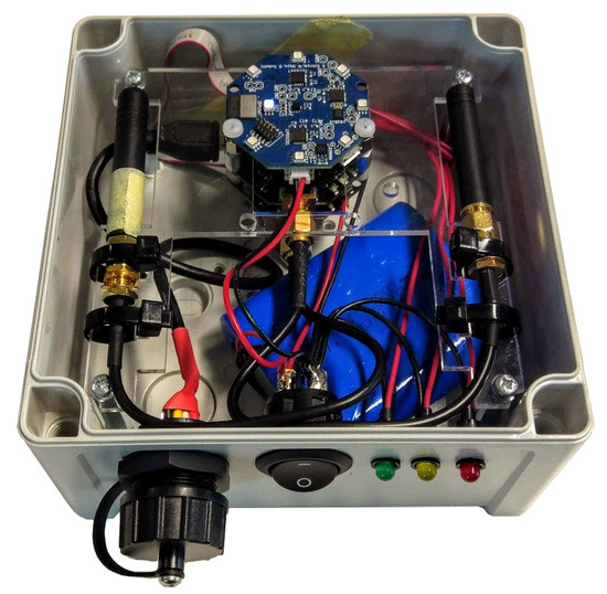
Figure 1.
A photograph showing the inside of a regular network node. It contains two OCTA-mini transceivers for respectively 433 MHz and 868 MHz communication attached to two antennas and a 6600 mAh battery.
Communication uses the DASH7 Alliance Protocol (D7A) [19] and is cycle-based. Each node is assigned a unique node id which determines the order in which they will broadcast a message to all other nodes. Upon receiving this message, a node will store the RSS with which it was received in an internal list at the index corresponding to the node id of the transmitting node. When a node’s turn to broadcast has arrived, the message it transmits will contain this list. A special type of node called the controller continuously listens to all communication within the network and passes on all of the RSS data to a laptop to which it is connected. Once all nodes have broadcasted, the cycle begins anew.
In addition to collecting and passing on the RSS measurements, the controller is also responsible for the timing of the communication described in the previous paragraph. At the beginning of each cycle, it will transmit a specialized start message and this will instruct each node that its moment to broadcast occurs at a specific time after receiving this message which is determined by the node id and the network parameter wtime. This parameter defines the period of time between transmissions of two subsequent nodes. In order to minimize the delay between an RSS measurement being performed and the data being passed on to the controller, it is important for wtime to be as small as possible. For the experiments described in this paper, wtime was equal to approximately 10 ms. The controller can also be instructed via the laptop to stop (or resume) periodically transmitting start messages and therefore halt (or resume) all network communication. Additionally, it can also instruct all network nodes to reset themselves and/or request new configuration parameters from the configurator. The configurator is a final, third type of node which contains all necessary parameters related to network communication (e.g., wtime, frequency channel, network size and node ids for every node). This node consistently listens for configuration requests from regular nodes and responds with the required information. A regular node will send these requests shortly after boot—only after it has received the necessary parameters can it participate in regular communication cycles. All communication related to configuration occurs on a separate frequency channel so that it will not interfere with regular operation.
The main advantage of this system architecture is the flexibility it provides. One only needs to change the relevant parameters in the configurator to add/remove nodes, increase/decrease the wtime parameter or change the frequency channel on which the cycle communication occurs. For our future development of the system, we are planning on incorporating the functionality of the configurator into the controller node.
2.2. Passive Fingerprinting Techniques
The RF sensing network described in the previous subsection consists of a maximum of 15 nodes, which leads to a total of 210 RSS values that are communicated to the controller during each cycle. Each communication link formed between two nodes is associated with two of these values; one for each direction in which communication can occur. We average these two values for each link and create a measurement vector with a length of 105 elements. This measurement vector forms the core aspect of our fingerprinting approaches.
As is the case for all fingerprinting techniques, the first step consists of a training phase in which a fingerprint database is created. These contain entries for each possible state (locations in Section 3 and identities in Section 4) and during the next step the goal is to try to match measurement vectors to the correct entry. We attempt to do so through two different methods outlined in the next paragraphs.
Our first approach makes use of the minimization of the Euclidean distance between the measurement vector and fingerprint database vectors associated with all possible states. Each fingerprint database vector is created by taking the average of the measurement vectors collected during the training phase when a target was present in the corresponding state. This is a classic fingerprinting technique—both for active and passive cases—whose results are often used as a baseline [12,16].
The distance between measurement vector whose data was collected when a single target was present in an unknown state s and the fingerprint database entry which corresponds to a certain state x can be described mathematically as
with m equal to the length of the measurement vector. It should be noted that all RSS values within our measurement vectors are in dBm.
The goal of this approach is to find the database entry state x which satisfies the following condition and is therefore assumed to correspond to the actual state s:
In our second approach, we make use of a naive Bayesian classifier for which we consider all elements of the measurement vector to be independent features. The goal of this approach is to maximize the probability for which an active measurement vector corresponds to a fingerprint database defined state x. Using Bayes’ theorem, this can be described as
We assume each state x to be equally probable, so therefore this equation can be rewritten as
Finally, due to the fact that we consider all features to be independent, can be calculated by the following formula:
with m equal to the length of the measurement vector.
In the fingerprint database, each state is represented by a number of Gaussians equal to the length of the measurement vectors. These functions show the distribution of RSS values for each link given that a target is present in a certain state and are created during the training phase by fitting the collections of RSS values to Gaussian distributions. They can then be used to calculate for each possible database defined state x, after which the highest probability is assumed to correspond to the actual state.
Both the minimization of Euclidean distance and the naive Bayesian classifier approaches are quite standard within the domain of passive fingerprinting. Much more advanced techniques do exist and have been successfully implemented within the state of the art [15,17]. However, the focus of this paper is not on the implementation of an advanced fingerprinting algorithm and we consider this to be currently out-of-scope.
2.3. Experiment Environment and Description
We installed our RF sensor network and performed our experiments in a 42 m office environment. Tables and other furniture were present near the windows, but the vast majority of the environment was unobstructed. Fifteen small, colorful cones were placed inside the environment to indicate possible locations where targets could be present. A schematic overview of the node locations and potential target locations is shown in Figure 2. Figure 3 shows a photograph of the environment.
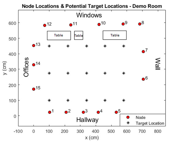
Figure 2.
A schematic overview of the experimental environment.
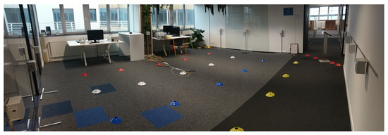
Figure 3.
A photograph of the office environment. It should be noted that both the nodes and cones had not yet been placed in their final locations as indicated by the schematic overview in Figure 2.
Each experimental measurement consisted of a human target being present at one of the fifteen locations indicated by the cones, while the RF sensor network collected RSS data. The duration of a measurement depended on whether the data was to be used for training (fingerprint database creation) or for evaluation. Training measurements lasted for 30 s during which the participant was instructed to randomly rotate and move in place. Each evaluation measurement took only 10 s and the participants had to stand still while facing the offices shown in the photograph in Figure 3. In practice, this led to approximately 50 measurement vectors for each evaluation measurement and 150 measurement vectors for each training measurement.
Figure 4 uses data from the 868 MHz 30-second training measurements to illustrate the impact the presence of a target can have on the signal strengths of the communication links, which is the crux of the entire passive fingerprinting technique. This figure shows the average RSS values with which communication between node 1 and every other node occurs, for four different locations at which a target could be present. The impact of target presence in the direct line-of-sight of a link tends to be rather intuitive. For example, when a target is present in the upper or lower left corner of the environment, the link formed by nodes 1 and 12 is attenuated by 4 to 7 dB when compared to a target being present in the upper or lower right corner. Less intuitive differences which are likely the result of complex multipath effects exist as well, as illustrated by the link between nodes 1 and 4. When a target is present in the lower left corner, the link is attenuated by 3 to 4 dB when compared to all other scenarios, despite the target not being located in the direct line-of-sight. A major advantage of a fingerprinting approach lies in the fact that all of these aspects do not need to be explicitly modeled.
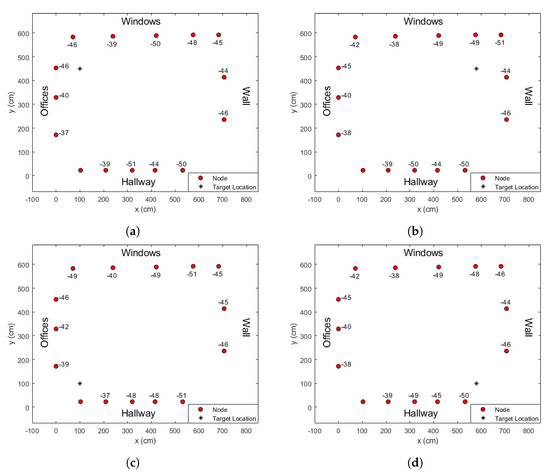
Figure 4.
Average Received Signal Strength (RSS) values with which communication between node 1 and every other node occurs, for four different locations at which a target could be present. The target is present near the upper left corner of the environment in (a), the upper right corner in (b), the lower left corner in (c) and the lower right corner in (d). All RSS values are in dBm.
For all of our experiments, we had the help of six volunteers who acted as human targets. Some of them differed significantly from each other in regards to body type. Table 1 shows the weight and height of each participant as measured at the time of the experiments. Training measurements were performed for four of the participants, while evaluation measurements were performed for all 6. The main reason for doing so was that we also wished to investigate the presence of targets for whom no training data existed.

Table 1.
Height and weight of the six volunteers who participated in our experiments.
All of the collected RSS data was stored in a database from which it could be retrieved for later analysis.
An overview of the most important experiment parameters can be found in Table 2. In the next section, we will describe the analyses we performed regarding target localization.
Table 2.
An overview of the most important experiment parameters. Transmission power refers to the output power as configured in the devices.
3. Sub-GHz Passive Localization
When analyzing the results, our initial focus lies with the most common use of passive fingerprinting approaches—target localization. First, we completely ignore the fact that the training measurements were performed for multiple targets and simply create a single fingerprinting database for which each location-based entry was created based on data from all six targets. Next, we investigate what happens when a fingerprint database is created based on data from only a single human individual and whether there are any decreases in accuracy when the body type of the training participant differs significantly from the evaluation participant.
Throughout this paper, we will focus on the accuracy rate as a key metric. It is defined as the ratio of the number of correct state estimations to the total number of state estimations. For localization results, we provide error distance metrics as well, although we consider them to be less important due to the fact that we assume discrete states (i.e., no target was ever present outside of the 15 predefined locations).
Additionally, we perform all of these analyses for multiple combinations of frequency bands, fingerprinting techniques and number of nodes. In regards to frequency bands, we determine separate accuracy rates using data from only the 433 MHz network, from only the 868 MHz network and from a combination of both. This combination occurs by simply appending the corresponding measurement vectors and fingerprint database entries from both networks to each other. We also determine separate accuracy rates for the two fingerprinting techniques discussed in Section 2.2—minimization of Euclidean distance and naive Bayesian classifier. Finally, because the number and exact positions of nodes can have a significant impact on localization accuracy within DFL in general [20,21,22], we wish to investigate this aspect as well. Given the impressive results which have been obtained in much larger environments with a very limited number of nodes within the state of the art, we strongly suspect 15 nodes to be far beyond what is required to allow for accurate localization. However, by virtually removing nodes through ignoring their RSS measurements and corresponding elements in the fingerprint database, we can obtain localization accuracies for the number of nodes varying from 2 to 15. Because each number of nodes has a large number of possible node combinations, we randomly select 100 combinations and calculate the localization accuracy for each of them. For this reason, we will primarily depict our localization results for each number of nodes as a boxplot created from the accuracy rates from these 100 selected node combinations. The only exceptions to this are 14- and 15-node scenarios, for which respectively only 15 and 1 possible combinations exist.
3.1. Constructing a Single Fingerprinting Database Based on All Training Data
As explained in the preceding paragraphs, we begin with the construction of a single localization fingerprint database based on the training measurements from all experiment participants. Next, we randomly select 25 measurement vectors from each evaluation measurement. Because we performed evaluation measurements at 15 locations with six different participants, this gives us a total of 25 × 6 × 15 = 2250 measurement vectors. We apply the previously discussed Euclidean and Bayesian fingerprinting techniques to this data for all possible combinations of frequency bands and number of nodes. The resulting accuracy rates and root mean square errors for 433 MHz, 868 MHz and a combination of both are respectively shown in Figure 5, Figure 6 and Figure 7.
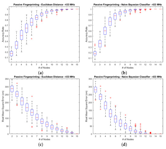
Figure 5.
Box plots of the accuracy rates and root mean square distance errors based on 433 MHz data. (a) and (b) show the accuracy rates for respectively the Euclidean distance-based and naive Bayesian classifier-based methods, while (c) and (d) show the root mean square distance errors for both approaches.
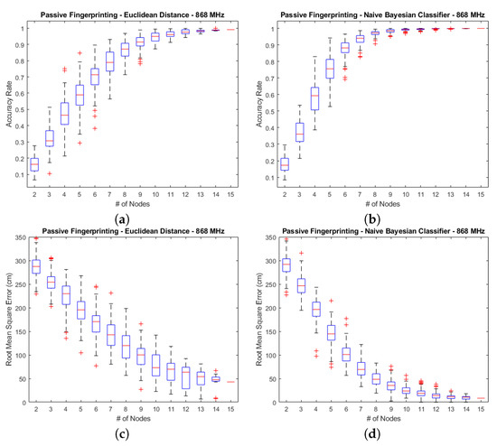
Figure 6.
Box plots of the accuracy rates and root mean square distance errors based on 868 MHz data. (a) and (b) show the accuracy rates for respectively the Euclidean distance-based and naive Bayesian classifier-based methods, while (c) and (d) show the root mean square distance errors for both approaches.
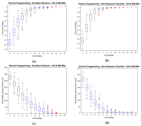
Figure 7.
Box plots of the accuracy rates and root mean square distance errors based on a combination of 433 MHz and 868 MHz data. (a) and (b) show the accuracy rates for respectively the Euclidean distance-based and naive Bayesian classifier-based methods, while (c) and (d) show the root mean square distance errors for both approaches.
Several conclusions can be derived from these results regarding the impact of the number of nodes, the frequency bands and the specific classification technique that were used.
First of all, the intuitive notion that lowering the number of nodes will generally cause the accuracy rate to decrease and the RMSE to increase seems to hold true. However, this is not a certainty. The precise locations of the nodes can have a significant impact on the resulting localization accuracy. To give an example, the worst combination of node positions for five nodes, on the 868 MHz frequency band and using the naive Bayesian method led to an accuracy rate of 0.53, while for the best combination this was equal to 0.94. When looking at the actual selected node combinations to obtain these specific rates as shown in Figure 8a,b, this large difference is quite evident. Figure 8a clearly shows a node selection which is concentrated on one side of the environment which leads to many potential locations which are far removed from any communication link. If a target is present in this part of the environment, the system does not have access to relevant RSS data to correctly estimate its location.
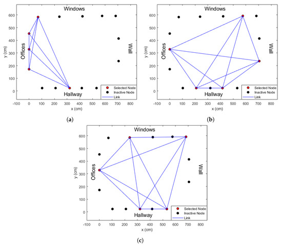
Figure 8.
The selection of five nodes which led to accuracy rates of (a) 0.53; (b) 0.94; and (c) 0.81, using a naive Bayesian classifier on RSS data from the 868 MHz network.
Other differences can be much more difficult to explain. When selecting the nodes as shown in Figure 8c, the corresponding accuracy rate is 0.81. This is a difference of 0.13 when compared to our most optimal selection. For an actual real-life implementation of a localization system, this would be a significant decrease of the system accuracy. No immediately obvious explanation for this can be gleaned from the two-dimensional schematic overviews of the test environment as shown in Figure 8. However, we are currently looking at the effects of major positional changes, but due to small-scale fading even minor node displacements can lead to drastically different RF propagation which can therefore indirectly impact system accuracy.
This phenomenon is well known within the field of RF-based DFL and generally a best effort approach is used when determining node locations. One highly interesting approach regarding this issue was proposed by Bocca et al. in [22]. In order to improve the accuracy of their RTI approach, they used servo motors which enabled them to slightly change the position of each RF sensor node in their network. Through an iterative process in which node location adjustments were made and evaluated, they managed to reduce localization errors in multiple environments by 32 % on average.
A second conclusion is that the 433 MHz measurements seem to be capable of slightly outperforming those of the 868 MHz frequency band. This can be seen by comparing the maxima of the corresponding box plots from Figure 5 and Figure 6. If we look at existing research within the literature, passive fingerprinting experiments performed by Xu et al. [16] seemed to echo these results with the use of 433.1 MHz leading to more accurate results than with the 909.1 MHz band in a 40 m bedroom environment. It was hypothesized that the presence of human motion caused smoother RSS variations for 433 MHz signals due to its larger wavelength and that this explained the increases in accuracy.
The best results are obtained as a result of combining the two frequencies, however. The additional RSS data provided to the algorithm by combining these two sub-GHz frequencies consistently leads to more accurate localization. Using only four nodes, the naive Bayesian classifier becomes capable of obtaining a root mean square error of only 48 cm. In our earlier DFL-research, which was on the topic of Radio Tomographic Imaging, a combination of these two frequencies proved to be superior to a single-frequency system as well [23].
It should be noted that these results cannot just be generalized for all DFL systems and the optimal choice of frequency band can depend heavily on the environmental context. For example, while 2.4 GHz is commonly used due to the fact that it is close to the resonance frequency of water and will therefore be strongly attenuated by the human body, it is difficult to deploy in very large environments due to its limited range. Additionally, its through-wall capabilities are limited when compared to lower frequencies and in very complex environments it might be too sensitive to multipath effects. On the other hand, sub-GHz frequencies are impacted less by human presence which can prove to be difficult for DFL as well.
Finally, the results also show the superiority of the naive Bayesian classifier when compared to the Euclidean distance. This was in line with expectations, as the performance of the Euclidean distance-based approach has consistently been rather poor within the state of the art [12,16] and it is often only used as a baseline to compare other techniques to.
In our next step, we will look at our results a little more in depth and investigate whether there are any differences if we look separately at the localization accuracy for each human target. Table 3, Table 4 and Table 5 show the accuracy rates of the median node selections for all frequencies and for each of the six participants when using the naive Bayesian classifier.
Table 3.
Median accuracy rates obtained by using a naive Bayesian classifier on data from the 433 MHz network.
Table 4.
Median accuracy rates obtained by using a naive Bayesian classifier on data from the 868 MHz network.
Table 5.
Median accuracy rates obtained by using a naive Bayesian classifier on data from both the 433 MHz and 868 MHz network.
We compare the results between these three tables and look at the differences based on the frequency bands that were used. Accuracy rates for 433 MHz and 868 MHz differ only slightly from each other and significant improvements are obtained by combining the two. This seems to be the case for all evaluation participants. If we compare the median accuracy rates from the different participants, however, we do notice an interesting pattern. The worst accuracy rates are consistently obtained by Participants 1, 5 and 6, regardless of the frequency band or the number of nodes. The differences between these three participants and numbers 2, 3 and 4 are often higher than 0.10 or even 0.15. Only in 2-node cases and cases in which the accuracy rates begin to approach values above 0.90 are these differences more minor. Additionally, it can also be seen quite clearly in the tables that participants 2, 3, and 4 require fewer nodes to obtain a perfect median accuracy rate of 1.
Potential reasons for these differences could lie in the fact that no training measurements for participants 5 and 6 were used in the construction of the fingerprint database. Additionally, participants 1 and 5 respectively have the lowest and second lowest height and weight out of all the participants. This is a clear indication that different individuals can have different impacts on a purely RSS based DFL system.
3.2. Constructing Separate Fingerprinting Databases for Each Training Participant
In our next step, we take a look at what happens if we only use training measurements from a single participant to construct the fingerprint database. We do so for the frequency band which has led to our most promising results thus far—a combination of 433 MHz and 868 MHz. Figure 9 shows the resulting accuracy rate box plots for both the Euclidean and naive Bayesian approaches if we use data from participant 1 to construct the database and evaluate based on data from all participants, including the training participant.
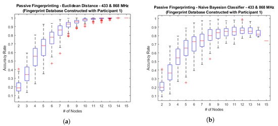
Figure 9.
Accuracy rates obtained for both the (a) Euclidean and (b) Bayesian methods on a combination of 433 MHz and 868 MHz RSS data, when only data from participant 1 was used for training.
It immediately becomes clear that—contrary to what hitherto had been the case—the naive Bayesian classifier actually performs worse than the Euclidean approach. In fact, the use of all 15 nodes no longer leads to a perfect accuracy rate but instead returns a rate of only 0.74 %. This could suggest that some level of overfitting occurs for the singular individual and the random stationary movements they made while the training measurements were performed. Interestingly, this leads to a situation in which the removal of a node leads to an unequivocal increase of the accuracy rate, regardless of which node is actually removed. While the results of the Euclidean approach are much more in line with what we saw earlier, the accuracy still shows a marked decline when compared to Figure 7a for which the training data from all participants was used.
We look into these results more deeply and investigate the median accuracy rates for each combination of training participant and evaluation participant. We do so for both 15 nodes and 7 nodes. The 7-node case was selected because, based on the results shown in Figure 5, Figure 6 and Figure 7, this was the least number of nodes for which a median accuracy rate above 90 % could still be obtained for both Bayesian and Euclidean approaches. Results are shown in Table 6, Table 7, Table 8 and Table 9.
Table 6.
Accuracy rates for each combination of training and evaluation participants. Results were obtained through the use of Euclidean distance minimization on RSS data from a 15-node 433 and 868 MHz network.
Table 7.
Accuracy rates for each combination of training and evaluation participants. Results were obtained through the use of a naive Bayesian classifier on RSS data from a 15-node 433 and 868 MHz network.
Table 8.
Median accuracy rates for each combination of training and evaluation participants. Results were obtained through the use of Euclidean distance minimization on RSS data from a 7-node 433 and 868 MHz network.
Table 9.
Median accuracy rates for each combination of training and evaluation participants. Results were obtained through the use of a naive Bayesian classifier on RSS data from a 7-node 433 and 868 MHz network.
For the 15-node Bayesian case, the use of the training data from participant 2 clearly leads to the most optimal results while the poorest accuracies are obtained with participant 1 training. In general, the highest accuracy rates for a given training participant are obtained if the same participant was also used for evaluation, but—with the exception of participant 2—these are still not equal to 1. This implies that the problem is not just a matter of overfitting to a specific participant but to a specific set of training measurements. After all, these results in combination with Figure 7b show that the accuracy rate when locating a specific participant improves when training data from other participants is added to the fingerprint database. We will discuss this in more detail in Section 5.
Similar remarks can be made for the 7-node Bayesian case. Training with participant 2 still seems to lead to the best results, with the exception of evaluating for participant 5. Additionally, while the Euclidean median accuracy rates are no longer equal to 1, they still tend to outperform their Bayesian equivalents. Interestingly, the Euclidean accuracies do not match the patterns of the Bayesian accuracies at all and participants 3 and 4 appear to be the most suitable candidates for training, rather than 2. One aspect which the results from both methods do appear to have in common, however, is the fact that in regards to evaluation, participants 1, 5 and 6 have the lowest accuracy rates. This could potentially be related to the low weight and height of participants 1 and 5, but this is not the case for participant 6. It should be noted, however, that amongst these three participants, 6 does usually have the highest accuracy rates. Further research regarding this aspect is required and we will discuss this in more detail in Section 5 as well.
4. Sub-GHz Passive Identification
In the previous section we have observed that the choice of participant(s) for both training and evaluation could have a significant impact on the localization accuracy. We will now investigate whether the different impacts of different participants can be used to distinguish between them. Instead of creating a single fingerprinting database with different entries for different locations, we create a separate database for each location with each entry corresponding to one of the four training participants. We assume that the location of the target is known, as the previous section has shown how trivial it is to obtain an accuracy of 100 % with 15 nodes if training data from multiple individuals is used. We randomly select 25 measurement vectors from each evaluation participant dataset and then construct confusion matrices for each location. Finally, we combine these confusion matrices into one large matrix representing the identification accuracy for the entire environment. Additionally, we present the accuracy rates for each location. Due to the fact that no training measurements exist for them, results for participants 5 and 6—while still shown in the confusion matrices—are not taken into account when calculating these accuracy rates.
All of the steps described in the preceding paragraph are performed for 433 MHz, 868 MHz and the two frequency bands combined, using both the Bayesian and Euclidean methods. Table 10 shows the total confusion matrix for the Euclidean method used on 433 MHz data and in Table 11 the same results can be found for the Bayesian approach. For both methods, the total confusion matrix was created by the summation of the separate confusion matrices for each location. Based on these confusion matrices, the accuracy rates for each location were calculated. These are shown in Figure 10a,b.
Table 10.
Confusion matrix for identification based on an Euclidean distance minimization approach applied to RSS data from the 433 MHz network.
Table 11.
Confusion matrix for identification based on a naive Bayesian classifier approach applied to RSS data from the 433 MHz network.
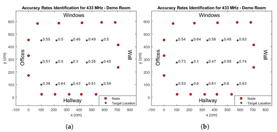
Figure 10.
Identification accuracy rates for each location for both the (a) Euclidean distance minimization and (b) naive Bayesian classifier approach applied to 433 MHz RSS data.
Table 12 and Table 13 and the corresponding Figure 11a,b show the same results for 868 MHz data. Finally, Table 14 and Table 15 and Figure 12a,b show this for a combination of both frequencies as well.
Table 12.
Confusion matrix for identification based on an Euclidean distance minimization approach applied to RSS data from the 868 MHz network.
Table 13.
Confusion matrix for identification based on a naive Bayesian classifier approach applied to RSS data from the 868 MHz network.
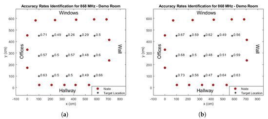
Figure 11.
Identification accuracy rates for each location for both the (a) Euclidean distance minimization and (b) naive Bayesian classifier approach applied to 868 MHz RSS data.
Table 14.
Confusion matrix for identification based on an Euclidean distance minimization approach applied to RSS data from both the 433 MHz and 868 MHz network.
Table 15.
Confusion matrix for identification based on a naive Bayesian classifier approach applied to RSS data from both the 433 MHz and 868 MHz network.
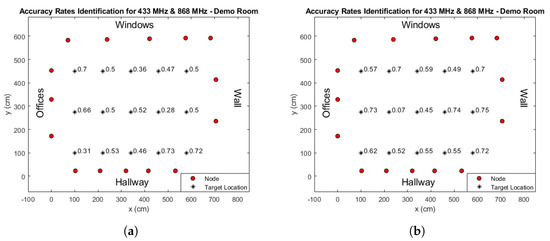
Figure 12.
Identification accuracy rates for each location for both the (a) Euclidean distance minimization and (b) naive Bayesian classifier approach applied to 433 MHz and 868 MHz RSS data.
We can derive many conclusions from these results. First of all, the identification results for most participants tend to be very poor, with the important exception of participant 1. Depending on the selected frequency and fingerprinting approach, the rate with which this participant is correctly identified varies between 0.93 and 1. This stands in stark contrast to the other participants, whose accuracy rates vary respectively between 0.10 and 0.62, 0.13 and 0.42 and 0.48 and 0.85 for participants 2, 3 and 4.
A potential explanation for this result could be the small weight and height of participant 1 as provided in Table 1. The differences in body type compared to the other participants could lead to such vastly different impacts on the RSS measurements that it becomes very easy to differentiate them. Indeed, whether or not differences in body type can lead to differentiation between individuals within an RSS-based passive fingerprinting system is one of the main questions driving this research. Now that we can answer this question in the affirmative based on this result, the next step consists of investigating how large differences in body type need to be in order to enable this differentiation. The only previously existing RSS-based passive identification study is—to the best of our knowledge—by Scholz et al. [18] and made use of three whose body types were vastly different (a young child, a regularly sized woman and a tall man) and they only managed to obtain a total accuracy rate of 0.67. Additionally, it should be noted that our confusion matrices indicate that whenever data from participant 5 was used, it was only very rarely estimated to be participant 1, despite the fact that their weight and height were closest when compared to all the other participants. While the very accuracy with which participant 1 can be differentiated from the other individuals is an encouraging step in the right direction, we do believe that there is much more research that needs to be performed and we will discuss this in the next section.
Second, in contrast to localization, it appears that the combination of data from two frequency bands does not seem to have any significantly positive effects in regards to identification accuracy. The total accuracy rates for 433 MHz, 868 MHz and the two of them combined are provided in Table 16 where this can clearly be seen. Only for the Euclidean approach does the frequency band have a minor impact on the total identification accuracy rates: 0.47 for 433 MHz, 0.52 for 868 MHz and 0.52 as well for a combination of the two. For the Bayesian method, the total identification accuracy rate is 0.58 regardless of frequency.
Table 16.
Overview of total identification accuracy rates for the entire experimental environment.
Finally, in the schematic overview images shown in Figure 10, Figure 11 and Figure 12 we can see that differences in accuracy rate between different locations are truly vast. As an example, the rates vary between 0.07 and 0.75 for the Bayesian approach using 433 MHz and 868 MHz data. A potential explanation for this would be that certain links which are affected most strongly when a target is present in a specific location are much more sensitive to differences between individuals. Determining whether this is true and if so, developing a method to identify and make use of these links are interesting topics for future research.
5. Conclusions and Future Work
In this paper, we experimentally investigated the use of two RSS-based passive fingerprinting techniques for both localization and identification of stationary human targets: one technique based on Euclidean distance minimization and one based on a naive Bayesian classifier. In particular, we focused on the impact of the number of RF nodes, the use of (multiple) sub-GHz frequencies and the body types of the targets on the resulting accuracy rates.
For localization, the relationship between the number of nodes and the resulting localization accuracies tended to follow a known pattern within the broader field of DFL. While decreasing the number of nodes generally led to an increased localization error, this was not always the case as accuracy rates for the same number of nodes could differ significantly depending on node locations. In regards to frequency, we found the differences between the 433 MHz and the 868 MHz band to be quite minor, but combining data from both consistently led to strong improvements in accuracy. Finally, it was shown that the selection of different targets, both for training the fingerprint database and for evaluation, can have a significant impact on localization accuracy as well. When the data from only a single experiment participant was used, instead of from all four for whom training measurements existed, accuracy rates for the naive Bayesian classifier plummeted below those of the Euclidean approach.
For identification, the resulting accuracy rates tended to be rather poor. The participant with the lowest height and weight (respectively 159 cm and 55.6 kg) was a major exception to this, however, as they were correctly identified more than 90 % of the time regardless of the fingerprinting technique and (combination of) frequency band(s) that were used. Frequency band selection in general appeared to have little impact on the results, even if 433 MHz and 868 MHz were combined. We also looked at the identification accuracies separately for each location and found that they could vary significantly from each other. When using the Bayesian classifier approach on 433 MHz data, one location had an identification accuracy rate rate of 0.1 while another location had one of 0.83.
While we could provide clear answers to our research questions regarding the number of nodes and the use of multiple sub-GHz frequencies in the context of passive fingerprinting-based localization, it is evident that a significant amount of future research needs to be performed in regards to the impact of the body type of a target and passive identification in general. The results provided in this study indicate that some level of differentiation is possible for body type categories that are far apart—in our case, participant 1 versus the other participants. This immediately invites follow-up questions regarding how these categories can be defined and how far apart they need to be from each other. In order to be able to answer them, it will be highly important to investigate which changes in RSS measurements between individuals are actually caused by differences in body type and which are the result of other factors (e.g., the random stationary movements performed by the participants during the training measurements described in this paper). This will require a vastly larger number of human participants compared to the experiments described within this paper. Furthermore, developing a method to identify the RF communication links which are most sensitive to body type differences will be crucial as well.
In addition to all of these aspects, much more advanced fingerprinting techniques will need to be investigated. Examples include random forest, support vector machine (SVM) and logistic regression classifiers which have all been used successfully in the context of 2.4 GHz passive radio mapping [15,17]. Furthermore, experiments will need to be performed in a variety of different environments, with targets that are not bound to static locations but move around freely. In particular, differences between environments regarding size and complexity (i.e., containing static objects) and the corresponding impact on classification accuracies will need to be thoroughly examined. Additionally, we will also need to look into the accuracy of the system if a target is not present in one of the exact fingerprinting locations. The relationship between this accuracy and the number of fingerprinting locations for different types of environments will be an important topic of research. Methods will need to be developed to take all of these aspects on both localization and identification into account.
Finally, we would like to note that RF-based device-free localization has become an increasingly popular topic of research [4] with a variety of potential applications [6,24,25]. In particular, the rise of the Internet-of-Things has led to significant interest in the use of “signals of opportunity” from already existing network infrastructure for DFL applications [26]. These types of systems would be very rapidly deployable, but it would not be possible to select the specific RF signals and node locations yourself. Therefore, in order to aid the further development of this field, there will be a need for public datasets from a variety of different environments, experimental setups and signals. The lack of public datasets is a major problem within the research field of RF-based DFL in general and we have previously discussed this in our earlier work [4]. Additionally, in the context of large-scale device-free crowd estimation, we have published one such dataset ourselves [27]. To lead by example, the data which was collected during the experiments described in this paper can be found through the link provided in the header of this paper. This dataset is accompanied by a small example in MATLAB code.
Author Contributions
Conceptualization, S.D.; Data curation, S.D. and A.K.; Formal analysis, S.D.; Investigation, S.D.; Methodology, A.K.; Software, S.D. and A.K.; Supervision, R.B. and M.W.; Writing—original draft, S.D.; Writing—review & editing, R.B. and M.W. All authors have read and agreed to the published version of the manuscript.
Funding
This research received no external funding.
Conflicts of Interest
The authors declare no conflict of interest.
References
- Patel, S.N.; Reynolds, M.S.; Abowd, G.D. Detecting human movement by differential air pressure sensing in HVAC system ductwork: An exploration in infrastructure mediated sensing. In International Conference on Pervasive Computing; Springer: Berlin/Heidelberg, Germany, 2008; pp. 1–18. [Google Scholar]
- Kashimoto, Y.; Fujimoto, M.; Suwa, H.; Arakawa, Y.; Yasumoto, K. Floor vibration type estimation with piezo sensor toward indoor positioning system. In Proceedings of the Indoor Positioning and Indoor Navigation (IPIN), 2016 International Conference on, IEEE, Madrid, Spain, 4–7 October 2016; pp. 1–6. [Google Scholar]
- Youssef, M.; Mah, M.; Agrawala, A. Challenges: Device-free passive localization for wireless environments. In Proceedings of the 13th annual ACM international conference on Mobile computing and networking, ACM, Montréal, QC, Canada, 9–14 September 2007; pp. 222–229. [Google Scholar]
- Denis, S.; Berkvens, R.; Weyn, M. A survey on detection, tracking and identification in radio frequency-based device-free localization. Sensors 2019, 19, 5329. [Google Scholar] [CrossRef] [PubMed]
- Yang, Z.; Zhou, Z.; Liu, Y. From RSSI to CSI: Indoor localization via channel response. ACM Comput. Surv. (CSUR) 2013, 46, 25. [Google Scholar] [CrossRef]
- Zou, H.; Zhou, Y.; Yang, J.; Spanos, C.J. Device-free occupancy detection and crowd counting in smart buildings with WiFi-enabled IoT. Energy Build. 2018, 174, 309–322. [Google Scholar] [CrossRef]
- Zeng, Y.; Pathak, P.H.; Mohapatra, P. WiWho: Wifi-based person identification in smart spaces. In Proceedings of the 15th International Conference on Information Processing in Sensor Networks, IEEE, Vienna, Austria, 11–14 April 2016; p. 4. [Google Scholar]
- Xin, T.; Guo, B.; Wang, Z.; Li, M.; Yu, Z.; Zhou, X. Freesense: Indoor human identification with Wi-Fi signals. In Proceedings of the 2016 IEEE Global Communications Conference (GLOBECOM), IEEE, Washington, DC, USA, 4–8 December 2016; pp. 1–7. [Google Scholar]
- Lv, J.; Yang, W.; Man, D.; Du, X.; Yu, M.; Guizani, M. Wii: Device-Free Passive Identity Identification via WiFi Signals. In Proceedings of the GLOBECOM 2017–2017 IEEE Global Communications Conference, IEEE, Singapore, 4–8 December 2017; pp. 1–6. [Google Scholar]
- Al-Husseiny, A.; Patwari, N. Unsupervised Learning of Signal Strength Models for Device-Free Localization. In Proceedings of the 2019 IEEE 20th International Symposium on “A World of Wireless, Mobile and Multimedia Networks” (WoWMoM), IEEE, Washington, DC, USA, 10–12 June 2019; pp. 1–9. [Google Scholar]
- Tan, J.; Guo, X.; Zhao, X.; Wang, G. Efficient Recognition of Informative Measurement in the RF-Based Device-Free Localization. Sensors 2019, 19, 1219. [Google Scholar] [CrossRef] [PubMed]
- Seifeldin, M.; Saeed, A.; Kosba, A.E.; El-Keyi, A.; Youssef, M. Nuzzer: A large-scale device-free passive localization system for wireless environments. IEEE Trans. Mob. Comput. 2013, 12, 1321–1334. [Google Scholar] [CrossRef]
- Xu, C.; Firner, B.; Moore, R.S.; Zhang, Y.; Trappe, W.; Howard, R.; Zhang, F.; An, N. SCPL: Indoor device-free multi-subject counting and localization using radio signal strength. In Proceedings of the 12th International Conference on Information Processing in Sensor Networks; ACM: New York, NY, USA, 2013; pp. 79–90. [Google Scholar]
- Sabek, I.; Youssef, M.; Vasilakos, A.V. ACE: An accurate and efficient multi-entity device-free WLAN localization system. IEEE Trans. Mob. Comput. 2015, 14, 261–273. [Google Scholar] [CrossRef]
- Mager, B.; Lundrigan, P.; Patwari, N. Fingerprint-based device-free localization performance in changing environments. IEEE J. Sel. Areas Commun. 2015, 33, 2429–2438. [Google Scholar] [CrossRef]
- Xu, C.; Firner, B.; Zhang, Y.; Howard, R.; Li, J.; Lin, X. Improving RF-based device-free passive localization in cluttered indoor environments through probabilistic classification methods. In Proceedings of the 11th International Conference on Information Processing in Sensor Networks; ACM: New York, NY, USA, 2012; pp. 209–220. [Google Scholar]
- Lei, Q.; Zhang, H.; Sun, H.; Tang, L. Fingerprint-Based Device-Free Localization in Changing Environments Using Enhanced Channel Selection and Logistic Regression. IEEE Access 2018, 6, 2569–2577. [Google Scholar] [CrossRef]
- Scholz, M.; Kohout, L.; Horne, M.; Budde, M.; Beigl, M.; Youssef, M.A. Device-free radio-based low overhead identification of subject classes. In Proceedings of the 2nd workshop on Workshop on Physical Analytics, Florence, Italy, 19 May 2015; pp. 1–6. [Google Scholar]
- Weyn, M.; Ergeerts, G.; Berkvens, R.; Wojciechowski, B.; Tabakov, Y. DASH7 alliance protocol 1.0: Low-power, mid-range sensor and actuator communication. In Proceedings of the Standards for Communications and Networking (CSCN), 2015 IEEE Conference on, IEEE, Tokyo, Japan, 28–30 October 2015; pp. 54–59. [Google Scholar]
- Maas, D.; Wilson, J.; Patwari, N. Toward a rapidly deployable radio tomographic imaging system for tactical operations. In Proceedings of the Local Computer Networks Workshops (LCN Workshops), 2013 IEEE 38th Conference on, IEEE, Sydney, Australia, 21–24 October 2013; pp. 203–210. [Google Scholar]
- Kaltiokallio, O.; Bocca, M.; Patwari, N. Follow@ grandma: Long-term device-free localization for residential monitoring. In Proceedings of the Local Computer Networks Workshops (LCN Workshops), 2012 IEEE 37th Conference on, IEEE, Clearwater Beach, FL, USA, 22–25 October 2012; pp. 991–998. [Google Scholar]
- Bocca, M.; Luong, A.; Patwari, N.; Schmid, T. Dial it in: Rotating RF sensors to enhance radio tomography. In Proceedings of the Sensing, Communication, and Networking (SECON), 2014 Eleventh Annual IEEE International Conference on, IEEE, Singapore, 30 June–3 July 2014; pp. 600–608. [Google Scholar]
- Denis, S.; Berkvens, R.; Ergeerts, G.; Bellekens, B.; Weyn, M. Combining multiple sub-1 ghz frequencies in radio tomographic imaging. In Proceedings of the 2016 International Conference on Indoor Positioning and Indoor Navigation (IPIN), IEEE, Madrid, Spain, 4–7 October 2016; pp. 1–8. [Google Scholar]
- Kianoush, S.; Savazzi, S.; Vicentini, F.; Rampa, V.; Giussani, M. Device-free RF human body fall detection and localization in industrial workplaces. IEEE Int. Things J. 2016, 4, 351–362. [Google Scholar] [CrossRef]
- Deak, G.; Curran, K.; Condell, J.; Asimakopoulou, E.; Bessis, N. IoTs (Internet of Things) and DfPL (Device-free Passive Localisation) in a disaster management scenario. Simul. Model. Pract. Theory 2013, 35, 86–96. [Google Scholar] [CrossRef]
- Savazzi, S.; Sigg, S.; Vicentini, F.; Kianoush, S.; Findling, R. On the Use of Stray Wireless Signals for Sensing: A Look Beyond 5G for the Next Generation of Industry. Computer 2019, 52, 25–36. [Google Scholar] [CrossRef]
- Kaya, A.; Denis, S.; Bellekens, B.; Weyn, M.; Berkvens, R. Large-Scale Dataset for Radio Frequency-Based Device-Free Crowd Estimation. Data 2020, 5, 52. [Google Scholar] [CrossRef]


© 2020 by the authors. Licensee MDPI, Basel, Switzerland. This article is an open access article distributed under the terms and conditions of the Creative Commons Attribution (CC BY) license (http://creativecommons.org/licenses/by/4.0/).