Article

Study of Deformation and Breakup of Submillimeter Droplets’ Spray in a Supersonic Nozzle Flow

Institute of Thermophysics Siberian Branch, Russian Academy of Sciences, Lavrentiev Ave 1, 630090 Novosibirsk, Russia
*
Author to whom correspondence should be addressed.
Appl. Sci. 2020, 10(18), 6149; https://doi.org/10.3390/app10186149
Submission received: 30 July 2020 / Revised: 27 August 2020 / Accepted: 31 August 2020 / Published: 4 September 2020
(This article belongs to the Special Issue Heat and Mass Transfer in Intense Liquid Evaporation)

Abstract

:
The problem of secondary atomization of droplets is crucial for many applications. In high-speed flows, fine atomization usually takes place, and the breakup of small droplets determines the final products of atomization. An experimental study of deformation and breakup of 15–60 µm size droplets in an accelerated flow inside a converging–diverging nozzle is considered in the paper. Particle image velocimetry and shadow photography were employed in the experiments. Results of gas and liquid phase flow measurements and visualization are presented and analyzed, including gas and droplets’ velocity, shape and size distributions of droplets. Weber numbers for droplets’ breakup are reported. For those small droplets at low Weber numbers, the presence of well-known droplets’ breakup morphology is confirmed, and rare “pulling” breakup mode is detected and qualitatively described. For the “pulling” breakup mode, a consideration, explaining its development in smaller droplets through shear stress effect, is provided.

1. Introduction

Experimental data on droplets behavior in high-speed flows is often required for such applications as combustion of liquid fuels, especially in ramjets, liquid atomization in airblast nozzles and many others. In general, the atomization of liquid droplets due to aerodynamic forces is a complex process that involves various physical mechanisms. Through the last several decades, a large number of experimental works aimed at revealing of influencing parameters, better understanding of breakup evolution and morphology, systematization of acquired data were performed.
A widely-adopted breakup morphology classification was proposed in the paper by Pilch and Erdman [1]. Since this publication, a lot of attention was paid to the physical phenomena, governing the droplets morphology and transition between regimes. Some of the results were summarized in the works by Gel’ fand [2] and Guildenbecher et al. [3]. The proposed classification was expanded, and the role of different phenomena was revised through a series of works summarized in the paper of Theofanous [4].
Generally, it is considered that Weber number (We), Ohnesorge number (Oh) and Eötvös or Bond number (Bo) govern the behavior of liquid drops in the flow, while an effect of Reynolds number (Re) is less apparent. The dimensionless parameters mentioned are expressed as:
W e = ρ g Δ v 2 d σ
B o = ρ d a d 2 σ
O h = μ d ρ d σ d
R e = ρ g Δ v d μ d
In these equations, ρg is the gas, Δv is the droplet-to-gas relative velocity, d is the initial droplet size (diameter), ρd, σ and µd are the density, surface tension and the dynamic viscosity of the liquid, respectively.
The Weber number is generally considered the most important parameter. In connection with the classification of breakup regimes introduced in [1], Weber number ranges are often referred to as “low”—We < 100, “medium” (100 < We < 350) and “high” (We > 350). Ohnesorge number expresses the measure of viscosity effect in breakup processes. Usually, transitional Weber numbers, demarking the breakup regimes, are considered stable for Oh < 0.1, while for a higher Oh increase in transitional We are typically observed (see [5]). At low Ohnesorge numbers, several breakup regimes are usually demarked according to We range: bag breakup for We > 12, multimode (multi-bag) or bag and stamen breakup for 30 < We < 80, sheet (or shear) stripping regime in the range of 80 < We < 350 and catastrophic regime at We > 350.
A droplet flattening into the ellipsoid form precedes any breakup regime. Hsiang and Faeth [6] provided an approximation for the maximum deformation of a droplet.
d m a x _ c / d = ( 1 + 0.19 W e )
where dy_c is the major axis of the ellipse (flattened droplet). Hsiang and Faeth also found, that for low Oh, total breakup time almost does not vary over the wide range of We and may be approximated as
t b = 5 t *
where t* is a characteristic time of breakup initiation t*, proposed by Ranger and Nichols [7].
t * = d Δ v ( ρ d ρ g ) 1 / 2
Other approximations taking into account tb dependence on We for different breakup regimes were also provided in [1].
According to [3,8], and many other papers, an effect of viscous shear stress, and therefore, Reynolds number, plays no significant role in the transition between breakup regimes. Some numerical studies suggest that Re, although not governing the breakup mode, has an effect on the shape of the droplet during the breakup. For example, studies performed by Han, and Tryggvason [9,10], showed that the liquid film surface area is correlated with Re. A similar conclusion can be drawn from the numerical investigation by Kekesi et al. [11].
The most common approaches to the experimental study of liquid drops deformation and breakup processes can be roughly divided into two categories: shock-tube experiments and experiments in continuous flows. Shock-tubes provide supersonic flow speed and controllable conditions, though instant aerodynamic loads can alter the behavior of the droplets comparing to the gradual acceleration case. Shock-tube approach was adopted, for example, in the works [12,13], and many others. Experiments with droplets in the continuous flow often provide more close resemblance to the practical application cases but also introduce additional parameters and effects to consider [14,15,16]. For example, in the paper by Wierzba [14] experiments on the bag type breakup of 2.2–3.9 mm size droplets in the continuous flow at near-critical We were reported. The main aim was to accurately determine the critical conditions necessary to complete the bag breakup. The author reported that five significantly different modes of droplet deformation and breakup were observed within the range of 11 ~< We ~< 14. Wierzba concluded that breakup of droplets at nearly critical We is very sensitive to fluctuations of the flow conditions. Similarly, in the review [3], the authors concluded that the transition between breakup regimes is a continuous process, while a single transitional We is an over-simplification.
The paper by Liu and Reitz [15] covered many issues, including droplets trajectory prediction and droplets morphology at different stages of a breakup for the bag, shear stripping and catastrophic regimes. Through scaling down the size of the droplet from 200 µm to 70 µm while preserving We, the authors showed that similar bag breakup regime occurred in both cases. Interesting to note, that in [15] authors observed the bag breakup regime at We = 56, while multimode or bag and stamen regime is considered to occur at such We numbers.
The physical mechanisms behind the bag and multimode breakup regimes are still a matter of discussion that primarily provides two different explanations. The first one attributes the bag breakup purely to the aerodynamic effects, while the second assumes that the bag breakup occurs due to the initial disturbance of the flattened droplet’s surface, caused by Rayleigh–Taylor (RT) instability. The work by Theofanous et al. [17] showed, among other results, that the second theory neatly explains the transition from bag to multimode breakup.
In the majority of the papers, droplets of size about 1 mm and larger are considered (see, for example, reviews [2,3]). For such droplets, low and medium Weber numbers at normal ambient conditions are achieved only at low, strongly subsonic gas velocities. At the same time, droplets of smaller size, usually produced in a primary jet, liquid film or a large droplet breakup at the atomizer, are also subjected to considerable aerodynamic loads in high-speed flow. While relative gas and droplets’ velocity can be high, up to supersonic, the Weber number for small droplets remains in the moderate or low range, resulting in a combination of dimensionless parameters, significantly different from those observed in experiments with large droplets. Another aspect is the change of flow conditions—rapid acceleration of small droplets, as well as the rapid change of velocity and density in supersonic flow—may lead to multiple switching of the We number range associated with specific breakup modes.
Examples of works in which the breakup of small droplets in high-speed continuous flows is considered are few, some of those being [18,19]. In both works droplets in a converging–divergent nozzle were investigated. Other examples are [8,20], in which high-speed vaporizing droplets of the size of about 200 µm, injected into the cross-flow, were studied. The work by Sommerfeld [18] did not provide insight into the processes of droplets’ breakup. Still, it showed that the final size distribution, in general, conforms to the expected one, derived from the existing breakup models.
Results provided by Kim and Hermanson [19] and further developed in [21], showed that under supersonic and overheating conditions, droplets exhibit breakup stages and morphology in some aspects different from commonly adopted. In the work [19], authors investigated a dynamics, breakup and vaporization of single volatile (overheated) and non-volatile small droplets in the underexpanded jet at supersonic gas-to-droplets relative Mach numbers. Droplet’s maximum Weber number in this experiment varied from 200 to 280 for different liquids, covering We range, typically associated with sheet-stripping breakup regime. One of the important features of this experiment was that droplets’ We number varied significantly during acceleration in the air flow: in the initial acceleration region, We remained in the low range but quickly increased to the values of We > 100.
One of the main conclusions brought by the authors was that for different test liquids droplet breakup followed a similar pattern that included four subsequent stages: the initial deformation of the droplet, sheet stripping, ‘primary breakup’ and a catastrophic breakup. Although not mentioned by the authors, the primary breakup could arguably be regarded as the transition phase from sheet stripping to the catastrophic regime. Authors also noted that the We at which the mentioned breakup regimes occur are generally higher than those reported previously for shock-tube experiments, and the total breakup times are an order of magnitude shorter than would be expected in shock-tube flows for similar Weber numbers.
In the present paper, a study of dynamics and breakup of submillimeter droplets, resulting from the primary breakup of the liquid jet, in a flow accelerating from subsonic to supersonic speed in a converging–diverging nozzle is reported. The work is focused on the deformation and breakup of small droplets and related flow characteristics at different regions of the flow. The motivation for the work was to bridge the gap in the experimental data for small droplets behavior at low, near-critical We numbers in continuous accelerating flow.

2. Materials and Methods

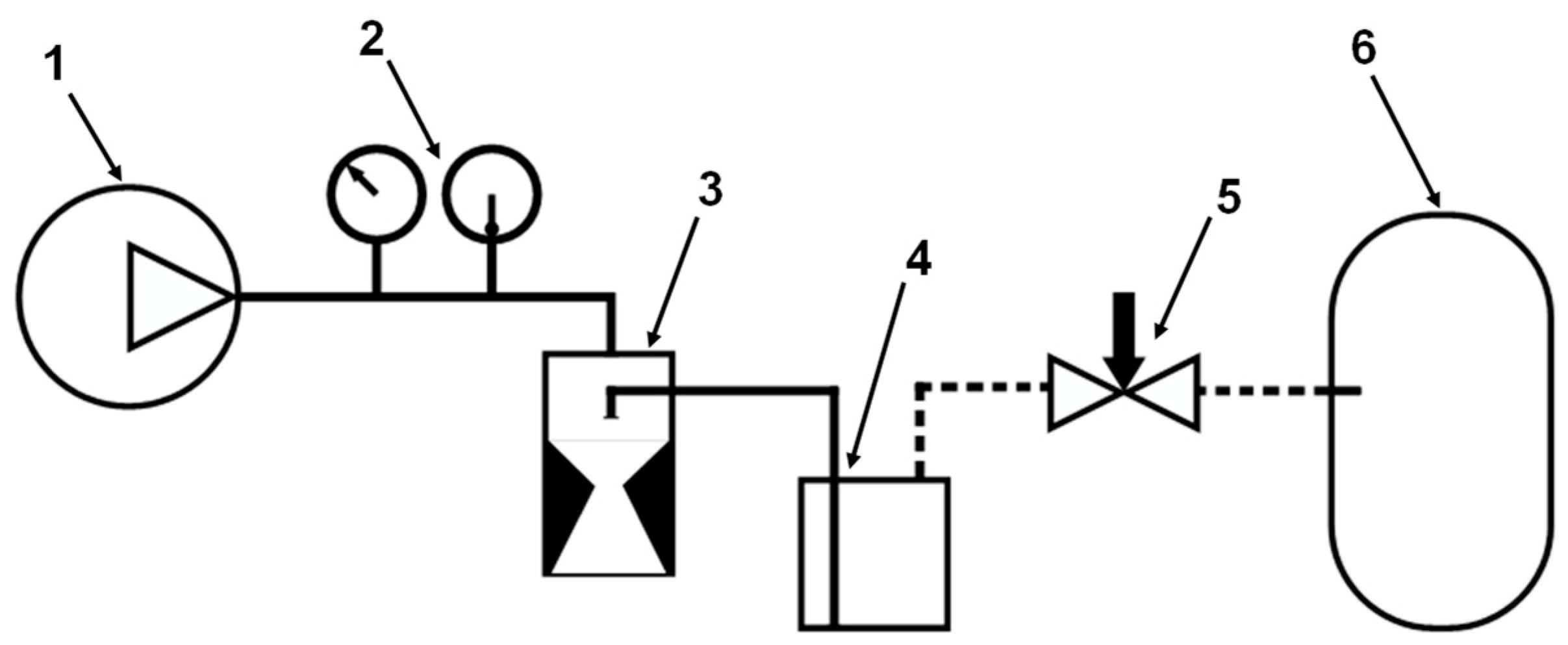
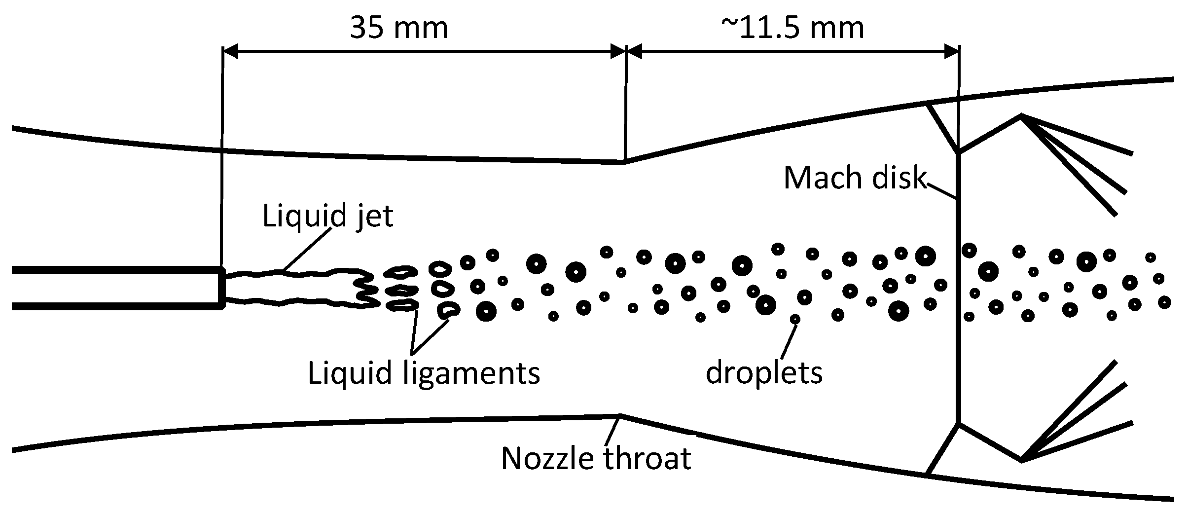
The behavior of liquid drops introduced into a gradually accelerating air flow in a converging–diverging nozzle was investigated. A converging–diverging nozzle with a rectangular cross-section and a throat size of 8 × 10 mm was employed for the study. Optical access to the measurement area was provided by transparent flat side walls of the nozzle. A compressor supplied constant airflow through the air supply line at the rate of 36 L/s. Air flow temperature and pressure were measured in the settling chamber preceding the converging part of the nozzle. The nozzle was operated in a choked regime with the formation of a Mach disk inside the divergent part of the nozzle, at a distance of 11.5 mm from the nozzle throat.
Droplets were introduced into the flow by atomization of the coaxial liquid jet of distilled water issued from the tube with an inner diameter of 0.5 mm. The exit of the tube was fixed in the settling chamber at a distance of 35 mm upstream of the nozzle throat. A fiber atomization regime of the round jet, described, e.g., in the review by Lasheras and Hopfinger [22], was observed at the exit of the tube. Large liquid clusters formed at the distance of 3–5 mm from the tube exit. Primary atomization was generally finished at the distance of 10–12 mm, the size of resulting drops mainly varied in the range from 10 to 100 µm. A scheme of the setup and the flow inside the nozzle is shown in Figure 1 and Figure 2, respectively.
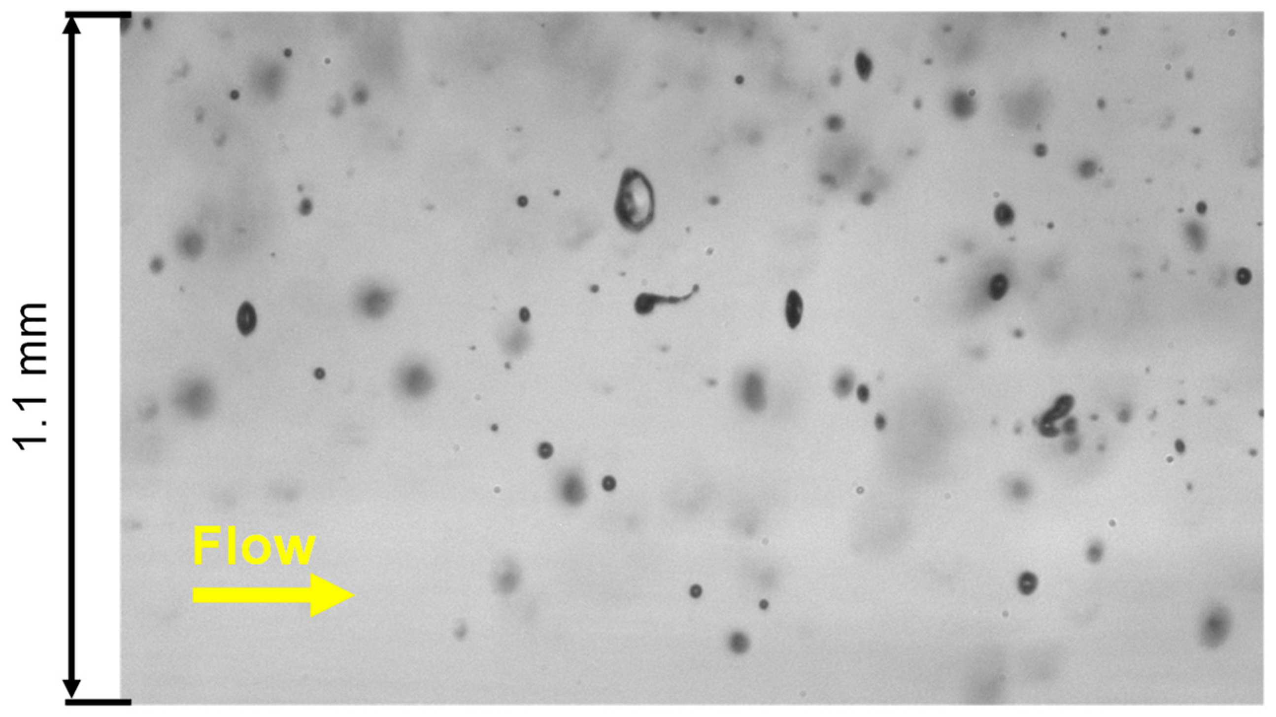
Direct visualization of droplet’s behavior in the flow using shadow photography (SP) played a key role in the work. To acquire a sharp image of a small-scale droplet in a supersonic flow, a high spatial resolution and short exposure are required. In the present work, short exposure was provided by a Rhodamine-B fluorescent background screen (thin cuvette filled with dyed ethanol), excited by 5–7 ns duration Nd:YAG laser (Quantel Evergreen EVG00200, Lannion, France) pulses. The fluorescent screen provided background lighting without speckles, which allowed visual analysis of small droplets. Images were captured by a CCD-camera (Bobcat B2020, Imperx, Boca Raton, FL, USA) with an Infinity K2/SC long-distance microscope (Infinity photo-optical, Centennial, CO, USA) with the optical magnification of 4.6:1, which is 1.6 µm/pix. An example of the SP image is shown in Figure 3.
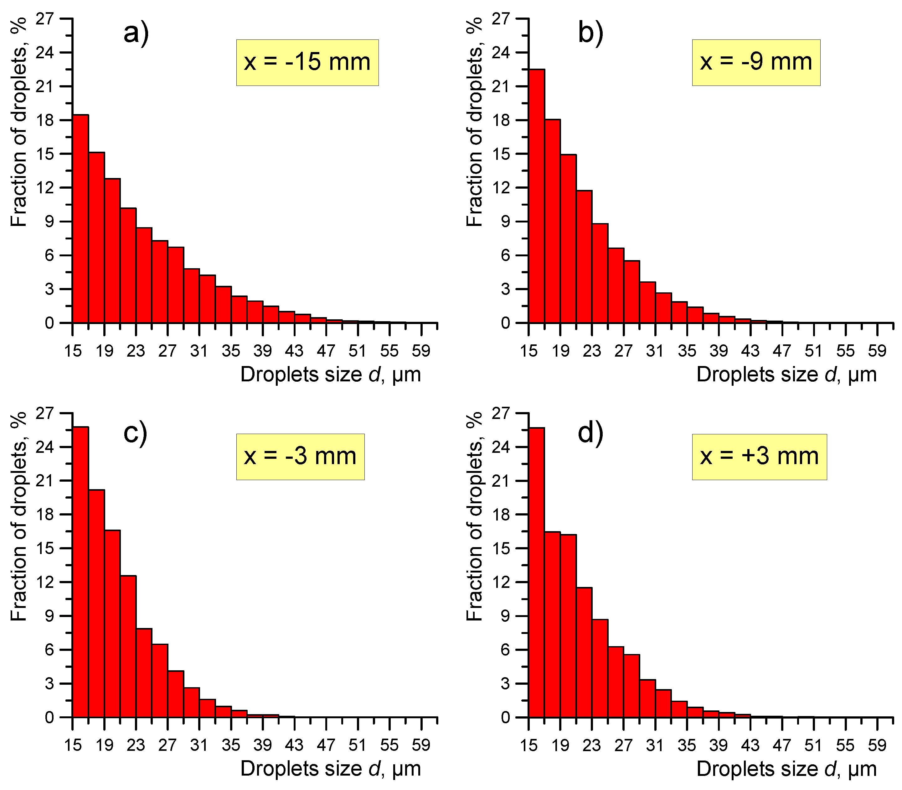
The spatial resolution of the images was enough to measure the size of droplets larger than 15 µm and to qualitatively analyze the morphology of droplets in the state of the breakup. At the same time, fine details and small droplets remained unresolved. An increase in spatial resolution could be useful for such tasks as the estimation of the breakup products’ size distribution and analysis of the droplets’ surface shape in the state of the breakup. An increase in resolution in future works can be achieved through the employment of cameras with smaller pixel size and employment of higher magnification optics, although considerations for the optics diffraction limit should be taken into account.
During the exposure time, droplets’ displacement was less than one pixel, and the motion blur of the droplets’ images was negligible. The use of a dual-head laser and a CCD-camera in double-frame exposure mode allowed capturing pairs of images with a short interframe delay (down to 300 ns), fetching not only instant images but also an evolution of the droplets over two frames. A small depth-of-field (DOF) of the microscope, which was about a few hundreds of micrometers, allowed to localize the measurement region in the central plane of the nozzle. At the same time, out-of-focus droplets significantly hindered the evaluation.
Automatic and manual processing of shadow images was employed for different purposes. Images of droplets in the state of the breakup were extracted and analyzed manually. Automatic processing was used to detect non-disrupting droplets in the images and to aggregate the statistical data for such droplets. The automatic image processing procedure was implemented using Python 3.6 programming language with Numpy 1.13.3 and OpenCV 3.3 open-source libraries. The processing procedure consisted of several steps. In the first step, a custom local variance filter [23] was applied to detect edges in the image. After that, a blob detector method from the OpenCV kit was employed to find contours (connected areas) in the image. The blob detector method performs multiple threshold binarization of images and extracts connected areas (contours) from each binary image using the border traversal algorithm implemented by the FindContours class of the OpenCV module. The blob detection procedure yielded a center of mass, the area and perimeter length of each detected contour. Variance filter and blob detector processing parameters were fine-tuned to detect only sharp contours of the droplets. No DOF correction method [24] was employed in the experiments, but, as the processing parameters were tuned specifically to reject even slightly blurred out-of-focus droplets, and the droplets’ size range was rather small, the statistical bias due to DOF effect could be ignored.
Additional filtering was applied to the extracted contours. Contours with the area smaller than 30 pixels2 (corresponding to the area of the droplet with equivalent sphere diameter d of 10 µm) were filtered out. Lower size threshold was set because smaller droplets were not expected to feature breakup or significant deformation.
The second filter employed the isoperimetric quotient Q of the contour as the parameter:
Q = 4 π S P 2
where S is the area of the contour, and P is the perimeter of the contour. Isoperimetric quotient shows a ratio of the contour’s area to the area of a circle with the same boundary length. Contours with Q < 0.6 were rejected. Such filtering passed elongated or slightly deformed droplets, but reliably rejected fibers, ligaments and droplets in the state of breakup. The filter with the threshold of Q = 0.6 passed the droplets with dmax/d < 1.8, considering a deformed droplet as an ellipse.
The processing method was tested on generated images and experimentally on the images of monodisperse glass microspheres (Whitehouse Scientific Ltd., Waverton, Cheshire, UK) of d = 25.6 µm and d = 84.3 µm, and yielded an RMS error of about 1.7 µm in the conditions similar to the present experiments.
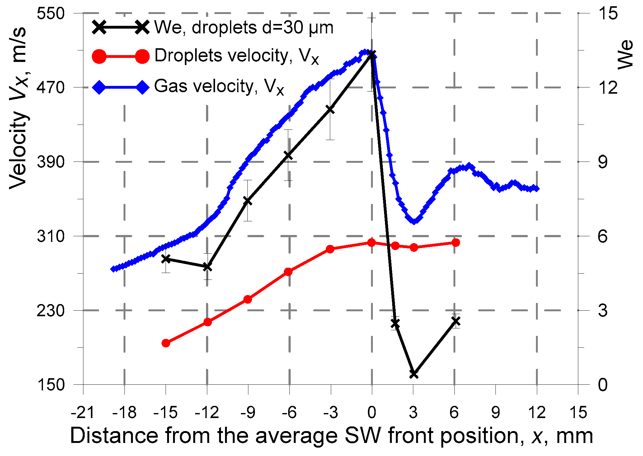
Additionally, particle image velocimetry (PIV) and particle tracking velocimetry (PTV) techniques were used to assess the gas and droplets’ velocity fields in the nozzle. Water-glycerol tracing particles of the size of about one µm were produced by the Laskin-nozzle type aerosol generator and were introduced into the air supply line immediately after the outlet of the compressor. Gas and droplets velocities were acquired in separate experiments. Gas velocity distribution was measured in the flow without droplets, as droplets’ images, which are much brighter than the images of tracer particles, made a proper evaluation of PIV data impossible. It is important to note for further consideration, that PIV tracer’s response to the abrupt deceleration of the flow after the shock wave front is not instant because of the tracer’s inertia. In the described experimental conditions. Relaxation length of the tracers after the shock wave (SW) front was about 2 mm, and the gas velocity data in this region were overestimated. A gas velocity distribution in a central plane of the nozzle is shown in Figure 4. Measured velocity pulsations near the axis of symmetry of the nozzle were in the range of ±2% of the mean gas velocity over the whole measurement area, excluding the region of ±1.5 mm from the average shock wave front position, within which a shock wave front oscillations occurred.
For the liquid phase (droplets), a PTV image processing algorithm was employed instead of PIV, as it was more suitable for measuring the average droplets’ velocity. In these measurements, no droplets’ size separation was made, and thus only average liquid phase velocity was measured. Gas and droplets’ velocity profiles are presented in 
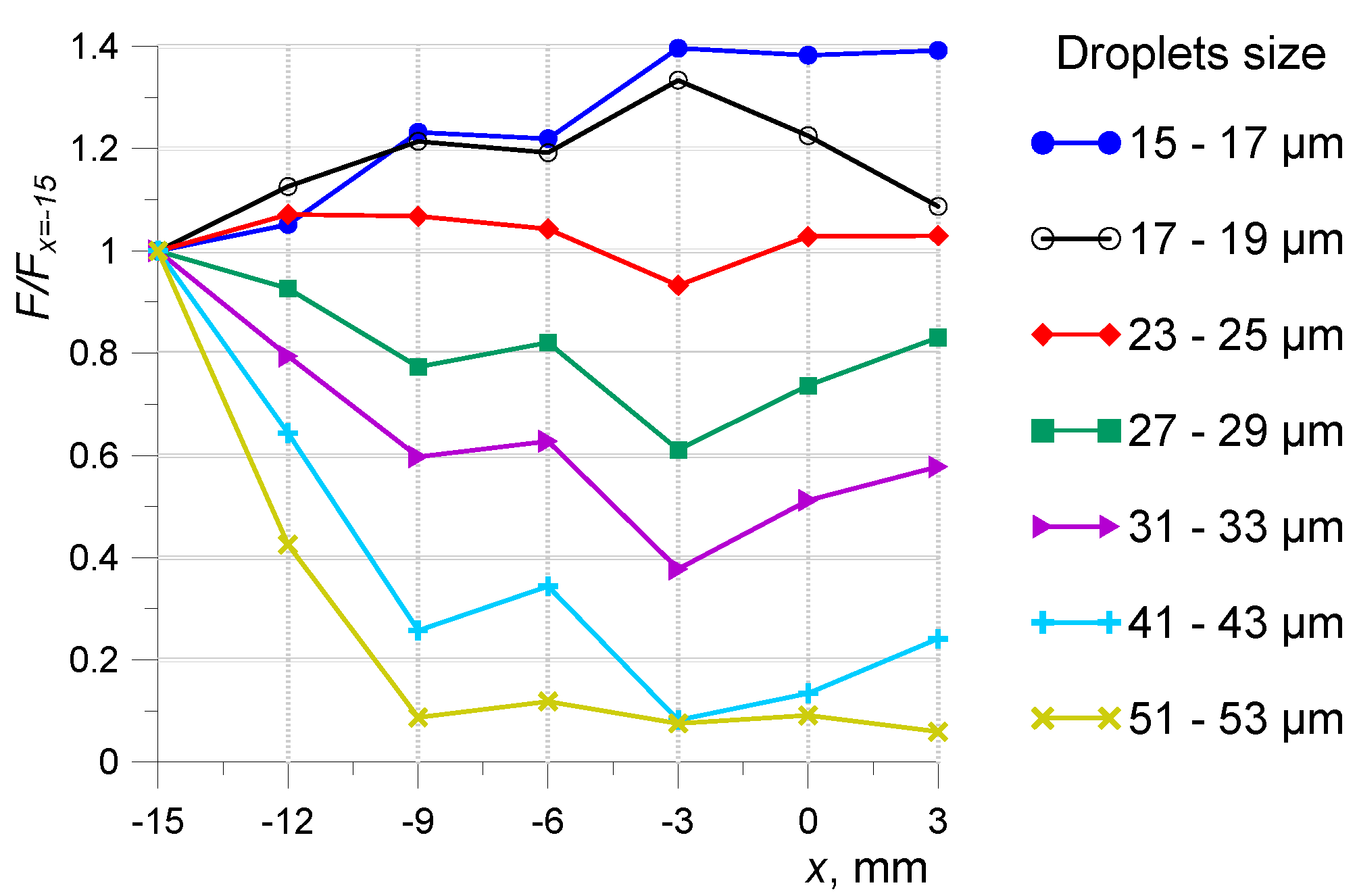
Figure 5. As droplets’ acceleration depends on their size, manual evaluation of velocity for droplets of different sizes in shadow images was performed. At the distance of 3 mm upstream of the average SW front position, the average velocity of 45 µm droplets was 275 m/s, while for 15 µm droplets, it amounted to 305 m/s. Therefore, an error introduced in the estimation of local We by neglecting the difference in velocity for droplets of different size was less than 10%.
As dimensionless parameters, including We, depend on the gas density, its variation along the nozzle should be taken into account. Initially, the gas density was evaluated through the isentropic gas flow equations at the point in the converging part of the nozzle, where pressure measurements were taken. After that, a density distribution along the axis of symmetry of the nozzle was estimated through the law of the mass flow rate conservation along the streamtube using density at the initial point and the gas velocity distribution from the PIV measurements. Error in density estimation was within ±6% of the value, considering the velocity measurement error and the precision of pressure and temperature sensors. Measured droplets and gas velocities combined with the evaluated gas density profile allowed to assess a Weber number variation along the axis of the nozzle with relative error within 11% of the value, assuming that the exact size of the droplet is known (Figure 5). As the droplets’ visualization region’s transverse size was quite small, about 3.5 mm, and was always centered at the axis of symmetry of the nozzle, the velocity and We data at the axis were used as a reference for all of the considerations about droplets behavior.

3. Results

3.1. Flow Configuration

As shown in Figure 4 and Figure 5, gas flow exhibits smooth acceleration with subsequent step deceleration at the SW front, which was located at the distance of approximately 11.5 mm downstream of the nozzle throat. From here on, the average SW front position is used as a reference point of x-axis (x = 0). The flow structure upstream of the SW front remained the same in general, yet oscillations of the SW front within the range of ±1.5 mm from its average position and variations of the velocity were observed. Such instability is most likely appeared due to non-stationary flow conditions downstream of the SW front. The maximum velocity immediately before the SW front varied approximately from 480 to 520 m/s.
Droplets exhibited smooth acceleration along the area upstream of the SW front, but significantly lagged behind the gas flow. As a result, droplets’ velocity in the vicinity of the SW front was close to the gas velocity downstream of it. Therefore, the impact of the aerodynamic forces on droplets decreased abruptly after the SW front. The relative droplets-to-gas velocity Δv did not exceed supersonic level, being in the range from 90 to 200 m/s.
In Table 1, dimensionless parameters affecting the droplets’ dynamics and breakup for various sizes of the droplets are presented, as well as the characteristic time of breakup induction t*.
One of the features of the experiment is the rapid change of gas velocity and density, which results in a high Weber number gradient. Droplet residence time in the area of accelerating supersonic flow is about 60 µs, which is comparable to the total breakup time provided by Equation (6), (tb ≈ 60 µs for the droplet diameter d = 30 µm). Droplets travel the distance of 10 mm while the droplets We doubles. This can lead to the switching of the breakup regime. Ohnesorge number for droplet sizes under consideration was far below the critical value of 0.1, above which Weber numbers, demarking breakup modes, tend to grow with an increase of Oh.

3.2. Droplets Size, Shape Oscillations, and Breakup

Over 600 pairs of shadow images with different interframe delay were acquired in the area from x = −15 mm (upstream) to x = +3 mm (downstream) with the distance of 3 mm between the centers of the visualization regions. The average size and shape of droplets were evaluated from shadow images (see Figure 6). Statics of about 1.5 × 10⁴ droplets were collected for each visualization region. Only droplets in size range of 15–60 µm that retained spherical or elliptical shape (up to dmax/d = 1.8) and did not exhibit breakup were taken into account. An average droplet’s size, that is an average diameter of a sphere of equal volume:
d = d x d y 2 3
where dx is a streamwise ellipse dimension and dy—transversal ellipse dimension, was in the range of 20–24 µm in the whole measurement area. Most of the droplets (from 95 to 99% in different regions) were in a range of sizes from 15 to 39 µm. The plots in Figure 6 show that the average droplet size <d> and size variance δd gradually drop along the axis until droplets reach the SW front position, indicating that larger droplets tend to break up. A small increase in <d> and δd immediately after the SW front is likely due to the coalescence of decelerating droplets. Although described variations are almost within the range of single droplet size random measurement error (about ±1.7 µm), for the ensemble-averaged data based on thousands of droplets, the error is essentially negligible.
The plot of the elongation defined as
e d = d m a x / d
indicates the intensity of the aerodynamic load and conforms to the Weber number profile (see Figure 5). Larger droplets exhibit a larger variance of the elongation δe (shown as error bars in the plot) and stronger deformation. Elongation of droplets appears to be insufficient for the transition to breakup if compared with the estimation provided by the Equation (5), which yields a critical elongation dmax_c of 1.6–1.65 for the transitional We of 10–12. At the same time, some of the droplets in the size range of 45–51 should be close to the transition to the breakup, taking into account the variance of the elongation. Data for the region located at x = −6 stands out in both plots shown in Figure 6, while there is no average velocity or We defect in this region. A possible explanation is the effect of the expansion fan (Prandtl–Meyer expansion) propagating from the nozzle throat and forming a diamond-shape pattern with leading waves intersection around x = −6. This pattern can be noticed in Vy velocity field in Figure 4. Thus, a noticed defect in the plot can be explained by the cease of action of expansion waves, such as wave drag, on droplets.
To get more detailed information on droplets evolution along the nozzle, a size distribution for each of the visualization regions was calculated. Size distribution was truncated for d < 15 because smaller droplets were poorly resolved, and were not expected to exhibit any breakup or substantial deformation. Distributions for some of the regions are presented in Figure 7 and the evolution of the fraction of droplets of different sizes over the regions—in Figure 8. In addition, more detailed information on the fraction of droplets over the different regions in the form of a table and additional figures, showing the evolution of the normalized droplets fraction F/Fx=−15, where Fx=−15 is droplet fraction at x = −15 mm, are provided in Appendix A (see Table A1 and Figure A1, respectively).
A fraction of droplets in size range of 15–23 µm gradually increased along the x-axis up to the SW front. Around the average position of the SW front and 3 mm downstream of it, the fraction of such droplets decreased due to coalescence. Such droplets did not exhibit breakup nor upstream nor downstream of the SW front. Wemax for such droplets is 9.6.
For the droplets in the size range of 23–27 µm, their fraction remained almost constant along the whole path of the spray. On the bases of this observation, a size of 27 µm (Wemax = 11.2) can be interpreted as a threshold for the droplets that do not disrupt. A We number of 10–12 is a classical value for the transition to bag breakup regime, reported in many papers [1,25]. This allows concluding that in described conditions, the main physical mechanisms governing the droplets’ breakup remain the same for small droplets.
A fraction of droplets of larger size decreased, reaching the minima at the distance of 3 mm downstream of the SW front. For larger droplets, the decrease was faster. A fraction of droplets with the size d > 50 µm (Wemax 22.2) was almost negligible. The total amount of such droplets was about 2% at the beginning of the measurement area (x = −15 mm) and fell to 0.1% at a distance of 3 mm downstream of the SW front. Due to a small number of such droplets, the evolution of normalized fraction for the droplets in this size range, shown in Figure A1 may be biased. Interesting to note that a slight decrease in the fraction of larger droplets starts at the beginning of the measurement area. In addition, despite exceeding the bag breakup regime We threshold, some of the larger droplets did not exhibit breakup or exhibited significantly delayed breakup least, as they persisted, although in small quantities, in the flow upstream and downstream of the SW front.
The observed trends for gradual increase and decrease of the fraction of droplets allow to suggest that empirical approximation can be derived to predict the evolution of droplets size distribution using the initial (measured at the single point or region) distribution and known gas flow parameters. Still, to achieve this goal, more data, statistics and validation cases for various experimental conditions are required.
Regarding the droplets’ morphology, most of the droplets observed in a state of disruption resembled bag breakup at different stages (Figure 9), described in [14,25]. Larger droplets tended to disrupt through dual-bag and multi-bag formations, described in [26]. For the bag breakup in many events, a collapse of an underdeveloped bag was noticed. In this case, instead of explosive bag disruption with the formation of a cloud of small drops, the bag used to collapse into several fibers attached to the rim or shrink to the deformed droplet shape (also shown in Figure 9). Currently, there is no developed theory that would fully describe a process of bag rupture. Arguably, initial bag rupture may be explained through instability growth at the thin liquid sheet separating two gaseous media [27]. Jalaal and Mehravara [28] performed a numerical simulation of the bag breakup of the droplet at different Bo numbers and connected the results with the mentioned assumption. They found that an increase in Bo results in a significantly larger number of ‘punctures’ in the bag surface at the onset of its rupture, which, in turn, results in a notable increase in the number of generated ligaments. In Figure 9, two expanding punctures in the bag can be seen in the first frame. In the experiments under consideration, the Bond number was relatively low, about 40 for droplets with d = 40 µm. Thus, a small number of ligaments produced in film rupture may be attributed to the low Bond number. Although the dominant presence of large ligaments can be explained in this way, small droplets should also be produced in bag breakup. In the current experiments, they were not resolved by the imaging system. Indeed, if the size of daughter droplets is comparable to the liquid film thickness, droplets of the size about d × 10−3 or smaller should be expected [29]. Numerical simulation performed by Jain et al. [30] has shown that in bag breakup regime, daughter droplets of about 1–4% of the initial droplet size are mainly produced. Even in this case, for initial droplets size about 40 µm, most of the daughter droplets should be about 0.8, which is two times smaller than a resolution of the imaging system.

3.3. “Pulling” Breakup

Another breakup morphology, many cases of which were observed in the flow, resembled so-called “pulling”, distinguished as a separate regime in [17] and noted in [19] as an early stage of breakup in underexpanded jet. This regime deserves a more detailed discussion, as little attention was paid to it earlier.
In case of pulling, a stamen emerges in the wake of a droplet, then grows into a long fiber and disrupts into a number of much smaller droplets with seemingly equal intervals between them, resembling round jet breakup in Rayleigh regime or, more likely in first wind-induced regime [31], which occurs at jet Weber numbers of 0.4 < Wej < 13. Wej is expressed similar to Equation (1), but with a jet diameter instead of the droplet size.
In some cases at an early stage, a liquid film begins to form, collapsing into a stem shortly after. The subsequent scenario does not differ from the pulling breakup scenario without initial film formation. Early liquid film formation may indicate the beginning of a competing bag breakup regime that switches to a pulling breakup. An illustration of pulling breakup stages, combined from several events, is shown in Figure 10.
The experimental technique allowed capturing only two subsequent images, which is not suitable for tracking the evolution of the droplet’s breakup. As a result, only snapshots of the pulling process could be detected in the captured breakup events. This leaves the nature of the observed pulling breakup somewhat unclear, though the most probable explanation, proposed in the paper [17], is a viscous drag that transports the liquid to the wake of the droplet due to the high shear stress.
Indeed, for the shear stress in the laminar boundary layer:
τ ~ μ υ d R e = μ σ Δ v d 2 W e
Thus, when scaling a droplet size by a factor of k, while preserving a Weber number, a shear stress value changes as k 5 / 4 v scales as k 1 / 2 to preserve We). Scaling a droplet size d from 1 mm down to 50 µm yields an increase in τ by a factor of ≈ 22. Note that in the experiments by Theofanous et al. [20], due to the conditions (highly rarefied flow, relative Mach number ≈ 3, large droplets), the increase in τ, estimated in the same manner, was about 4.2, which also supposedly led to a manifestation of the pulling regime.
A statistic of about 300 fully developed pulling events were extracted from images and analyzed. Droplets in pulling breakup state were mainly in the range of We from 4 to 14. The equivalent size of the droplet was calculated as:
d = 6 ( V b o d y + V s t e m ) π 3
where Vbody and Vstem are the volumes of the droplets body and the stem, respectively. A stem shape was approximated as a cylinder for this purpose, and the droplet’s body shape was approximated as a spheroid. A cumulative percentage of detected pulling breakup events against We is shown in Figure 11a. Few events were detected at the We above 14, but their presence is most likely can be attributed to the error in determining a We number for the droplet. Still, an overlap between bag breakup range and observed pulling breakup range exists at the Weber numbers of 11–14. This overlap is reasonable in the light of some previous works (see, for example, a reference to the paper by Wierzba [14] or Guildenbecher et al. [3] in the introductory section), claiming that transition between regimes is a continuous process, rather than a process with a single-value threshold.
The length of the stem tends to grow with an increase of the Re number and the size of the initial drop (see Figure 11). This result may support the assumption that the pulling breakup is caused mainly by the shear stress. A large spread of acquired data, however, makes it impossible to derive a reliable approximation for the named tendencies. A spread in data, at least partially, may be attributed to the fact that the stem length was measured at a developed state, but not necessarily at the moment of maximum extension.
It is important to note that only part of the droplets in the specified Weber number range used to disrupt via pulling regime. At the same time, no visible deformations in droplets before they transitioned to the pulling breakup (see an example of transition in Figure 12) could be noticed. This suggests that in addition to We, other possible influencing parameters, including external flow disturbances, should be considered in the future to explain the initiation of pulling breakup.

4. Conclusions

A behavior of submillimeter-scale water droplets produced by a liquid jet breakup in the flow in a converging–diverging nozzle was investigated using a set of optical techniques. Flow configuration, including gas velocity and density distributions, were evaluated from point-wise and planar measurements. Shadow photography allowed to specify velocity ranges for different droplet sizes and to visualize droplets dynamics and breakup modes.
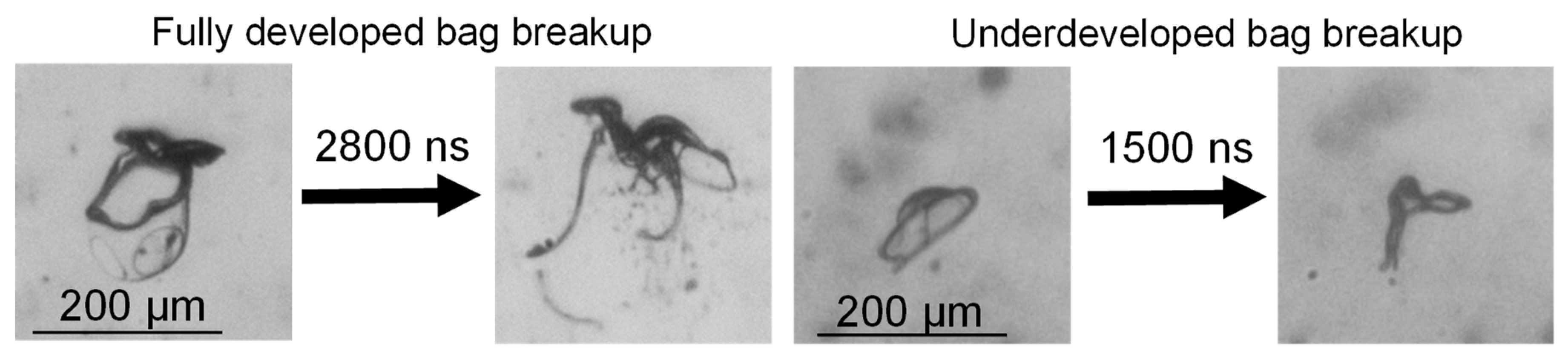
No evidence of systematic droplets’ breakup at the Weber numbers below 12 was detected, while for higher Weber numbers, the bag and multi-bag breakup regimes were dominant. In general, small-scale droplets in the range of low We numbers feature the same breakup processes and thus are governed by similar physical mechanisms, as large (size of a millimeter) droplets.
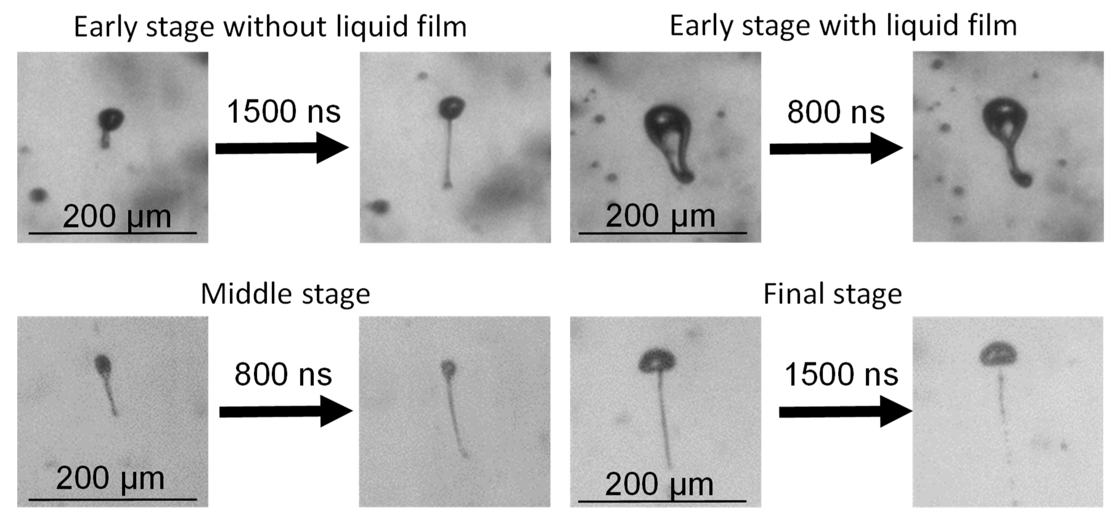
A qualitative description of pulling breakup regime, detected at low Weber numbers, ranging from 4 to 14, is given. In this regime, a stem emerges from a droplet, and smaller droplets are produced through disruption of the stem, presumably through fluid thread breakup. It was noted that the length of the stem has a positive correlation with the local Reynolds number (Re) and size of the initial drop. An additional consideration, explaining the manifestation of pulling breakup regime in smaller droplets through shear stress, is provided. The proposed explanation suggests that with a particular combination of flow parameters, shear stress can play a significant role in the atomization process.
The studies reported, and the results obtained are of certain practical importance. In the first place, they can be used to refine the methods and models for the prediction of final atomization products in applied problems.

Author Contributions

Investigation, O.A.G., M.N.R.; writing—original draft preparation, O.A.G., A.V.B.; writing—review and editing, O.A.G., A.V.B.; methodology—O.A.G., A.V.B.; supervision, A.V.B. All authors have read and approved the submitted version of the manuscript.

Funding

Research was funded by the Government of the Russian Federation, grant No. 075-15-2019-1888.

Acknowledgments

Government of the Russian Federation (grant No. 075-15-2019-1888).

Conflicts of Interest

The authors declare no conflict of interest.

Appendix A

Table A1. Fraction of droplets in the specified size range for different regions of the flow, %.
Coordinate−15 mm−12 mm−9 mm−6 mm−3 mm0 mm+3 mm
Size Range
15–17 µm18.4519.4122.7322.5025.7725.5225.69
17–19 µm15.1317.0418.3818.0420.1918.5416.45
19–21 µm12.7913.5715.4114.9116.5915.4116.21
21–23 µm10.1610.1511.2911.7412.5611.3511.51
23–25 µm8.449.049.018.807.878.688.69
25–27 µm7.297.456.786.646.496.596.27
27–29 µm6.716.225.195.514.104.945.58
29–31 µm4.794.793.783.632.623.043.34
31–33 µm4.233.362.532.661.602.172.44
33–35 µm3.232.901.801.860.971.471.43
35–37 µm2.371.851.141.400.611.030.90
37–39 µm1.931.320.730.860.230.550.55
39–41 µm1.470.980.440.570.210.340.42
41–43 µm1.010.650.260.350.080.140.24
43–45 µm0.740.420.180.200.020.070.08
45–47 µm0.460.320.140.150.020.090.08
47–49 µm0.250.200.070.060.020.040.03
49–51 µm0.180.150.070.040.000.010.05
51–53 µm0.160.070.010.020.010.010.01
53–55 µm0.090.050.030.040.000.010.02
55–57 µm0.060.040.000.020.040.000.01
57–59 µm0.020.010.010.010.000.000.00
59–61 µm0.030.020.030.000.010.000.00
Figure A1. Evolution of the normalized droplets’ fraction F/Fx=−15 along the centerline of the nozzle. For each coordinate, the fraction of droplets is normalized by the fraction of droplets in the same size range in the first visualization region at x = −15.
Applsci 10 06149 g0a1

References

  1. Pilch, M.; Erdman, C.A. Use of breakup time data and velocity history data to predict the maximum size of stable fragments for acceleration-induced breakup of liquid drop. Int. J. Multiph. Flow 1987, 13, 741–757. [Google Scholar] [CrossRef]
  2. Gelfand, B.E. Droplet breakup phenomena in flows with velocity lag. Prog. Energy Combust. Sci. 1996, 22, 201–265. [Google Scholar] [CrossRef]
  3. Guildenbecher, D.R.; López-Rivera, C.; Sojka, P.E. Secondary atomization. Exp. Fluids 2009, 46, 371–402. [Google Scholar] [CrossRef]
  4. Theofanous, T.G. Aerobreakup of newtonian and viscoelastic liquids. Annu. Rev. Fluid Mech. 2011, 43, 661–690. [Google Scholar] [CrossRef]
  5. Faeth, G.M.; Hsiang, L.P.; Wu, P.K. Structure and breakup properties of sprays. Int. J. Multiph. Flow 1995, 21, 99–127. [Google Scholar] [CrossRef]
  6. Hsiang, L.P.; Faeth, G.M. Near-limit drop deformation and secondary breakup. Int. J. Multiph. Flow 1992, 23, 635–652. [Google Scholar] [CrossRef] [Green Version]
  7. Nicholls, J.A.; Ranger, A.A. Aerodynamic shattering of liquid drops. AIAA J. 1969, 7, 285–290. [Google Scholar] [CrossRef]
  8. Liu, Z.; Reitz, R.D. An analysis of the distortion and breakup mechanisms of high speed liquid drops. Int. J. Multiph. Flow 1997, 23, 631–650. [Google Scholar] [CrossRef]
  9. Han, J.; Tryggvason, G. Secondary breakup of axisymmetric liquid drops. I. Acceleration by a constant body force. Phys. Fluids 1999, 11, 3650–3667. [Google Scholar] [CrossRef]
  10. Han, J.; Tryggvason, G. Secondary breakup of axisymmetric liquid drops. II. Impulsive acceleration. Phys. Fluids 2001, 13, 1554–1565. [Google Scholar] [CrossRef]
  11. Kekesi, T.; Amberg, G.; Wittberg, L.P. Drop deformation and breakup. Int. J. Multiph. Flow 2014, 66, 1–10. [Google Scholar] [CrossRef]
  12. Hinze, J.O. Fundamentals of the hydrodynamic mechanism of splitting in dispersion processes. AIChE J. 1955, 1, 289–295. [Google Scholar] [CrossRef]
  13. Joseph, D.D.; Bellanger, J.; Beavers, G.S. Breakup of a liquid drop suddenly exposed to a high-speed airstream. Int. J. Multiph. Flow 1999, 25, 1263–1303. [Google Scholar] [CrossRef]
  14. Wierzba, A. Deformation and Breakup of liquid drops in a gas stream at nearly critical Weber numbers. Exp. Fluids 1990, 9, 59–64. [Google Scholar] [CrossRef]
  15. Liu, A.B.; Reitz, R.D. Mechanisms of air-assisted liquid atomization. At. Sprays 1993, 3, 55–75. [Google Scholar] [CrossRef]
  16. Lee, C.H.; Reitz, R.D. An experimental study of the effect of gas density on the distortion and breakup mechanism of drops in high speed gas stream. Int. J. Multiph. Flow 2000, 26, 229–244. [Google Scholar] [CrossRef]
  17. Theofanous, T.G.; Li, G.J.; Dinh, T.N. Aerobreakup in rarefied supersonic gas flows. J. Fluids Eng. Trans. ASME 2004, 126, 516–527. [Google Scholar] [CrossRef]
  18. Sommerfeld, M.; Kurian, J. Droplet Behaviour in Underexpanded Supersonic Jets. In Proceedings of the 19th International Symposium on Shock Waves, Marseille University, Marseille, France, 26–30 July 1993; Brun, R., Dumitrescu, L.Z., Eds.; Springer: Berlin/Heidelberg, Germany, 1995. [Google Scholar]
  19. Kim, Y.; Hermanson, J.C. Breakup and vaporization of droplets under locally supersonic conditions. Phys. Fluids 2012, 24, 076102. [Google Scholar] [CrossRef]
  20. Hwang, S.S.; Liu, Z.; Reitz, R.D. Breakup mechanisms and drag coefficients of high-speed vaporizing liquid drops. At. Sprays 1996, 6, 353–376. [Google Scholar]
  21. Lin, E.P.; Kim, Y.E.; Hermanson, J.C. Structure of Compression Waves on Supersonic Droplets. AIAA J. 2016, 54, 774–778. [Google Scholar] [CrossRef]
  22. Lasheras, J.C.; Hopfinger, E.J. Liquid jet instability and atomization in a coaxial gas stream. Annu. Rev. Fluid Mech. 2000, 32, 275–308. [Google Scholar] [CrossRef]
  23. Fabijanska, A. Variance filter for edge detection and edge-based image segmentation. In Proceedings of the 2011 VIIth International Conference on Perspective Technologies and Methods in MEMS Design, Polyana, Ukraine, 11–14 May 2011; pp. 151–154. [Google Scholar]
  24. Kim, K.S.; Kim, S.S. Drop Sizing and Depth-of-Field Correction in TV Imaging. At. Sprays 1994, 4, 65–78. [Google Scholar] [CrossRef]
  25. Hsiang, L.P.; Faeth, G.M. Drop deformation and breakup due to shock wave and steady disturbances. Int. J. Multiph. Flow 1995, 21, 545–560. [Google Scholar] [CrossRef] [Green Version]
  26. Cao, X.K.; Sun, Z.G.; Li, W.F.; Liu, H.F.; Yu, Z.H. A new breakup regime of liquid drops identified in a continuous and uniform air jet flow. Phys. Fluids 2007, 19, 057103. [Google Scholar] [CrossRef]
  27. Bermond, N.; Villermaux, E. Bursting thin liquid films. J. Fluid Mech. 2005, 524, 121–130. [Google Scholar] [CrossRef]
  28. Jalaal, M.; Mehravaran, K. Fragmentation of falling liquid droplets in bag breakup mode. Int. J. Multiph. Flow 2012, 47, 115–132. [Google Scholar] [CrossRef]
  29. Opfer, L.; Roisman, I.V.; Venzmer, J.; Klostermann, M.; Tropea, C. Droplet-air collision dynamics: Evolution of thefilm thickness. Phys. Rev. E 2014, 89, 013023. [Google Scholar] [CrossRef]
  30. Jain, M.; Prakash, R.S.; Tomar, G.; Ravikrishna, R.V. Secondary breakup of a drop at moderate Weber numbers. Proc. Math. Phys. Eng. Sci. 2015, 471, 20140930. [Google Scholar] [CrossRef] [Green Version]
  31. Reitz, R.D.; Bracco, F.V. Mechanism of breakup of round liquid jets. In Encyclopedia of Fluid Mechanics.; Cheremisnoff, N., Ed.; Gulf Publishing: Houston, TX, USA, 1986; Volume 3, pp. 233–249. [Google Scholar]
Figure 1. Scheme of the setup. 1—turboprop compressor, 2—pressure and temperature measurement sensors, 3—converging–diverging nozzle, 4—water supply tank, 5—pressure regulator, 6—pressure tank.
Applsci 10 06149 g001
Figure 2. Schematic of the underexpanded gas flow with injected droplets in the converging–diverging nozzle.
Applsci 10 06149 g002
Figure 3. Fragment of a typical shadow photography (SP) image.
Applsci 10 06149 g003
Figure 4. Gas average velocity distribution in the nozzle. Scalar field of the velocity component normal to the nozzle axis used as background.
Applsci 10 06149 g004
Figure 5. Time-averaged gas and droplets’ velocity and a local We profiles along the centerline of the nozzle.
Applsci 10 06149 g005
Figure 6. Average size (a) and shape (b) of the droplets not exhibiting breakup along the nozzle.
Applsci 10 06149 g006
Figure 7. Droplet size (sphere diameter) distribution for the visualization regions along nozzle centerline (a) at x = −15 mm, (b) at x = −9 mm. (c) at x = −3 mm, (d) at x = +3 mm.
Applsci 10 06149 g007
Figure 8. Evolution of the normalized droplets fraction F/Fx=−15 along the centerline of the nozzle. For each coordinate, the fraction of droplets is normalized by the fraction of droplets in the same size range in the first visualization region at x = −15.
Applsci 10 06149 g008
Figure 9. Example of the developed bag rupture and underdeveloped bag collapse.
Applsci 10 06149 g009
Figure 10. Illustration of pulling breakup stages, combined from several events.
Applsci 10 06149 g010
Figure 11. Cumulative percentage of pulling breakup events against Weber number (a) and the statistics of stem length against Reynolds number for pulling regime (b).
Applsci 10 06149 g011
Figure 12. Transition of the droplet to the developed pulling breakup from.
Applsci 10 06149 g012
Table 1. Dimensionless numbers for droplets of different sizes.
Droplet Size [µm]Maximum Weber Number (Wemax)Ohnesorge
Number (Oh)
t*[s]
156.62.8 × 10−26.1 × 10⁻⁶
3013.32 × 10−212.2 × 10⁻⁶
5022.215.6 × 10−320.4 × 10⁻⁶

