Development of Multi-DOF Model of Automotive LED Headlamp Assembly for Force Transmission Prediction Using MATLAB GUI

Abstract

The use of Light-emitting diodes (LEDs) in automobile headlamps began two decades ago. Since then, several design and efficiency improvements have been made. However, the reliability and durability of these LED systems remain uncertain. There are several approaches for reliability analysis, e.g., thermal, electrical, optical, or structural. The first three issues have been studied in the past, but there has been minimal focus on structural and dynamic durability. Uneven road conditions and impact forces acting on the headlamp module can damage components and misalign the aiming mechanism. Moreover, the functionality could be disturbed, thereby decreasing the efficiency of the system. To determine the forces acting inside the module on each component, this study proposes a simulation technique for predicting the magnitude of forces transmitted from the automobile chassis to the headlamp module under even and uneven road conditions. A vibration system with 23 degrees-of-freedom is developed and equations of motion are derived using Newton’s second law of motion. Solving this system of equations with Simulink and MATLAB provided the linear and angular displacements of each element, which were then utilized to calculate the forces transmitted through these elements. Two forcing conditions were compared and the locations with maximum forces are highlighted.

1. Introduction

The widespread manufacturing of automotive lighting systems using LED technology has yielded products that are energy efficient, durable, environment-friendly, and with long service life. The visual assistance that a headlamp provides the driver, especially at night, makes it an important safety component in a vehicle. It has also been reported that approximately 40% of fatal accidents occur at night, primarily due to diminished visual performance [1,2]. When driving at night, driver’s eye wants to see the cut-off line of the headlamps to obtain further visibility of night road. It is called kink point. While passing through a curved path, swiveling occurs at the headlamps [3]. Higher the speed, more swiveling angle is needed. Therefore, the illumination quality and durability of the lighting module must be considered by manufacturers. The major advantages of LED lamps over incandescent lamps are higher mean time between failure, high service life and the brightness (up to 15,000 mcd and above). Additionally, LEDs are energy efficient with the consumption reduced to 87% compared to an incandescent lamp [4,5]. An LED system comprises a large number of small and important equipment that must be carefully studied and manufactured with the best design configurations. Modifications in the design can change the natural frequencies of the device and hence it can lead to the resonance of the whole structure [6,7,8]. A vibration analysis was conducted on the MCM 300 headlamps to identify natural frequencies of the system [9]. As light beams are generated by a semiconductor chip, heating problems commonly occur in such systems. Additionally, the maximum optical efficiency and uniform light distribution is also a significant field. Thus, the thermal management and optical aspects of the equipment have been studied deeply. Multiple solutions to these issues have been proposed and successfully implemented by manufacturers. However, products should also be tested under severe dynamic conditions that may occur on the road. If the vehicle encounters uneven road surface conditions, then the headlamp assembly must be able to withstand the random forces acting on it from the automobile chassis. The effect of such sudden force conditions can displace the small components inside the module. Moreover, the aiming mechanism could shift from its original position, thus reducing the reliability and durability of the equipment. The vibration in the headlamp can be verified by performing several tests like MAC correlation between experimental and modal analysis [10]. There are several regulations aimed at ensuring that lighting products meet durability requirements. These include vibration endurance testing in Europe (EU3947e), and SAE (Society of Automotive Engineers) regulations in the United States and Europe [11]. According to United Nations (UN) Regulations 112 and 113, mechanical, electromechanical, and other devices for headlamps must withstand endurance and function failure tests [12,13].

Because the use of LEDs for lighting purposes began only recently, most of the available research was conducted on conventional headlamps, such as halogen, xenon, and high-intensity discharge lights. Some researchers applied simulation methods to three-dimensional (3D) models of headlamps under random vibration to determine the stresses [14]. Some work on the life prediction for lighting bulb subjected to random vibrations is done in the past [15]. FRF, frequency response functions were compared at different levels in harmonic with experimental results on different assemblies [16]. This study depended on the gaps present in the assembly and damping behavior. The automotive industry is rapidly shifting toward LED technology, and some cars have been equipped with LEDs as dashboard lights. With the increasing demand for LEDs, a reliability study should be considered significant. There is no specific positioning criteria for the headlamps. This may cause excessive vibration on the module and the bolts could be loosened [17]. This can cause the change of aiming and adjustment. Hong et al. [17] has used lumped parameter modeling to study the bolt loosening criteria. Headlamps present a nonlinear behavior, especially for excitation levels representing the worst driving condition on paved road [18]. This is due to the complexity of their assemblies.

This paper proposes a methodology to predict the force transmitted through the headlamp module. The equipment is modeled as a multi-degree-of-freedom (DOF) system, and the equations of motion are derived. These equations are solved on Simulink, and the results are utilized to predict the magnitude of forces. In addition, a graphical user interface (GUI) is developed in MATLAB to determine the random boundary conditions of the system, and locations with higher magnitudes of force are highlighted. The remainder of the paper is organized as follows. Section 2 describes the proposed method. Section 3 explains the vibration analysis procedure, including the details of model being studied. Section 4 compares the results from the GUI. Finally, Section 5 presents the conclusions and discusses the future scope of the study.

2. Proposed Method

The headlamp is an essential part of the vehicle; hence, its proper functioning is vital. To achieve highly reliable products that can withstand various types of applied forces, the real-life conditions occurring in the headlamp assembly inside the system must be observed. In the past, research is done on the 3D models of headlamps and analyzed using ANSYS. Modal analysis and PSD results are commonly used for durability and deformation prediction inside the assembly. These studies have not briefly described the inner mounting conditions of different components and their stiffness. The proposed work has discussed the components separately and all the supports are modeled by considering three dimensional effects. It helps achieve better results close to the real conditions. As mentioned in the literature background, natural frequencies of the system are mostly calculated for dynamic study of the assembly. Then the obtained values are compared to the vibration frequency of the engine. Then resonance between the headlamp and engine is focused. However, in the presented article, the effect of road surface oscillations is studied which have higher magnitude as compared to the ones produced by the engine. Hence, the study provides more useful results for headlamp mountings design. A simulation technique is proposed based on the vibration analysis of the equipment. The system is modeled in terms of the equations of motion, and then the displacements of the components of the headlamp assembly are solved. Owing to the difficultly of conducting experiments on an actual model in the laboratory, the exact boundary conditions and real-life excitation force must be applied to obtain accurate displacement values.

The headlamp model studied contains many small components, such as controller chips and wires; and thermal management equipment, such as a heat sink and fan. The major parts are the main projection unit, aiming unit, bracket unit, and outer housing. These four parts are considered in this analysis. The actual model could not be presented because of the manufacturer’s copyright restrictions. Figure 1 shows the assembly of these components in three dimensions.

The projection unit $M_1$ is the main component, which consists of a semiconductor light source and an arrangement of lenses to aim the light beam toward the required area on the road. It is connected to three other components with fixed and rotational supports. Each contact point has a stiffness value in every axis. A total of four components are studied with three-dimensional stiffness supports, which contribute 12 DOFs.

Figure 1 shows that each component has an origin of rotation. The points a, b, c, d, and e are the locations where the main projection unit, aiming unit, bracket unit, and housing have rotational DOFs, respectively. Because these are three-dimensional rational supports, there will be 12 additional DOFs included in the system, for a total of 24 DOFs; the developed model has 23 DOFs, only in the case of rotation where no moment was applied to the body. The equations of motion for each DOF were derived and modeled in Simulink. The obtained linear and angular displacements were used to calculate the transmitted force. The different parameters used in the analysis, such as mass, length, and angular moments of inertia, are listed in

Table 1. Input parameter values from real LED assembly.

Parameter	Value (±0.01)	Parameter	Value (±0.01)	Parameter	Value (±0.01)
$M_1$	0.5 kg	$J_3$	0.00192 kg·m2	$l_5$	0.07 m
$M_2$	0.3 kg	$J_4$	0.008 kg·m2	$l_6$	0.23 m
$M_3$	0.2 kg	$l_1$	0.15 m	$l_7$	0.17 m
$M_4$	2 kg	$l_2$	0.11 m	$l_8$	0.16 m
$J_1$	0.00098 kg·m2	$l_3$	0.07 m	$l_9$	0.12 m
$J_2$	0.000147 kg·m2	$l_4$	0.08 m	$l_{10}$	0.09 m

.

3. Vibration Analysis

The vibration analysis procedure includes mathematical modeling, derivation of the governing equations, solution of the equations, and interpretation of the results [19].

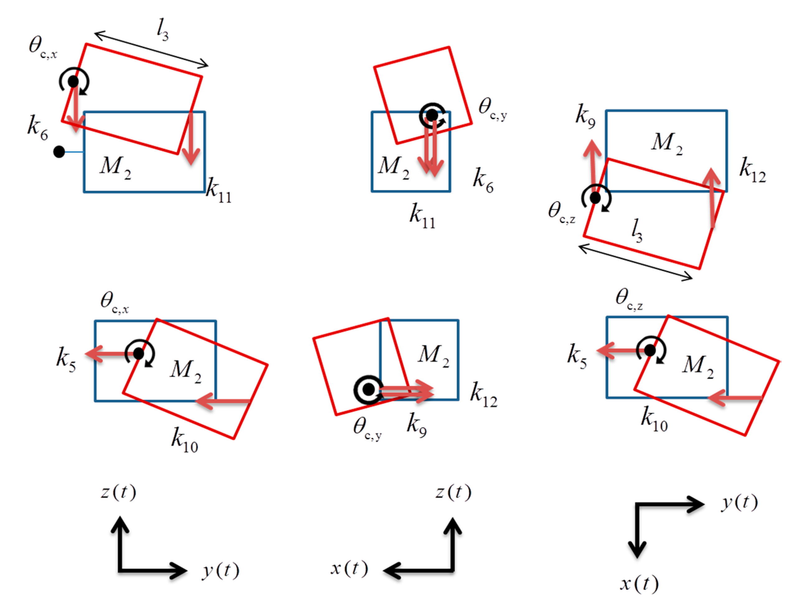
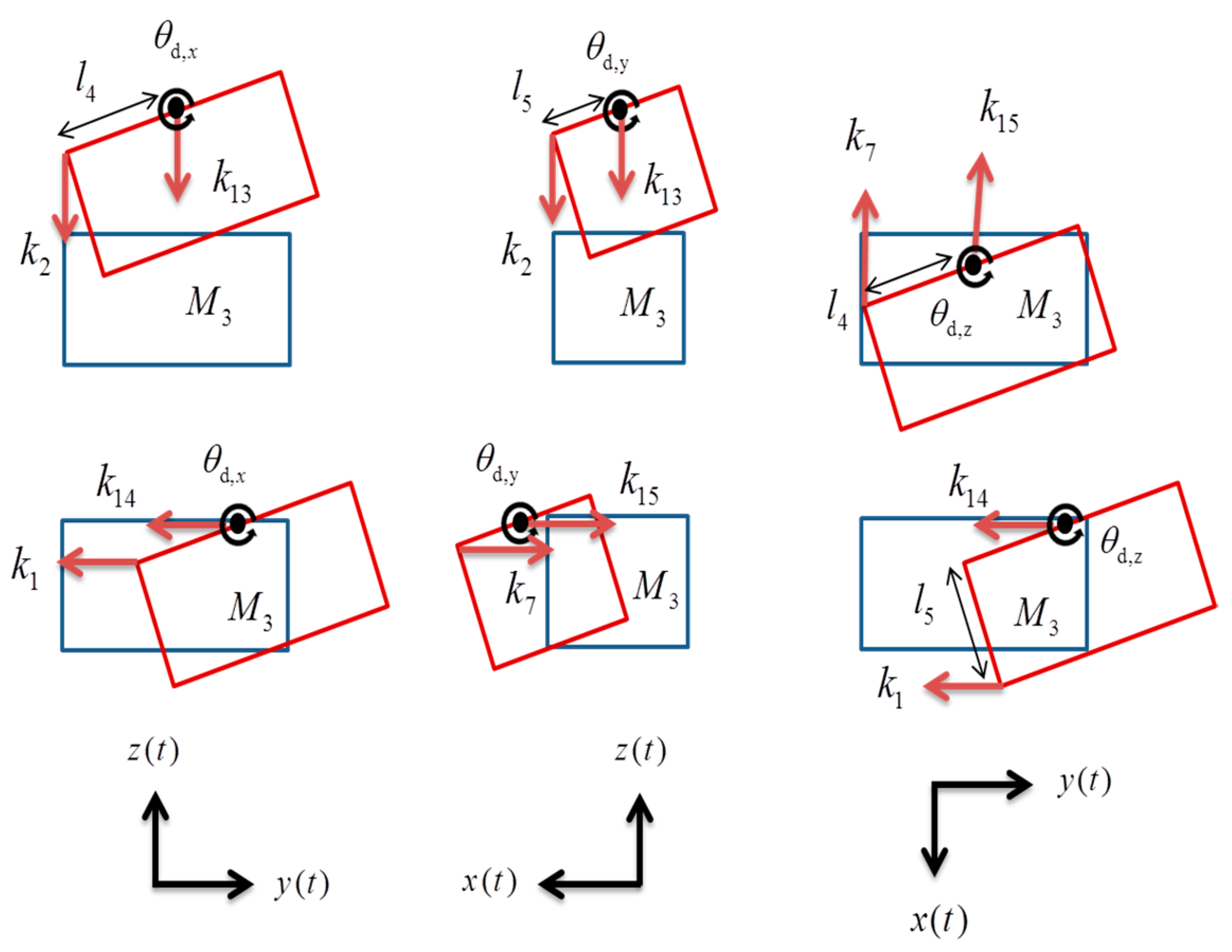
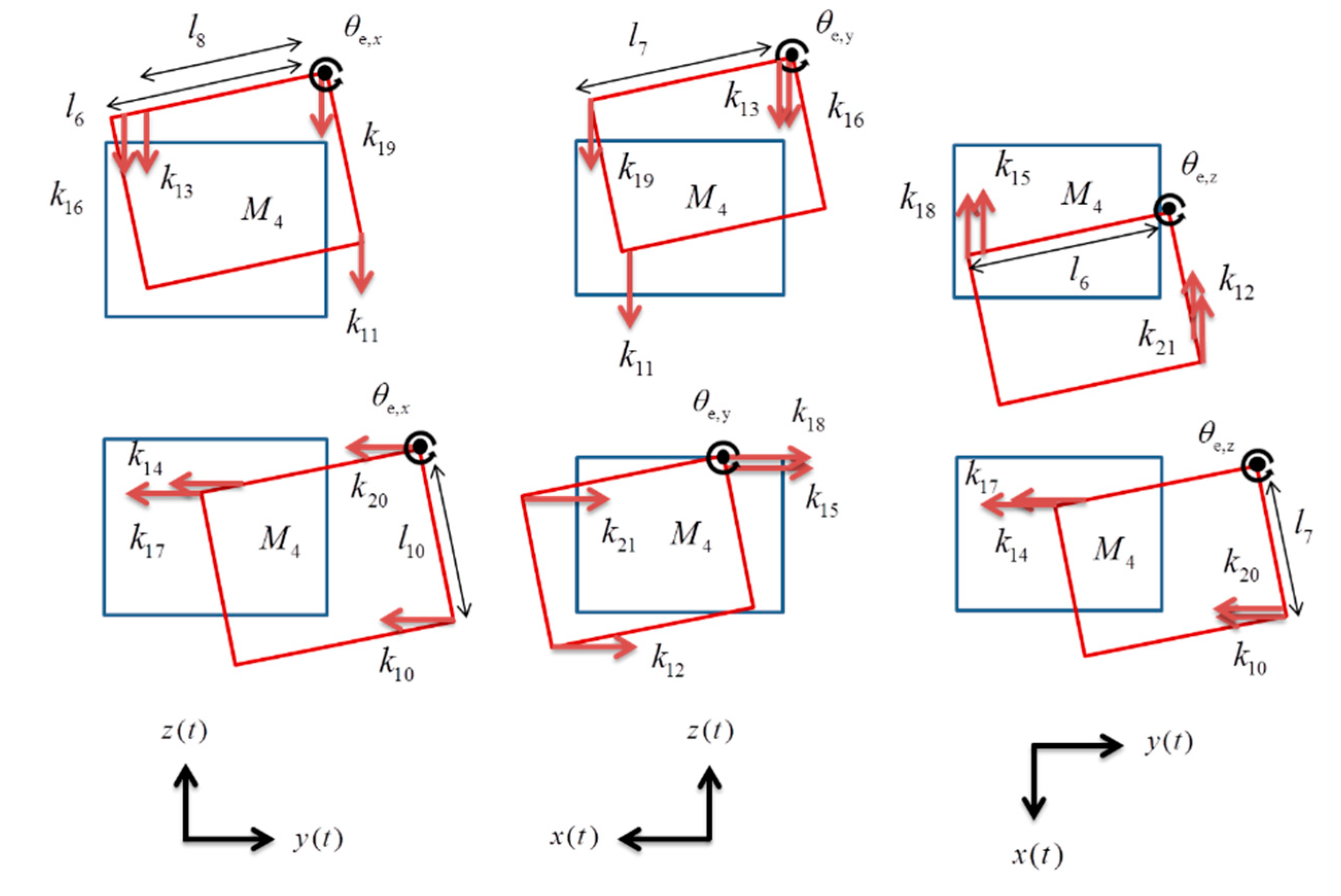
3.1. Mathematical Modeling and Derivation of Equations

Mathematical modeling is the foremost step, which requires drawing the free-body diagrams of the masses under study. A free-body diagram is a graphical illustration used to visualize the magnitude and direction of all forces acting on an object, and the resulting reactions in a given situation [20]. It is a 2D figure often in the form of a box with the forces shown as straight arrows and moments as round arrows, with arrowheads showing the directions. Each mass should be illustrated in three planes separately. The headlamp assembly comprises four components; hence, there will be 12 free-body diagrams showing the forces and moments.

The second step is modeling the motion of a dynamic system in terms of the equations of motion. The number of equations that can completely define the system must be equal to the total number of DOFs considered. This paper proposes a 23 DOF system; therefore, 23 equations are derived using Newton’s second law of motion. A standard equation of motion for a single DOF system is shown below.

$$m\ddot{x}+c\dot{x}+kx=F\left(t\right)$$

(1)

As no damping element is considered in this study, the term containing the damping coefficient will be excluded. The term $F_T$ is defined as the applied excitation to the system. In the present case, the excitation force was applied to the outer housing because external forces were applied by the automobile chassis to the headlamp module through the housing.

In Figure 2, $M_1$ is shown in terms of the free-body diagrams in three planes. Each set of diagrams shows the direction of linear displacements and their reactions. The restoring forces or reactions of the linear displacements are shown by the arrows in red, with the arrowheads pointing toward the direction of the forces. These can also be referred to as the restoring forces of stiffness elements. The components before and after the displacement are highlighted in blue and red boxes, respectively.

There are a large number of stiffness elements in the model; hence, each k value is numbered for reference. The applied angular displacements are also shown as round arrows in black, about the points of rotation of each component. The direction of rotation is both clockwise and counter-clockwise, depending on the conditions. The letters in subscripts of the terms like ${\theta }_{b,x}$ provide information on the axis and point of rotation. For example, in ${\theta }_{b,x}$, the rotation is about the x-axis and occurs at point b. The corresponding equations of motion for the projection unit are as follows:

$$M_1{\ddot{z}}_1+k_2\left(z_1-z_3-l_1{\theta }_{b,x}\right)+k_3{z}_1+k_6\left(z_1-z_2+l_2{\theta }_{b,x}\right)=0$$

(2)

$$M_1{\ddot{y}}_1+k_1\left(y_1-y_3+l_1{\theta }_{b,x}\right)+k_4{y}_1+k_5\left(y_1-y_2+l_2{\theta }_{b,x}\right)=0$$

(3)

$$M_1{\ddot{x}}_1+k_7\left(x_1-x_3\right)+k_8{x}_1+k_9\left(x_1-x_2-l_2{\theta }_{b,y}\right)=0$$

(4)

The set of governing equations for angular motion are as follows:

$$J_1{\ddot{\theta }}_{b,x}+k_2\left(z_1-z_3-l_1{\theta }_{b,x}\right)l_1-k_5\left(y_1-y_2+l_2{\theta }_{b,x}\right)l_2=0$$

(5)

$$J_1{\ddot{\theta }}_{b,y}+k_9\left(x_1-x_2-l_2{\theta }_{b,y}\right)l_2=0$$

(6)

$$J_1{\ddot{\theta }}_{b,z}+k_7\left(x_1-x_3+l_1{\theta }_{b,z}\right)l_1=0$$

(7)

In this study, the effect of rotation on each stiffness element was considered, thereby including terms like $l_2{\theta }_{b,x}$ in the equations. Here, the arc length is measured when a body rotates at an angle $\theta$. If the angle of rotation is very small, then the arc is considered as a straight line. At the locations where the contact support is mutual between two components, relative displacement is assumed. In Figure 3,$M_2$ is shown in terms of the free-body diagrams in three planes.

Based on the figures above, the equations of motion of the aiming unit are expressed as follows:

$$M_2{\ddot{z}}_2+k_6\left(z_2-z_1\right)+k_{11}\left(z_2-z_4-l_3{\theta }_{c,x}\right)=0$$

(8)

$$M_2{\ddot{y}}_2+k_5\left(y_2-y_1\right)+k_{10}\left(y_2-y_4\right)=0$$

(9)

$$M_2{\ddot{x}}_2+k_9\left(x_2-x_1\right)+k_{12}\left(x_2-x_4\right)=0$$

(10)

$$J_2{\ddot{\theta }}_{c,x}+k_{11}\left(z_2-z_4-l_3{\theta }_{c,x}\right)l_3+k_{10}\left(y_2-y_4\right)l_3=0$$

(11)

$$J_3{\ddot{\theta }}_{c,z}-k_{12}\left(x_2-x_4+l_3{\theta }_{c,z}\right)l_3=0$$

(12)

$$J_2{\ddot{\theta }}_{c,y}=0$$

(13)

Similarly, the free-body diagrams of the bracket unit are shown below in Figure 4.

The equations of motion for bracket unit $M_3$ are as follows:

$$M_3{\ddot{z}}_3+k_2\left(z_3-z_1-l_4{\theta }_{d,x}\right)+k_{13}\left(z_3-z_4\right)=0$$

(14)

$$M_3{\ddot{y}}_3+k_1\left(y_3-y_1+l_4{\theta }_{d,x}\right)+k_{14}\left(y_3-y_4\right)=0$$

(15)

$$M_3{\ddot{x}}_3+k_{15}\left(x_3-x_4\right)+k_7\left(x_3-x_1-l_5{\theta }_{d,y}\right)=0$$

(16)

The equations for angular displacement are expressed as:

$$J_3{\ddot{\theta }}_{d,x}+k_2\left(z_3-z_1-l_4{\theta }_{d,x}\right)l_4=0$$

(17)

$$J_3{\ddot{\theta }}_{d,z}-k_7\left(x_3-x_1+l_4{\theta }_{d,z}\right)l_4-k_1\left(y_3-y_1+l_5{\theta }_{d,z}\right)l_5=0$$

(18)

$$J_3{\ddot{\theta }}_{d,y}+k_2\left(z_3-z_1-l_4{\theta }_{d,y}\right)l_4+k_7\left(x_3-x_1-l_5{\theta }_{d,y}\right)l_5=0$$

(19)

Figure 5 shows the forces acting on the housing. Because this part is connected to the automobile chassis, it is under the influence of random forces.

In the proposed method, forcing conditions were applied to the housing in the vertical (z-axis) direction. The governing equations for $M_4$ are as follows:

$$M_4{\ddot{z}}_4+k_{19}{z}_4+k_{11}\left(z_4-z_3+l_{10}{\theta }_{e,x}\right)+k_{16}\left(z_4-l_6{\theta }_{e,x}\right)+k_{13}\left(z_4-z_1-l_8{\theta }_{e,x}\right)=F$$

(20)

$$M_4{\ddot{y}}_4+k_{17}\left(y_4+l_6{\theta }_{e,x}\right)+k_{14}\left(y_4-y_1+l_6{\theta }_{e,x}\right)+k_{20}{y}_4+k_{10}\left(y_4-y_3+l_{10}{\theta }_{e,x}\right)=0$$

(21)

$$M_4{\ddot{x}}_4+k_{21}\left(x_4+l_7{\theta }_{e,y}\right)+k_{18}{x}_4+k_{15}\left(x_4-x_1\right)+k_{12}\left(x_4-x_3+l_{10}{\theta }_{e,y}\right)=0$$

(22)

This is the largest part of the headlamp assembly, and each component is connected to it. It is attached to the chassis through fixed connections at multiple points. In the developed model, two supports were selected for analysis. In addition, there is an origin of rotation at the middle corner, expressed as point e in Figure 1. The equations for rotation are expressed as follows:

$$J_4{\ddot{\theta }}_{e,y}+k_{19}\left(z_4-l_7{\theta }_{e,y}\right)l_7+k_{11}\left(z_4-z_3-l_7{\theta }_{e,y}\right)l_7-k_{12}\left(x_4-x_3+l_{10}{\theta }_{e,y}\right)l_{10}=0$$

(23)

$$J_4{\ddot{\theta }}_{e,x}+k_{16}\left(z_4-l_6{\theta }_{e,x}\right)l_6+k_{13}\left(z_4-z_1-l_8{\theta }_{e,x}\right)l_8-k_{10}\left(y_4-y_3+l_{10}{\theta }_{e,x}\right)l_{10}=0$$

(24)

$$\begin{gathered} J_4{\ddot{\theta }}_{e,z}-k_{18}\left(x_4+l_6{\theta }_{e,z}\right)l_6-k_{15}\left(x_4-x_1+l_8{\theta }_{e,z}\right)l_8 \\ -k_{20}\left(y_4+l_7{\theta }_{e,z}\right)l_7-k_{10}\left(y_4-y_3+l_7{\theta }_{e,z}\right)l_7=0 \end{gathered}$$

(25)

3.1.1. Forcing Conditions

The proposed method aims to predict the force transmitted through the headlamp assembly. The assembly must be excited by external forces at one end to obtain the value of the force transmitted to the other end. In actual driving conditions, the vehicle moves across several even and uneven road surfaces. A series of random excitation forces is applied to the headlamp every second; thus, it is challenging to find a trend in the values. To reproduce the actual driving conditions in the simulation, an experiment was conducted using an accelerometer mounted on the dashboard of a vehicle. The accelerometer could not be mounted at the back side because the readings were to be obtained for the headlamps. There was a possibility to mount it right above the headlamp but it could not be fixed there properly. While driving through the non-uniform surfaces, it may get loose and record false readings. It should be as much near to the center of the vehicle as possible, so that the pitch of vehicle has minimum effect on the vertical acceleration readings. Other factors that could influence the accelerometer sensitivity are temperature and mount type. A DC-response accelerometer was used because it can perform well in shock applications where we need to integrate the acceleration data. Other types will have an intrinsic decay function that can result in significant error. An accelerometer with sensitivity of 10 mV/g and frequency range of 1 to 10,000 Hz (−5%) was used in this experiment. The vehicle was driven through even and uneven roads, and two sets of time-acceleration data were collected in each case (case I and case II). The following directions were assumed: vertical to the road surface (z-axis), direction of vehicle travel (x-axis), and direction transverse to vehicle travel (y-axis). The data were collected in seconds, and the duration of the experiment varied for each case. Figure 6 illustrates the road surface conditions for the even and uneven cases.

The data obtained for case I is shown in Figure 7. Figure 7a plots the magnitude of acceleration with respect to time, with values ranging between 9.9 and 10.2 $\mathrm{m}/{\mathrm{s}}^2$. The total mass of the four components under study is approximately 3 kg. The product of the total mass and acceleration provides the magnitude of the force applied. The obtained magnitude of force in case I reached 31 N, with the experiment lasting for 300 s and the vehicle driven along an even road at constant speed; the plot of the data is shown in Figure 7b.

The data for case II is shown below in Figure 8. In case II, the acceleration reached a maximum of 20.72 $\mathrm{m}/{\mathrm{s}}^2$. The vehicle was driven across bumps and potholes, which led to this abrupt increase in magnitude. Figure 8b shows the force applied in case II. The maximum amplitude of the force is approximately 63 N, which is double than that in case I. The data for case II is shown below.

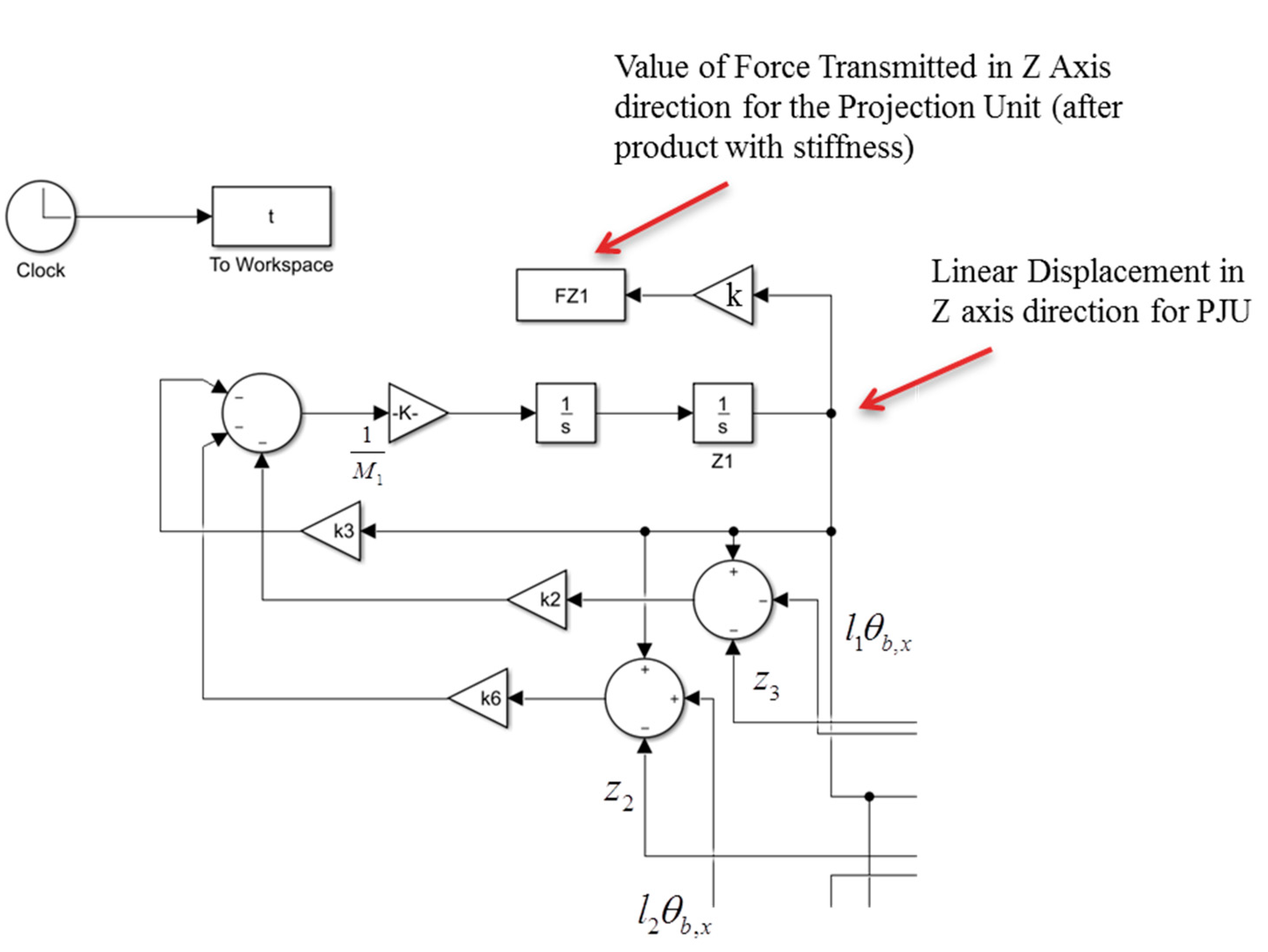
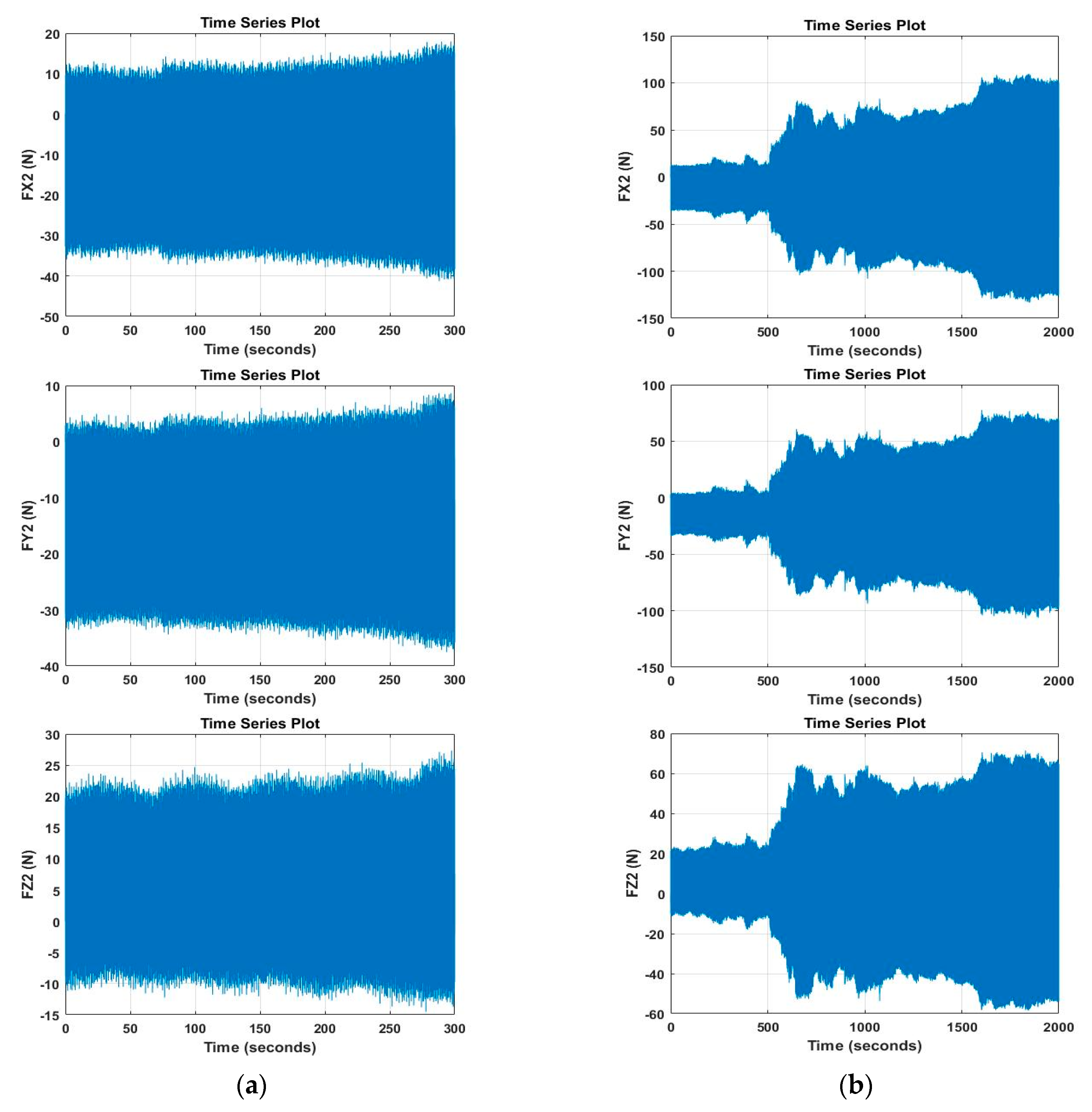
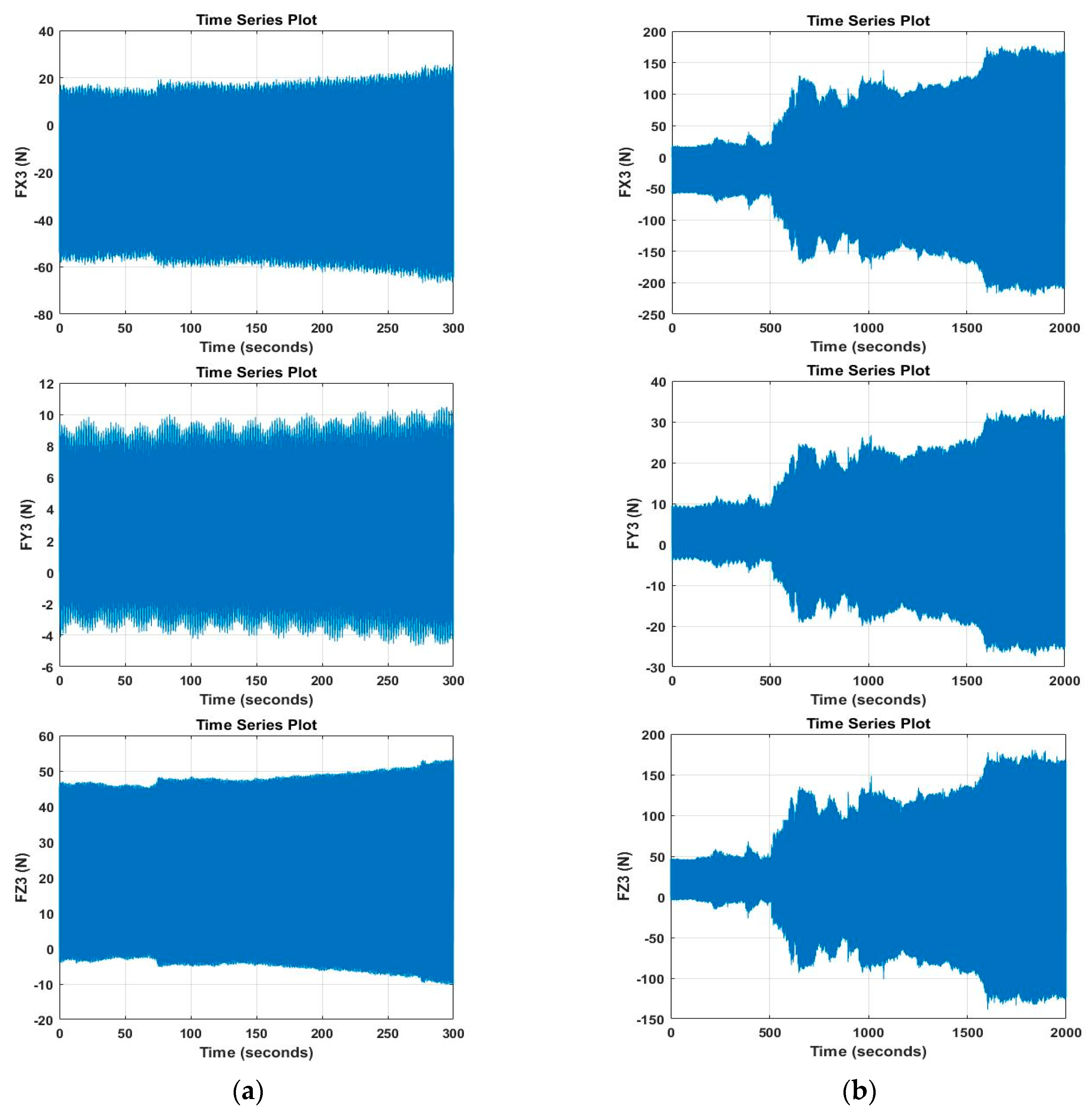
3.1.2. Force Transmission

The amount of force transferred from the automobile chassis to the headlamp module is measured in terms of force transmission. The standard equation for force transmitted is [21].

$$F_T=c\left(\dot{x}-\dot{y}\right)+k\left(x-y\right)=-m\ddot{x}$$

(26)

Damping was not considered, and the term $k\left(x-y\right)$ was calculated using MATLAB GUI. In Figure 3, the displacement of the housing along the z-axis was multiplied by the stiffness to obtain the magnitude of the force transmitted. Similarly, $F_T$ was obtained by 12 linear displacement values of the components in three dimensions.

3.2. Solution of Equations

Vibration analysis was conducted to determine the mass displacements in the system. This provides an understanding of how the internal components are affected by the external forcing conditions. To obtain the linear or angular displacement values from the above equations, MATLAB was utilized. First, the equations were rearranged in the following form (Equation (2) has been changed to the following form, for example.)

$${\ddot{z}}_1=\frac{-k_2\left(z_1-z_3-l_1{\theta }_{b,x}\right)-k_3{z}_1-k_6\left(z_1-z_2+l_2{\theta }_{b,x}\right)}{M_1}$$

(27)

After the double integration of the above equation, linear displacement of the projection unit along the z-axis can be obtained. The Simulink model for this equation is shown below in Figure 9.

All the terms were added and divided by the mass, and then two integration blocks were used to obtain the displacement. For the other equations, models were developed and solved to determine the response of the system. Because the system is coupled, the output of one equation affects other linked equations. A small change in variables, such as mass or stiffness, at one point can alter the solution of some other blocks.

In the case of angular displacement, mass $M$ was replaced by the angular moment of inertia $J$ and linear displacement by $\theta$. The equation used to develop Simulink model for the rotation is expressed as follows (Equation (25) has been changed to the following form, for example.).

$${\ddot{\theta }}_{e,z}=\frac{+k_{18}\left(x_4+l_6{\theta }_{e,z}\right)l_6+k_{15}\left(x_4-x_3+l_8{\theta }_{e,z}\right)l_8+k_{20}\left(y_4+l_7{\theta }_{e,z}\right)l_7+k_{10}\left(y_4-y_2+l_7{\theta }_{e,z}\right)l_7}{J_4}$$

(28)

After the equation is integrated twice, the value of the angle of rotation is obtained for the housing at point e, about the z-axis. All the equations of rotation were simulated the same way as above, and angles of rotation were obtained.

Developing the GUI

A GUI is an application of MATLAB used to develop a user-friendly solution environment. It is very convenient for solving a system when the input variables need to be varied for analysis. For the headlamp assembly, the developed Simulink model was linked with the GUIDE (Graphical User Interface Development) application to create the GUI. Force transmission plots were added in the “.fig” file. Several variables, such as mass, length, stiffness, and moment of inertia were also added (see Table 1). Stiffness magnitudes values used in the GUI ranged from 15,000–18,000 $N/m$. These can be varied and any required value can be used to run the solution. Angular moments of inertia were calculated by assuming each body as a sphere. A time function is included in the GUI, which can be utilized to alter the solution time of the model. When the “Simulate & Plot” button (Figure 10) is pressed, Simulink runs the solution and plots the results on the GUI. All variables shown on the interface can be varied with just one click, and system can be solved again. The developed GUI is demonstrated below.

4. GUI Results

Since there are two cases of forcing conditions applied, there are also two sets of solutions from the equations of motion. First, the acceleration data from the even road surface (case I) was applied to the Simulink model and solved. Stiffness values at different locations were chosen randomly. For a fixed support, higher stiffness values are often considered; therefore, stiffness magnitudes are in the thousands. However, it can be any number above or below those used in the GUI. Then, the acceleration data obtained from uneven road surface (case II) was applied and simulated. The results from the GUI were compared for each of the components under both excitation conditions.

Projection Unit

Figure 11 compares the values of force in $M_1$ in both cases. The plots on the left and right side are for case I and case II, respectively. It is clear from the figure that the projection unit encountered greater force in case II because of the higher peaks of vertical acceleration. The simulation was conducted for the whole input force data for up to 300 s and 2000 s for case I and case II, respectively. A significant amount of time was required to completely solve the system.

Based on the above results, the magnitudes of force are approximately 29.12 N, 6.69 N, and 23.48 N for the x-, y-, and z-axis in case I, and 94 N, 9 N, and 65 N in case II, respectively. For the projection unit, the force transmission in case II is very high, approximately three times greater along the x- and z-axis. However, the variation in amplitude is minimal along the y-axis.

The GUI results for $M_2$ are shown below in Figure 12. This figure compares the force transmitted through the aiming unit in both cases. A significant increase can be observed in the values for case II. The magnitudes of force along the x-, y-, and z-axis were 41 N, 37 N, and 27 N in case I, and 132 N, 107 N, and 71 N in case II, respectively. There was a considerable increase in force amplitudes in all the axes compared with the projection unit. One reason could be the effect of rotation of $M_1$ on the aiming unit. Because the aiming unit also has its own origin of rotation at point c, this relative rotation between two masses increased the displacements in $M_2$, and hence the values of $F_T$.

Figure 13 shows the plots comparing $F_T$ magnitudes in the bracket unit. The amplitude of $M_3$ increased by more than three times in case II when compared with case I. The values were 67 N, 10 N, and 53 N in the direction of the x-, y-, and z-axis, respectively, and the values were 222 N, 33 N and 181 N in case II, respectively.

The force transmitted through the outer housing is shown in Figure 14. It gained the amplitude of 46 N, 39 N, and 49 N in the x-, y-, and z-direction, respectively. The magnitude was lower compared with the bracket unit. Because the bracket unit has lower mass, higher displacement values were obtained by Simulink; hence, additional force was transmitted compared with the housing, aiming unit, or projection unit.

The above results show a significant increase in the force transmitted in case II, except for the projection unit in the y-axis direction. The maximum force was transmitted through the bracket unit in the x-axis direction. The minimum amount of force was gained by the projection unit in the y-direction. These results are summarized in

Table 2. Comparison of force transmission results from GUI for case I and case II.

Component	Force Transmitted (±5)	Case I	Case II	Increase
Projection Unit $M_1$	FX1	−29	−94	65 (224%)
	FY1	6	9	3 (150%)
	FZ1	23	65	42 (282%)
Aiming Unit $M_2$	FX2	−41	−132	91 (321%)
	FY2	−37	−107	70 (289%)
	FZ2	27	71	44 (262%)
Bracket Unit $M_3$	FX3	−67	−222	155 (331%)
	FY3	10	33	23 (330%)
	FZ3	53	181	128 (341%)
Housing $M_4$	FX4	−47	−155	108 (329%)
	FY4	−39	−127	88 (325%)
	FZ4	49	150	101 (306%)

.

5. Conclusions and Future Plans

In this study, a multi-DOF modeling procedure for an automotive LED headlamp assembly was proposed. This technique was utilized to predict the force transmitted through the headlamp under severe conditions when a vehicle moves across uneven road surfaces. The major contributions of this paper are as follows:

1.

A new concept for the multi-DOF modeling of an automotive LED headlamp assembly was introduced. This type of study on vibration and dynamics has not been performed on an LED headlamp; thus, a vibration model for the headlamp module was proposed to simulate the system under the desired boundary conditions. Using LEDs in automotive lighting is an emerging concept that requires additional validation and standardization studies;

2.

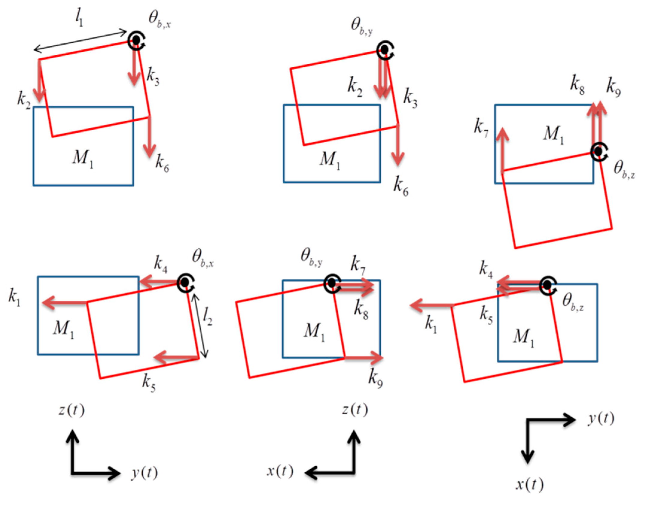
The proposed methodology provides an understanding of the dynamics of each component of the system. In the present work, an effort has been made to determine the dynamics of the LED headlamp module to determine whether the system can withstand the forcing conditions applied by the vehicle moving across an uneven road to ensure the reliability of the equipment. Linear and angular displacements of the components of the headlamp were determined using Newton’s second law, and then the force transmitted through each body was calculated using MATLAB;

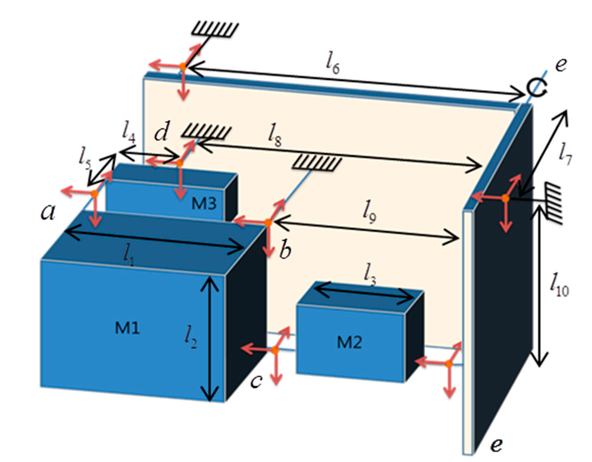
3.

A 3D model of the system was developed. Each mass component was considered as a cube with realistic parameters, the same as the actual device. There were four main components considered in the system: projection unit, aiming unit, bracket unit, and outer housing. The motion of each component was considered in three dimensions including a rotation point for each. A vibration model with 23 DOFs was developed, and a system of equations of motion was obtained. These equations were solved in Simulink, and the linear and angular displacements were calculated using a GUI application in MATLAB;

4.

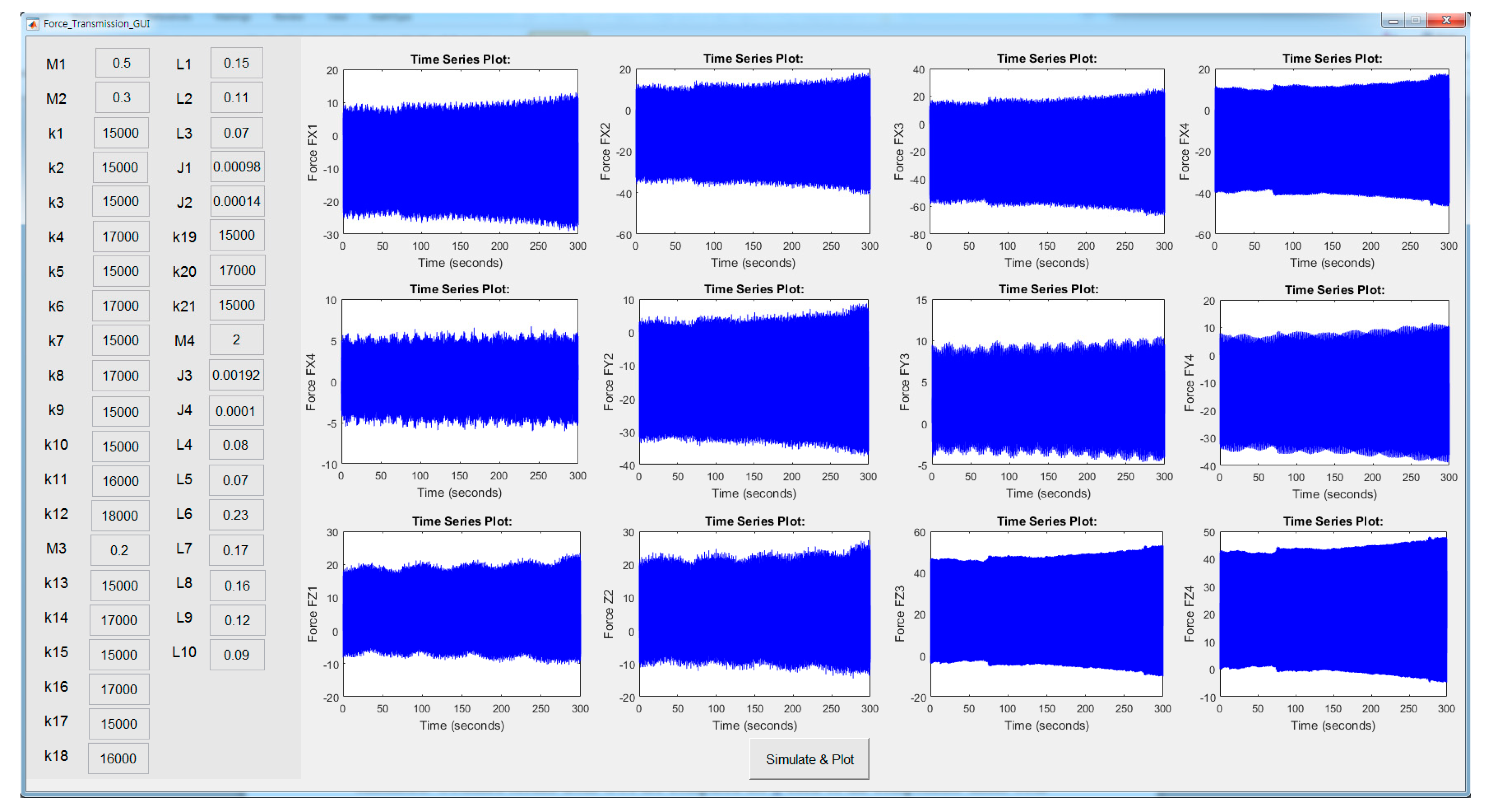
The GUI was developed to simulate the system under several conditions. The GUI provides a user-friendly interface that can be used to solve the model with just one click. Even a basic knowledge of MATLAB is sufficient to obtain results. Simulink was linked with the GUIDE application of MATLAB to obtain a UI environment. Parameters such as stiffness, length, and mass were included in this application, which can be altered to observe the behavior of the system;

5.

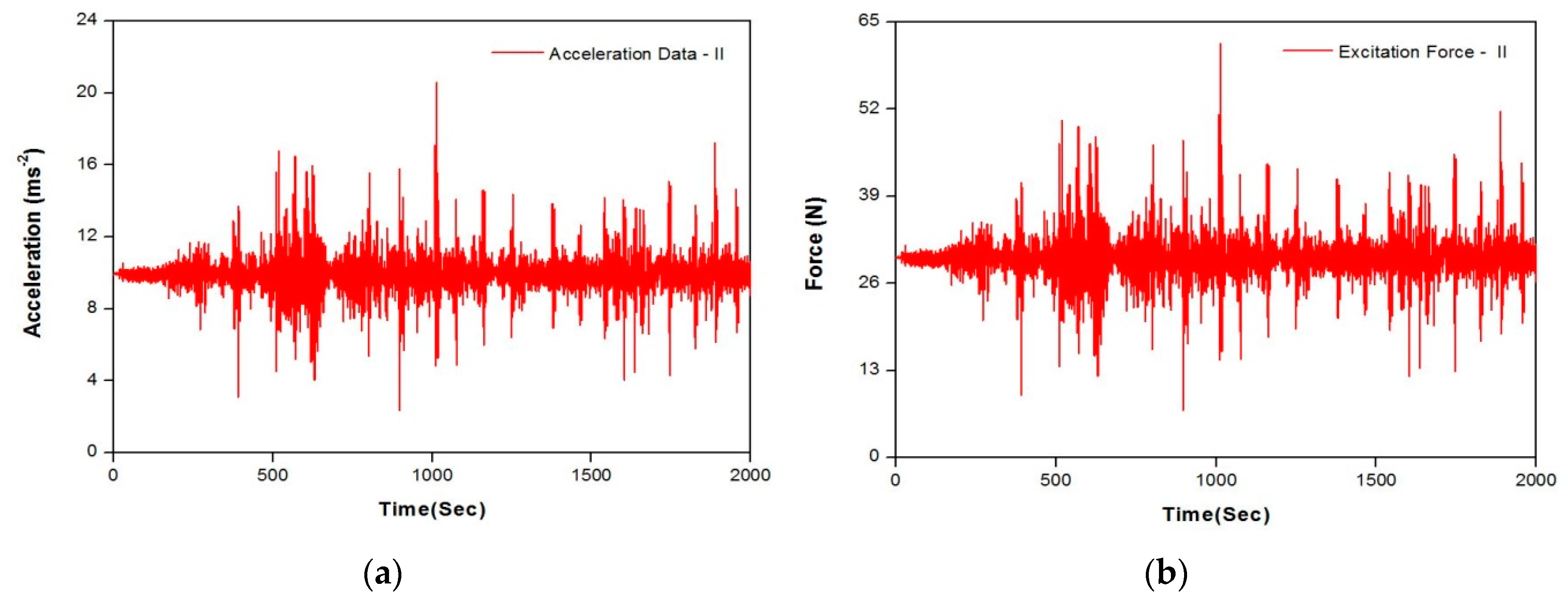
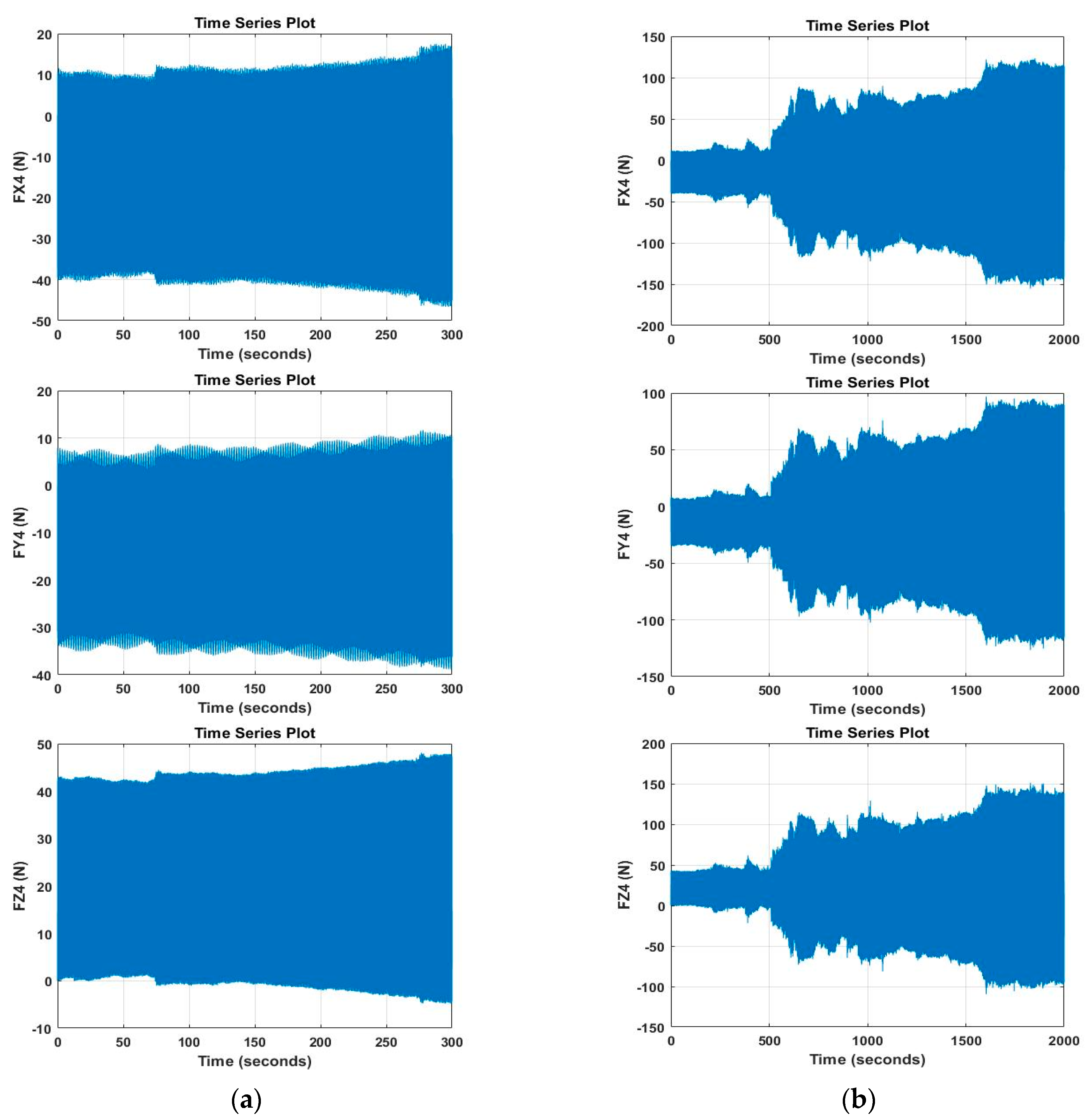
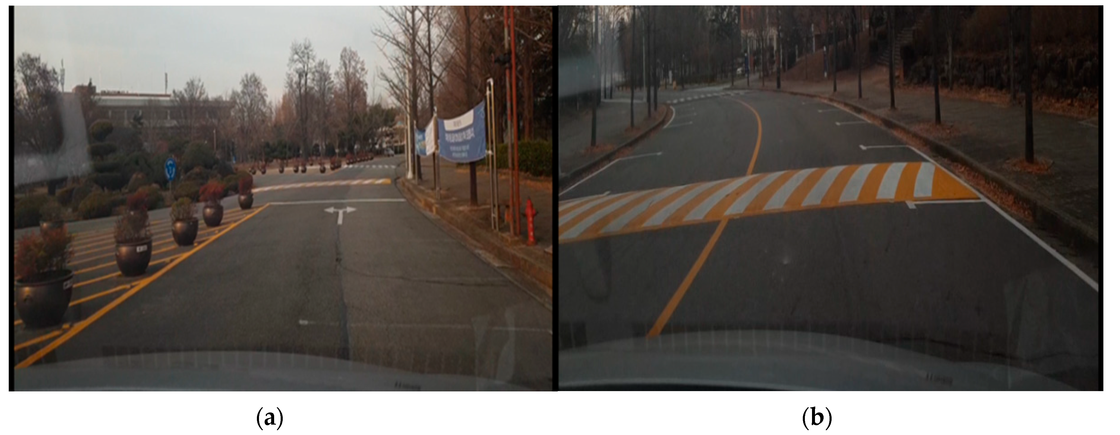
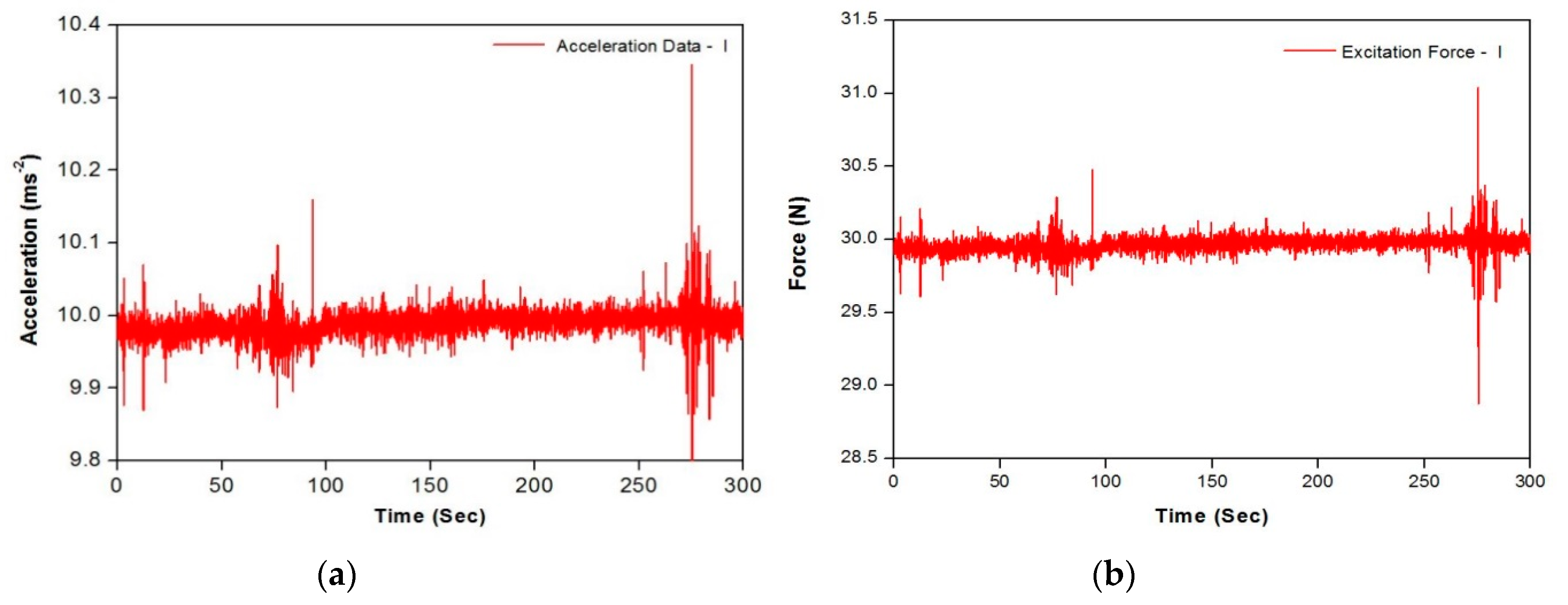
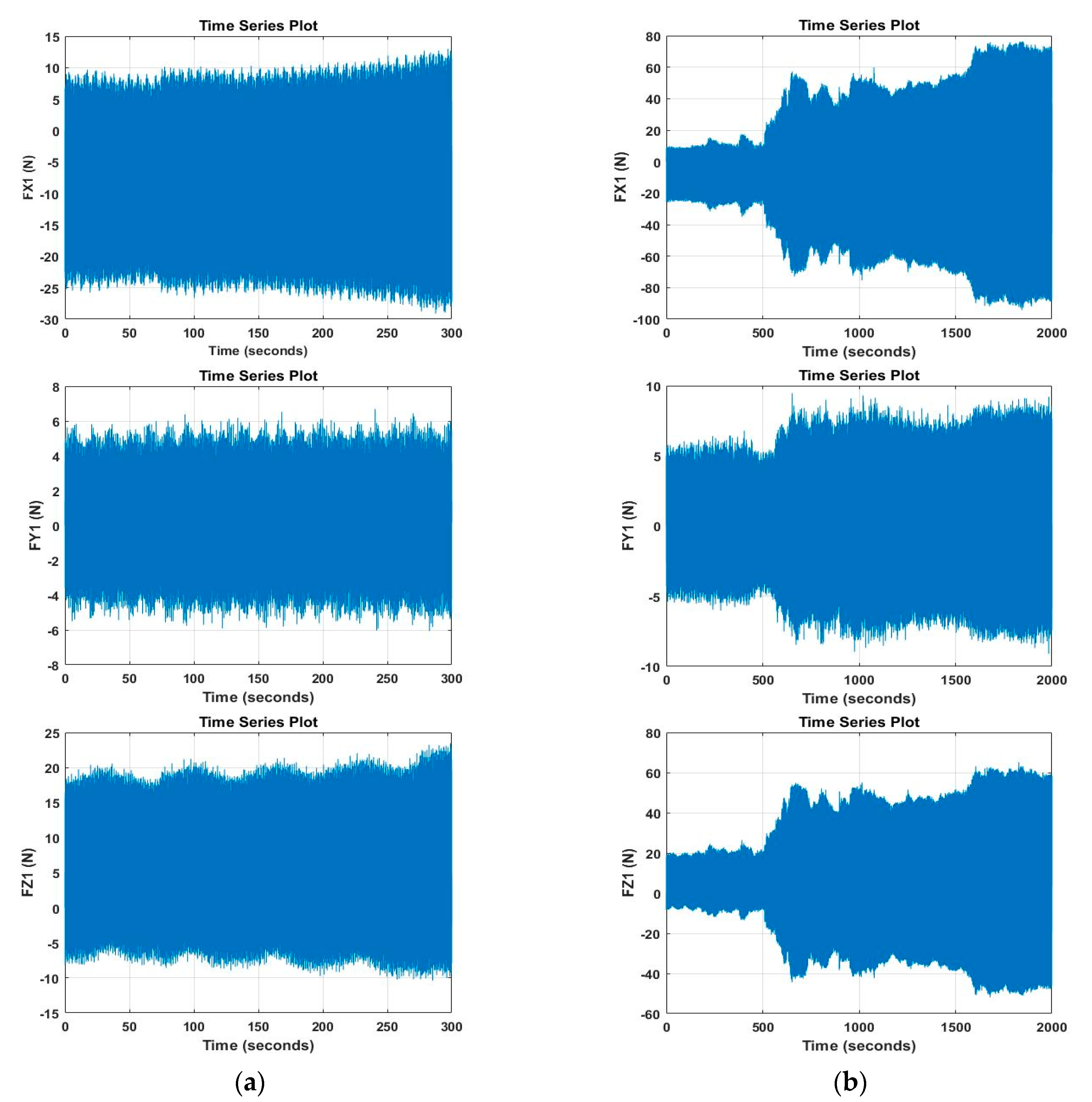
An experiment was conducted to apply the forcing conditions that actually occur in an automobile chassis. The acceleration data in each axis was obtained using an accelerometer mounted on the vehicle. Applying this data to the developed model provided the fluctuations of the system that occur on the road. Then, the forces transmitted from the automobile chassis to the headlamp components were compared for the two cases of automobile movement. In addition, using the real data from road provided approximately the real road conditions to the simulation; hence, extensive experimental work could be avoided, and authentic anticipation of results can be achieved

This analysis successfully identified the locations in the system with higher displacements and forces. The results can be used for dynamic analysis of automotive lighting systems equipped with sensitive LEDs, and to identify the components that are most affected in uneven road conditions to help manufacturers in dynamic stiffness optimization. In the past, FRF, frequency response functions were calculated and compared for different assemblies. This technique has a drawback because gaps between components were considered. In contrast, this paper has successfully obtained beneficial outcomes by considering stiffness supports between headlamp assembly components.

This article has developed a new model using. The projection unit is the main component that can be assembled with more stiff supports than the housing to prevent damage and improve the reliability of the system. In particular, it can be used for the analysis of the bolt-loosening phenomenon and the design of an automotive LED headlamp-aiming mechanism focused on vibration and durability. Future work includes the optimization of the proposed model by including more components of the headlamp assembly, such as electronic controllers and thermal management equipment to develop a complete setup for simulating the whole assembly simultaneously.

References

1. Dewar, R.; Olson, P. Human Factors in Traffic Safety, 2nd ed.; Lawyers & Judges Publishing Company: Tucson, AZ, USA, 2007. [Google Scholar]
2. Bullough, J.; Donnell, E.; Rea, M.S. To illuminate or not to illuminate: Roadway lighting as it affects traffic safety at intersections. Accid. Anal. Prev. 2013, 53, 65–77. [Google Scholar] [CrossRef] [PubMed]
3. Kim, D. Study of Optimized Tuning in Full AFLS Head Lamps. Lect. Notes Electr. Eng. 2012, 196, 1719–1731. [Google Scholar]
4. Moiseev, M.A.; Doskolovich, L.L.; Kazanskiy, N.L. Design of high-efficient freeform LED lens for illumination of elongated rectangular regions. Opt. Express 2011, 19, A225–A233. [Google Scholar] [CrossRef] [PubMed]
5. Aslanov, E.R.; Doskolovich, L.L.; Moiseev, M.A.; Bezus, E.A.; Kazanskiy, N.L. Design of an optical element forming an axial line segment for efficient LED lighting systems. Opt. Express 2013, 21, 28651–28656. [Google Scholar] [CrossRef]
6. Kazanskiy, N.L.; Skidanov, R. Binary beam splitter. Appl. Opt. 2012, 51, 2672. [Google Scholar] [CrossRef]
7. Doskolovich, L.L.; Dmitriev, A.Y.; Moiseev, M.A.; Kazanskiy, N.L. Analytical design of refractive optical elements generating one-parameter intensity distributions. J. Opt. Soc. Am. A 2014, 31, 2538–2544. [Google Scholar] [CrossRef] [PubMed]
8. Abulkhanov, S.R.; Gorjainov, D.S.; Skuratov, D.L. Optimization of strength characteristics of aircraft lighting devices by building their virtual models. Bull. Samara State Aerosp. Univ. 2012, 5, 72–78. [Google Scholar]
9. Kharche, S.; Karajagi, P.; Kulkarni, R.; Siddhant College of Engineering. Design Development and Vibration Analysis of MCM300 Headlamp. Int. J. Eng. Trends Technol. 2016, 38, 168–175. [Google Scholar] [CrossRef]
10. Dascotte, E. Applications of Finite Element Modal Updating Using Experimental Modal Data. Sound Vib. 1991, 25, 22–26. [Google Scholar]
11. Performance requirements for motor vehicle headlamps, SAE J1383 Apr 8. Available online: https://law.resource.org/pub/us/cfr/ibr/005/sae.j1383.1985.html (accessed on 21 August 2020).
12. United Nations Economic Commission for Europe, Regulations 101–120. Available online: https://www.unece.org/?id=39146 (accessed on 21 August 2020).
13. United Nations Economic Commission for Europe, Regulations 121–140. Available online: https://www.unece.org/?id=39147 (accessed on 21 August 2020).
14. Schrader, C.D.; Hilburger, F.K.N. Development and Correlation of Three Axes Random Vibration Simulation on Automotive Lighting. SAE Tech. Paper Ser. 2005 2005, 2005–01–1570. [Google Scholar] [CrossRef]
15. Zhang, Y.; Usman, M. Life Prediction for Lighting Bulb Shield Designs Subjected to Random Vibration. SAE Tech. Paper Ser. 1999 1999, 1999–01–0705. [Google Scholar] [CrossRef]
16. Roucoules, C.; Chemin, F.; Cros, C. FRF Prediction and Durability of Optical Module and Headlamp. Valeo Lighting Syst. 2010, 4373–4382. [Google Scholar]
17. Kim, B.; Hong, D.; Park, J. Estimation of transmitted force through aiming bolt in headlamp module using lumped parameter modeling. Vibroengineering PROCEDIA 2020, 30, 15–19. [Google Scholar] [CrossRef]
18. Etienne, B.; Jean, P.B. Prise En Compte De non linearite de Frottement Dans Les Optiques De Phare, SDTOOLS, Internal Reports.
19. Rao, S.S. Mechanical Vibrations, 5th ed.; Addison Wesley: Boston, MA, USA, 1995. [Google Scholar]
20. Puri, A. The art of free-body diagrams. Phys. Educ. 1996, 31, 155–157. [Google Scholar] [CrossRef]
21. Steidel, R.F. An Introduction to Mechanical Vibrations, 3rd ed.; John Wiley & Sons, Inc: New York, NY, USA, 1989. [Google Scholar]
Figure 1. Demonstration of four components.
Applsci 10 05906 g001
Figure 2. Free-body diagrams of the main projection unit.
Applsci 10 05906 g002
Figure 3. Free-body diagrams of the aiming unit.
Applsci 10 05906 g003
Figure 4. Free-body diagrams of the bracket unit.
Applsci 10 05906 g004
Figure 5. Free-body diagrams of the housing.
Applsci 10 05906 g005
Figure 6. Images from video recording of data collection experiments: (a) case I; (b) case II.
Applsci 10 05906 g006
Figure 7. Input data for case I: (a) acceleration data; (b) excitation force.
Applsci 10 05906 g007
Figure 8. Input data for case II: (a) acceleration data; (b) excitation force.
Applsci 10 05906 g008
Figure 9. Simulink model for force transmission.
Applsci 10 05906 g009
Figure 10. Demonstration of the developed graphical user interface (GUI).
Applsci 10 05906 g010
Figure 11. Force transmission results for projection unit from GUI: (a) results for case I; (b) results for case II.
Applsci 10 05906 g011
Figure 12. Force transmission results for aiming unit from GUI: (a) results for case I; (b) results for case II.
Applsci 10 05906 g012
Figure 13. Force transmission results for bracket unit from GUI: (a) results for case I; (b) results for case II.
Applsci 10 05906 g013
Figure 14. Force transmission results for bracket unit from GUI. (a) Results for case I; (b) Results for case II.
Applsci 10 05906 g014