Modeling and NVH Analysis of a Full Engine Dynamic Model with Valve Train System


Abstract
1. Introduction
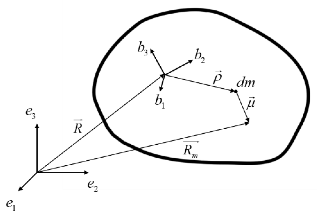
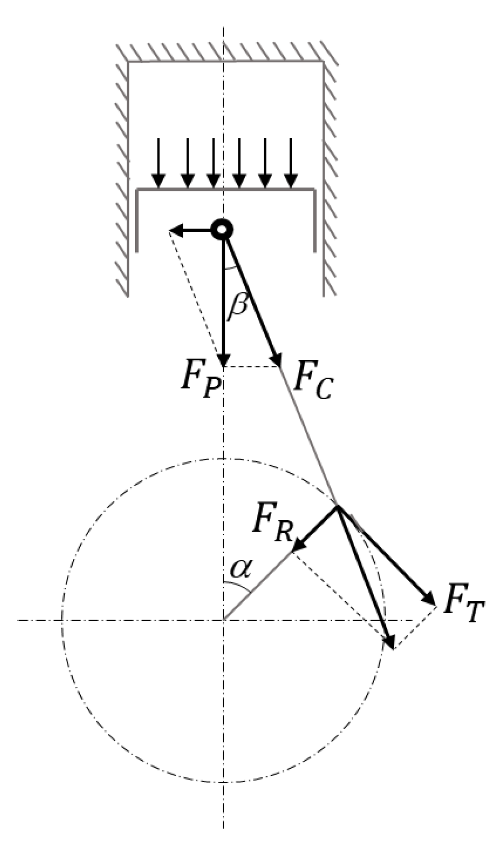
2. Theory
3. Modeling and Analysis
3.1. Engine Basic Parameters
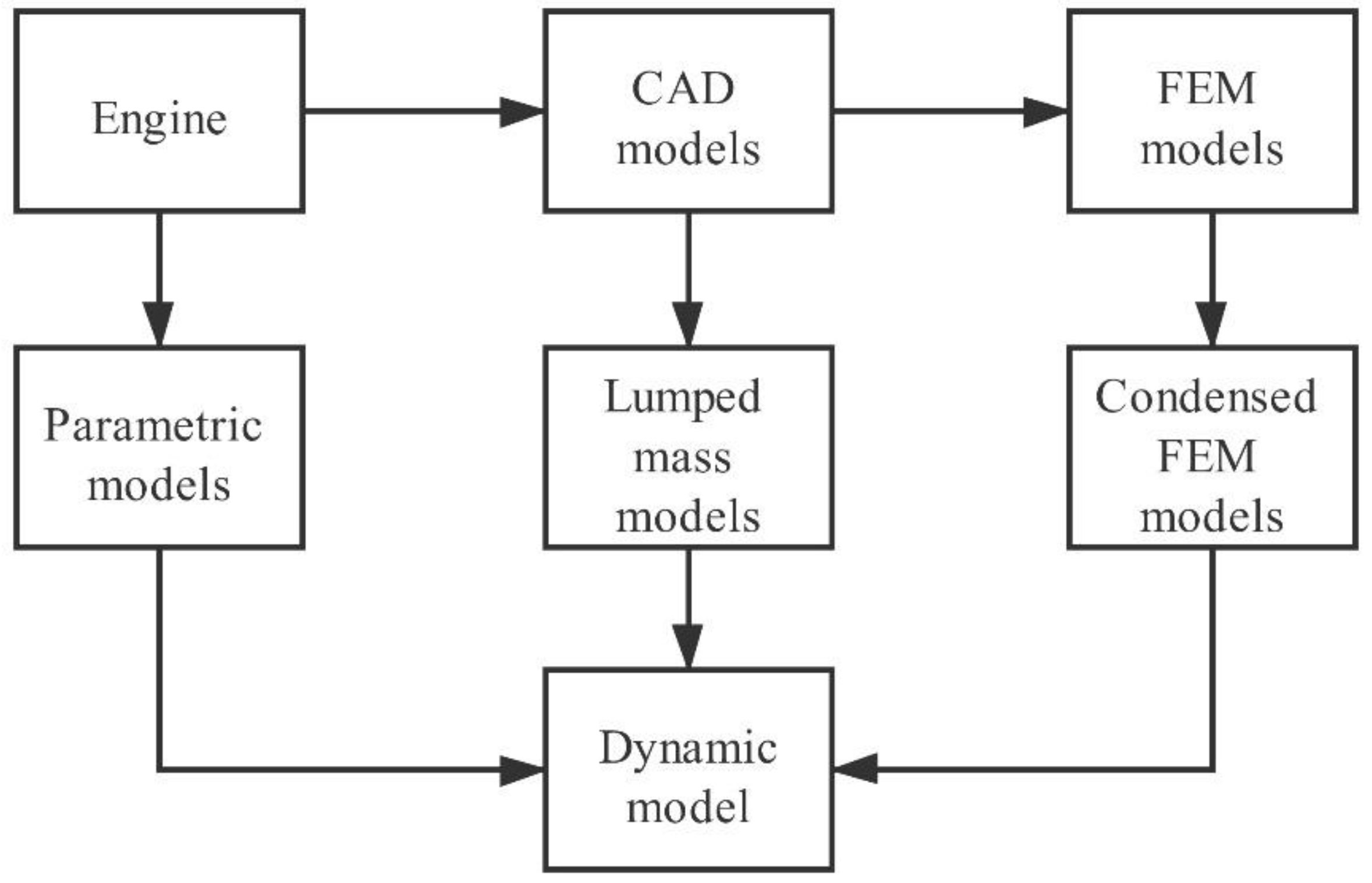
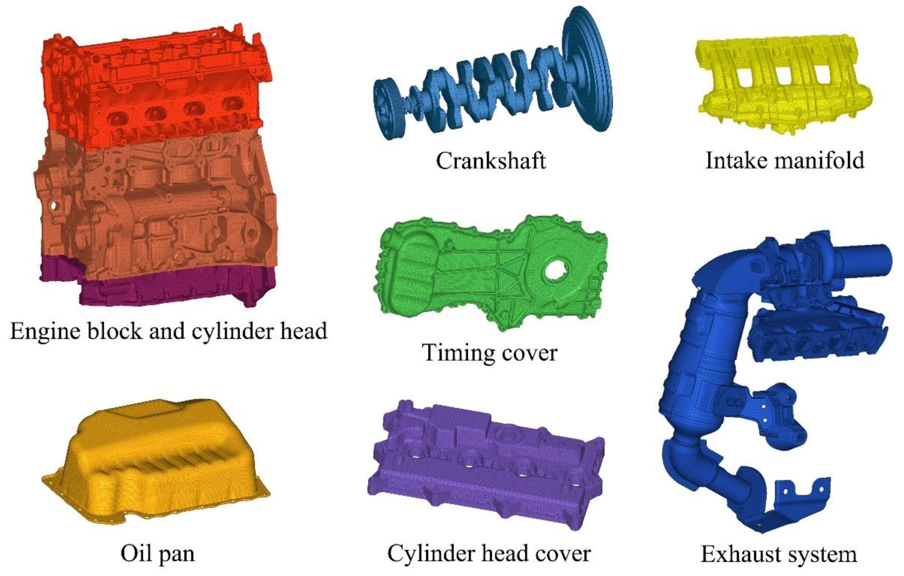
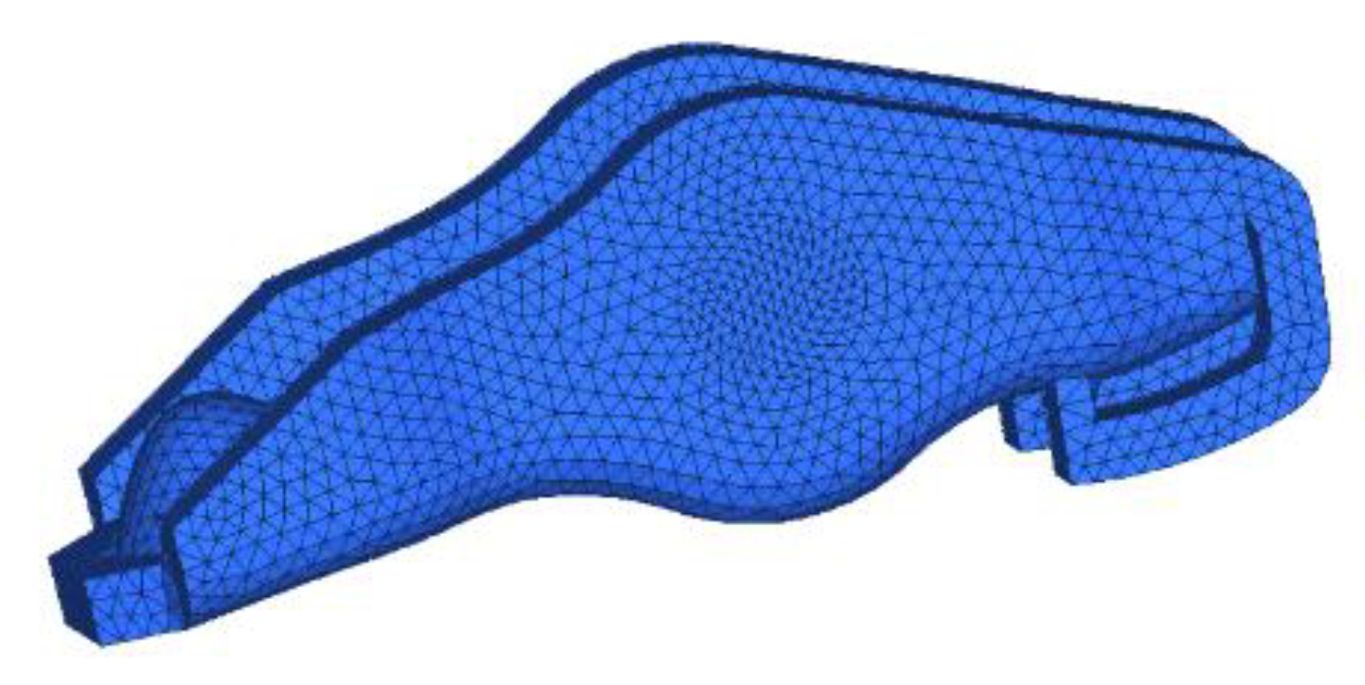
3.2. FEM Models
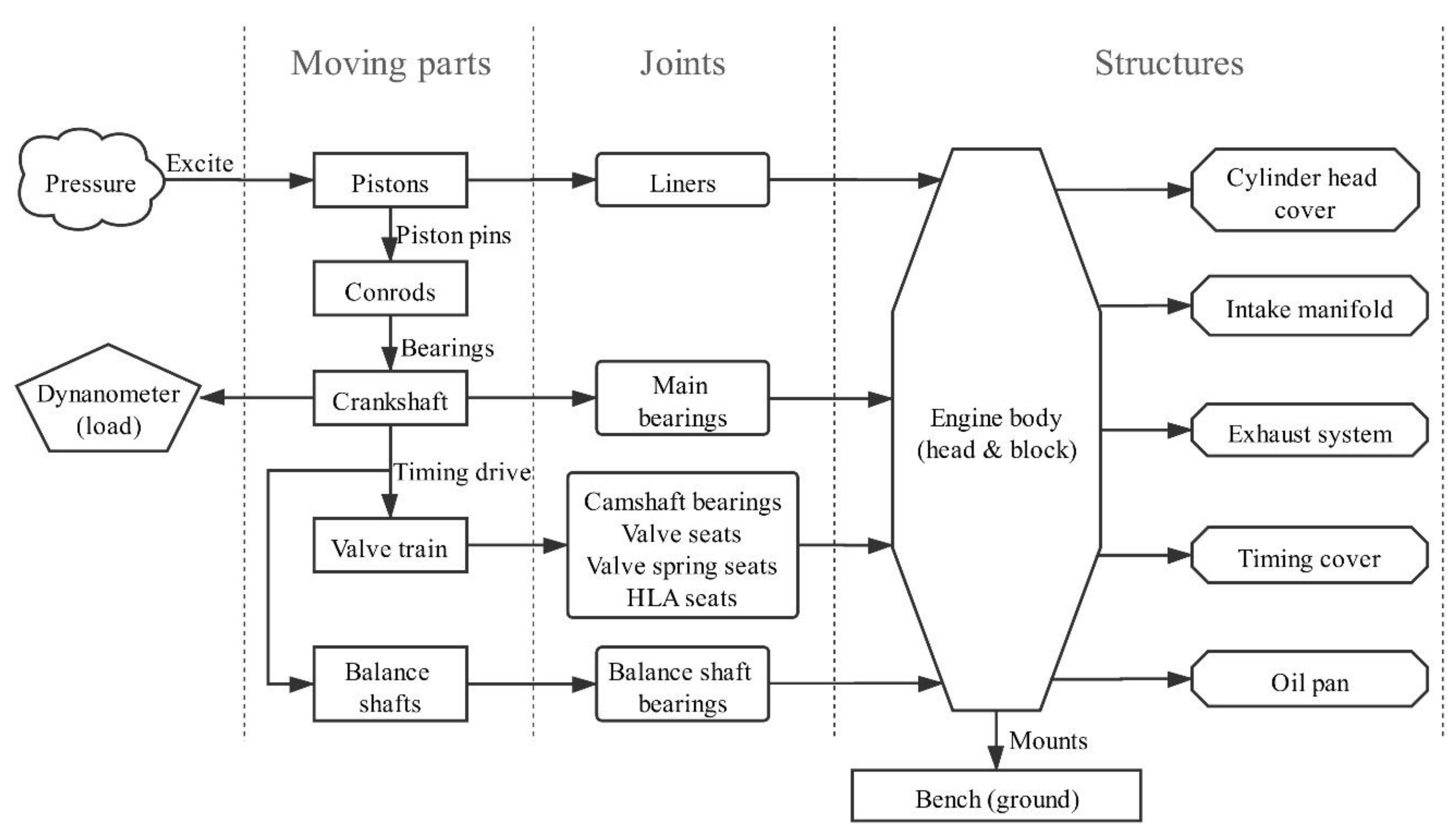
3.3. Multi-Body Dynamic Model
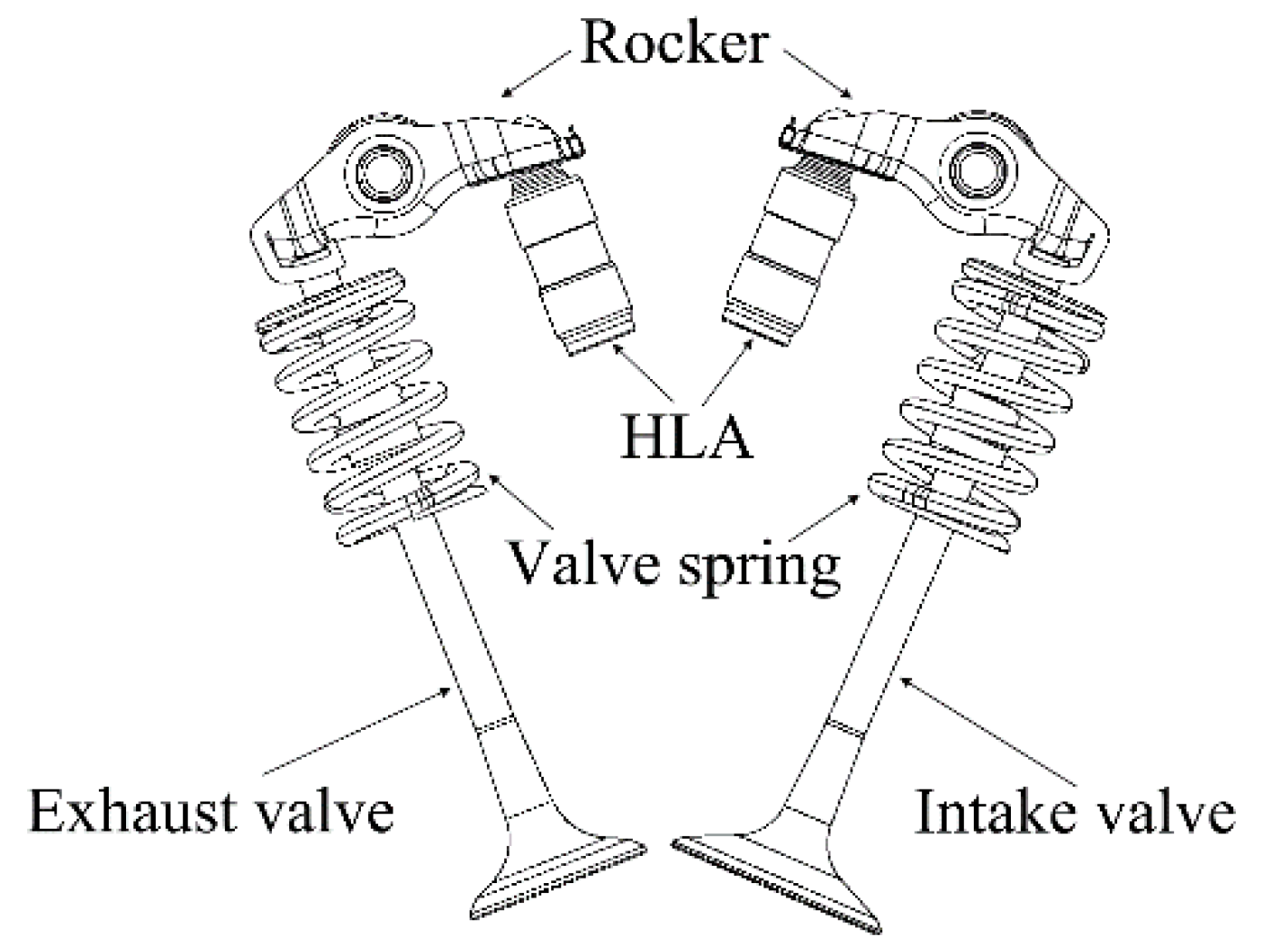
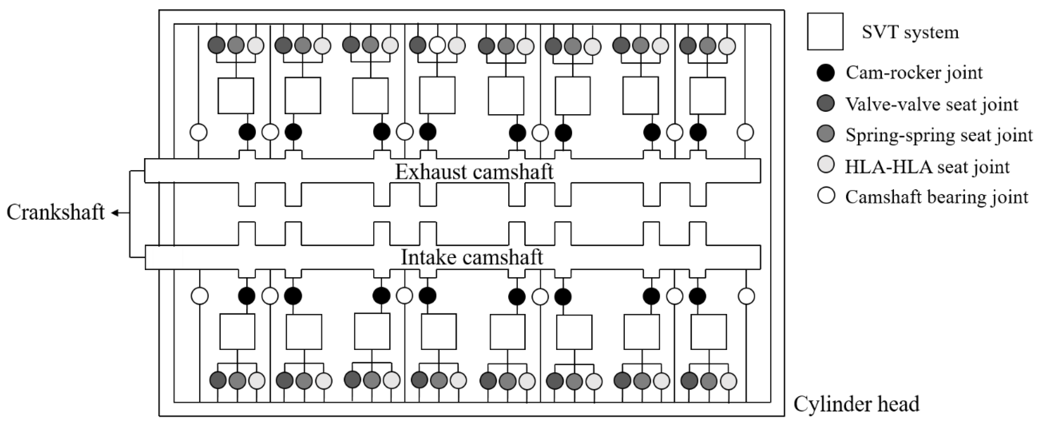
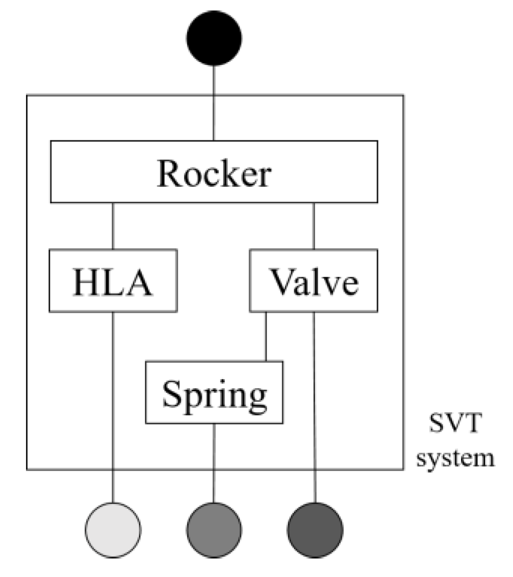
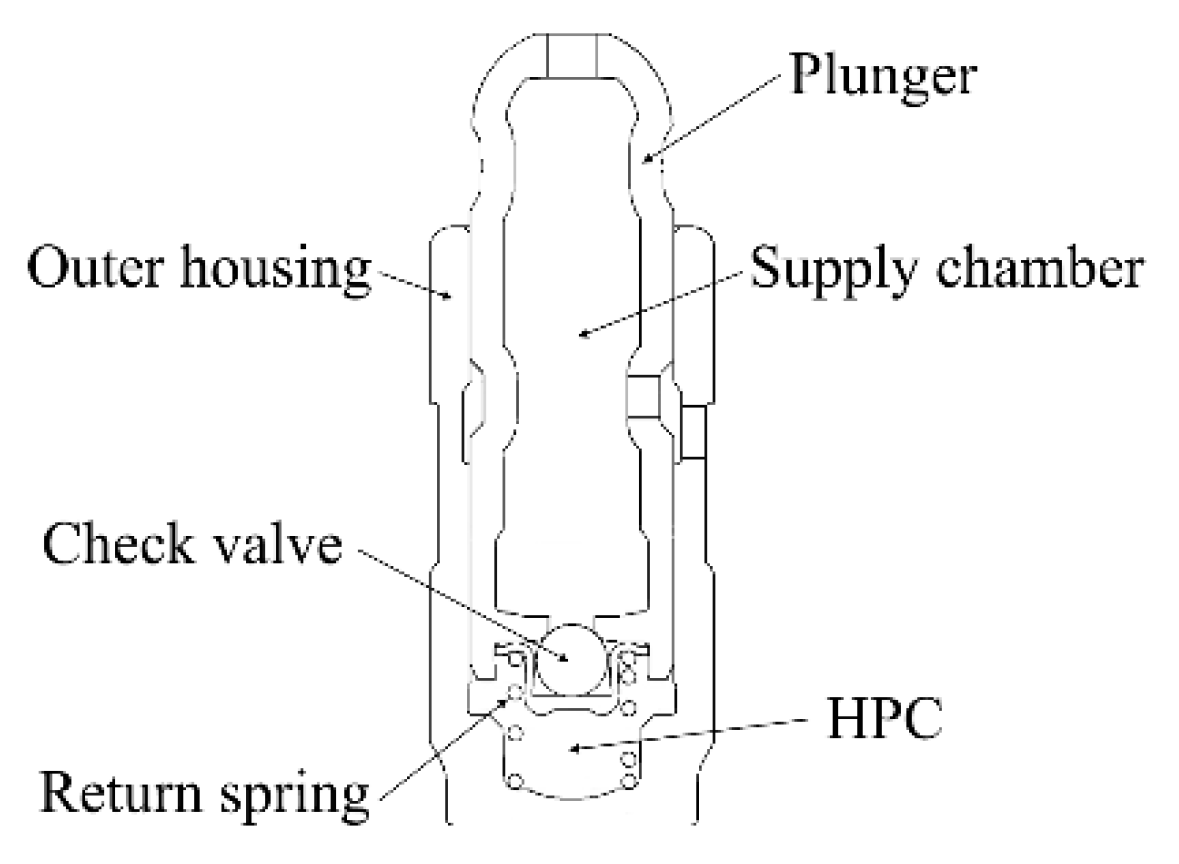
3.4. Valve Train System Model
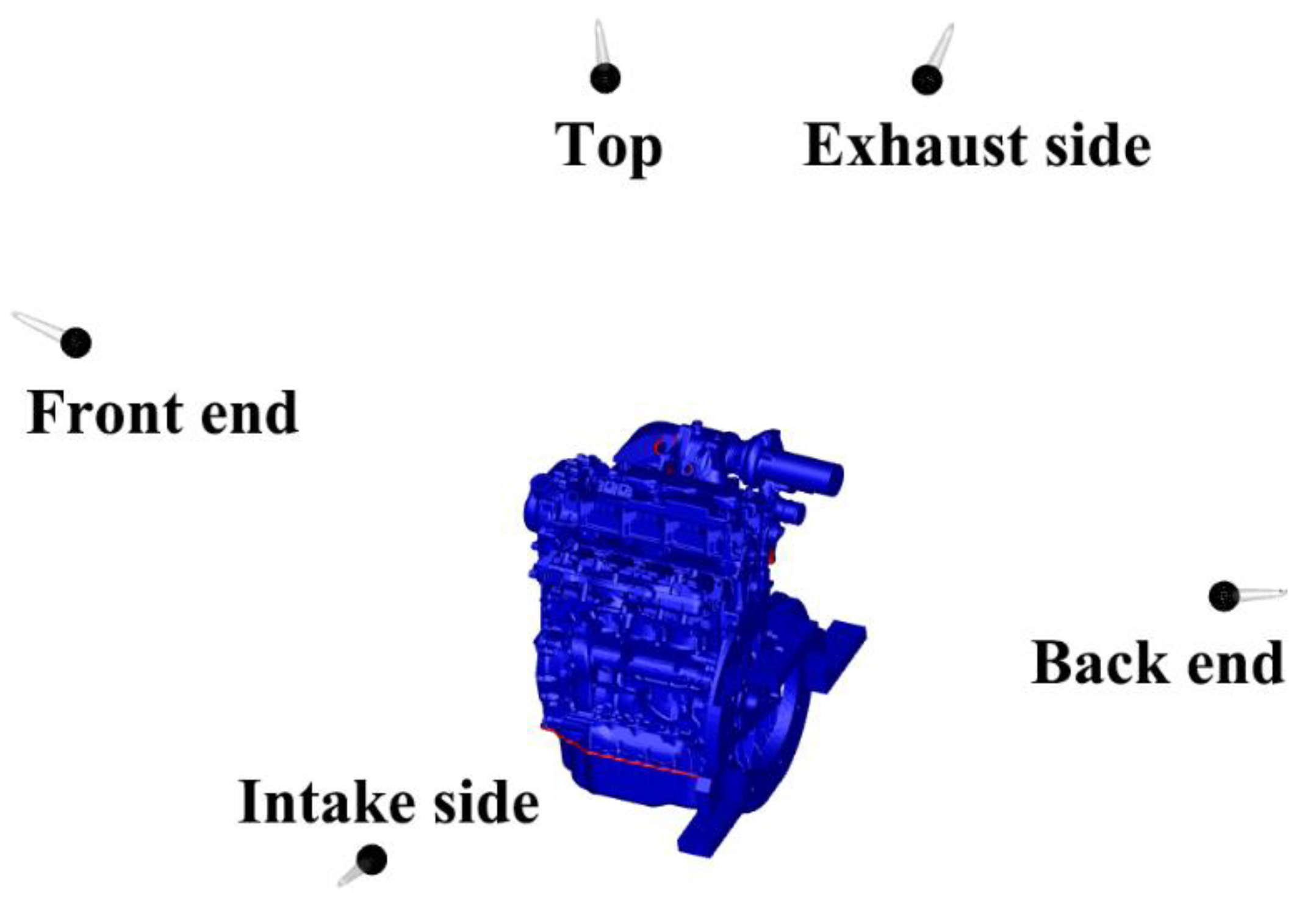
3.5. Acoustic Model
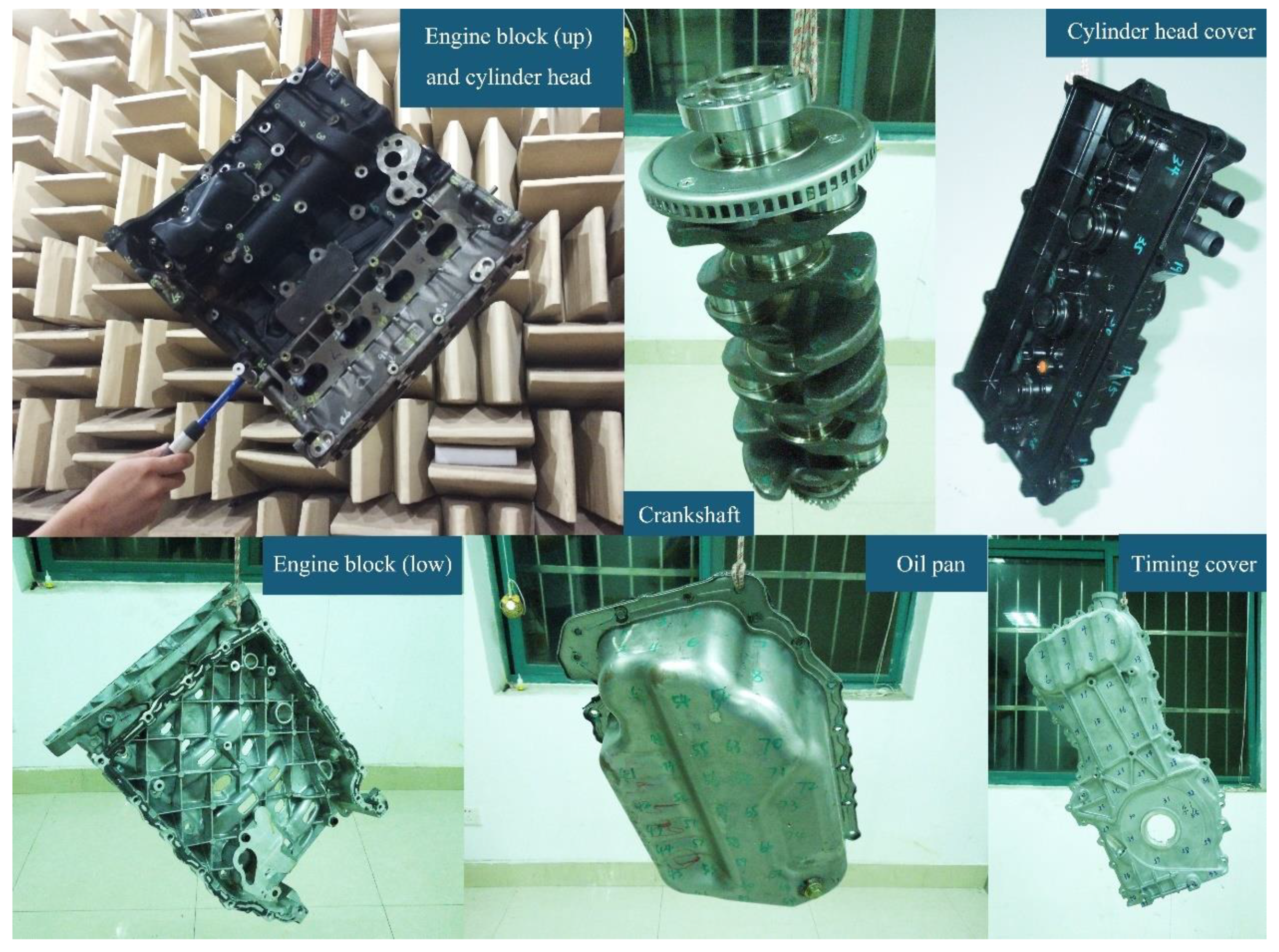
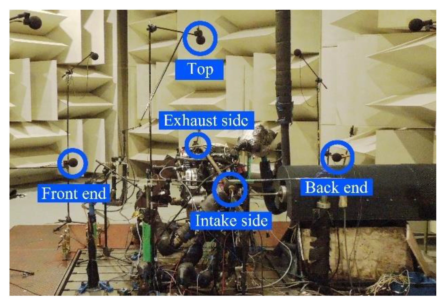
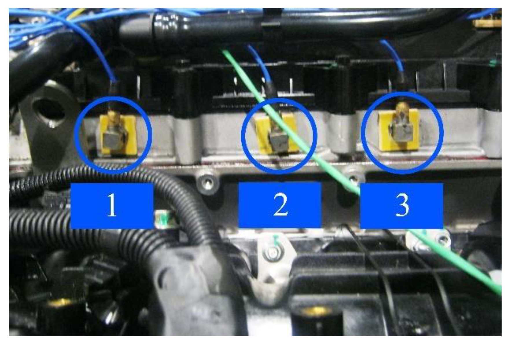
4. Experimental Setup
5. Results and Discussion
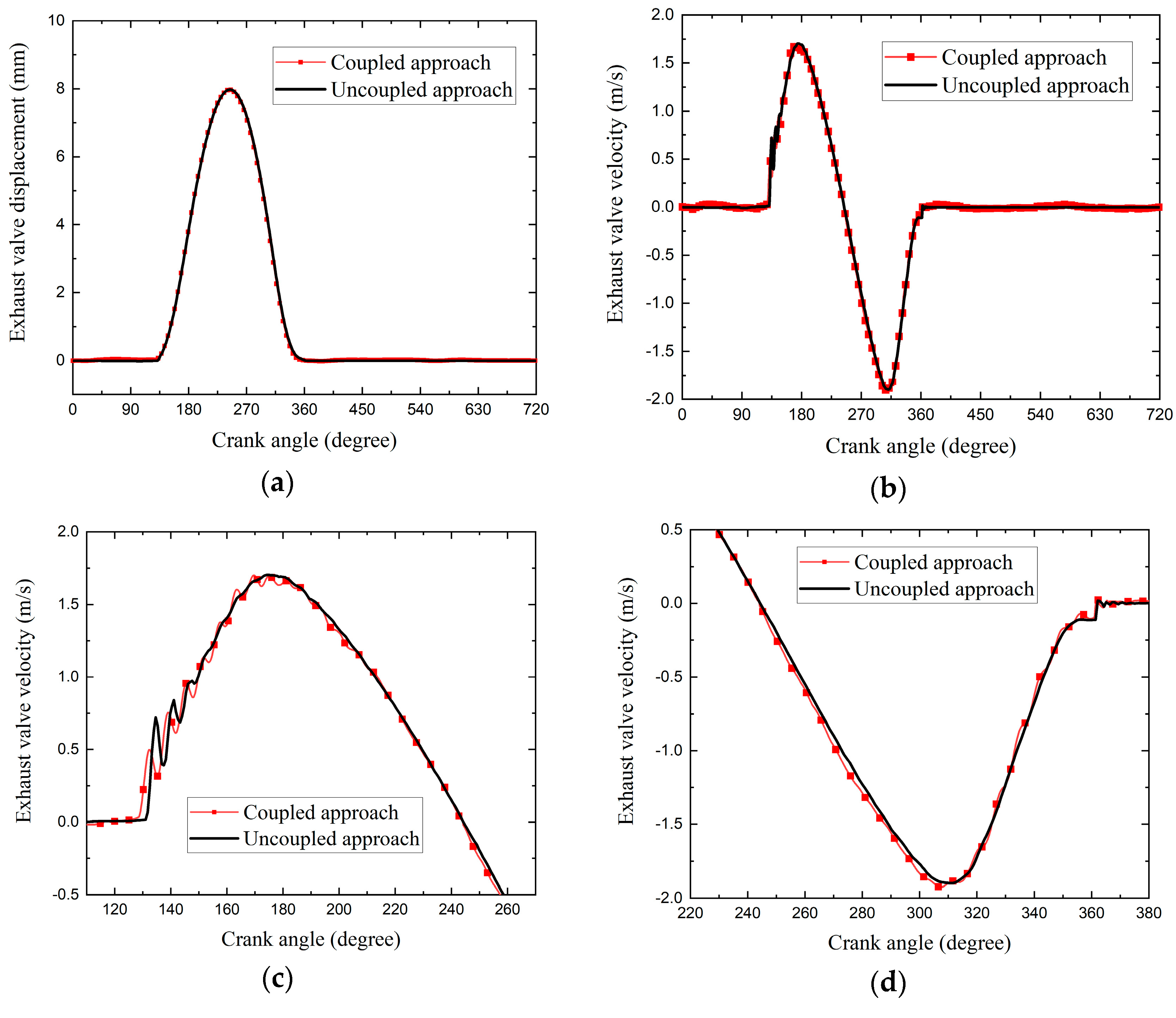
5.1. Valve Train Dynamic Analysis
5.2. Vibration and Noise Results Analysis
6. Conclusions
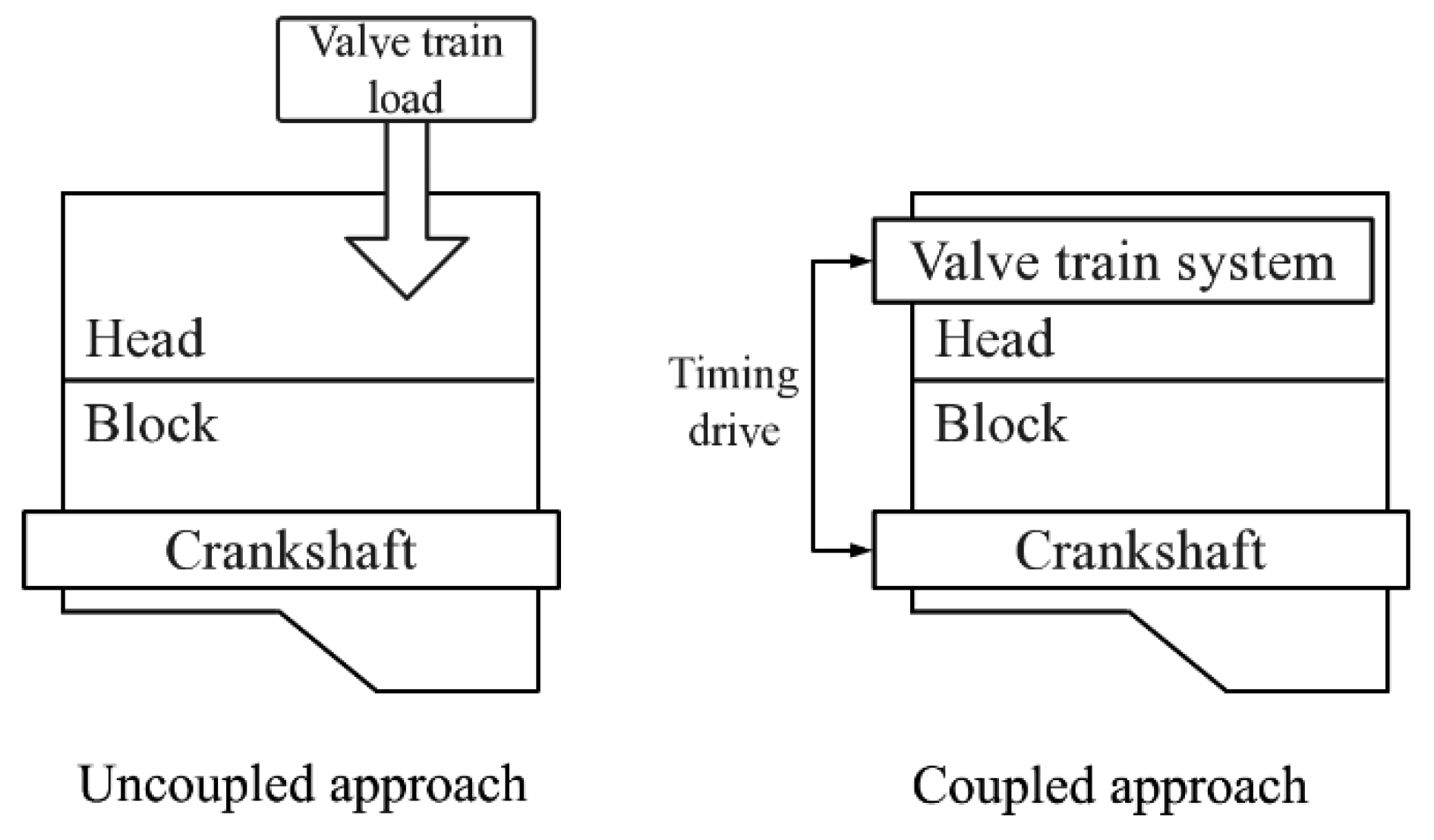
- The coupled approach considers interaction ignored in the uncoupled approach, which can improve the fidelity of the model. The impact of the cylinder head deformation to the valve train and the support and constraints of the valve train on the cylinder head are taken into consideration in the coupled approach. The camshaft speed is obtained from the crankshaft speed in the simulation, instead of a constant or preset speed. Therefore, the influence of speed fluctuation on the valve train is taken into consideration as well.
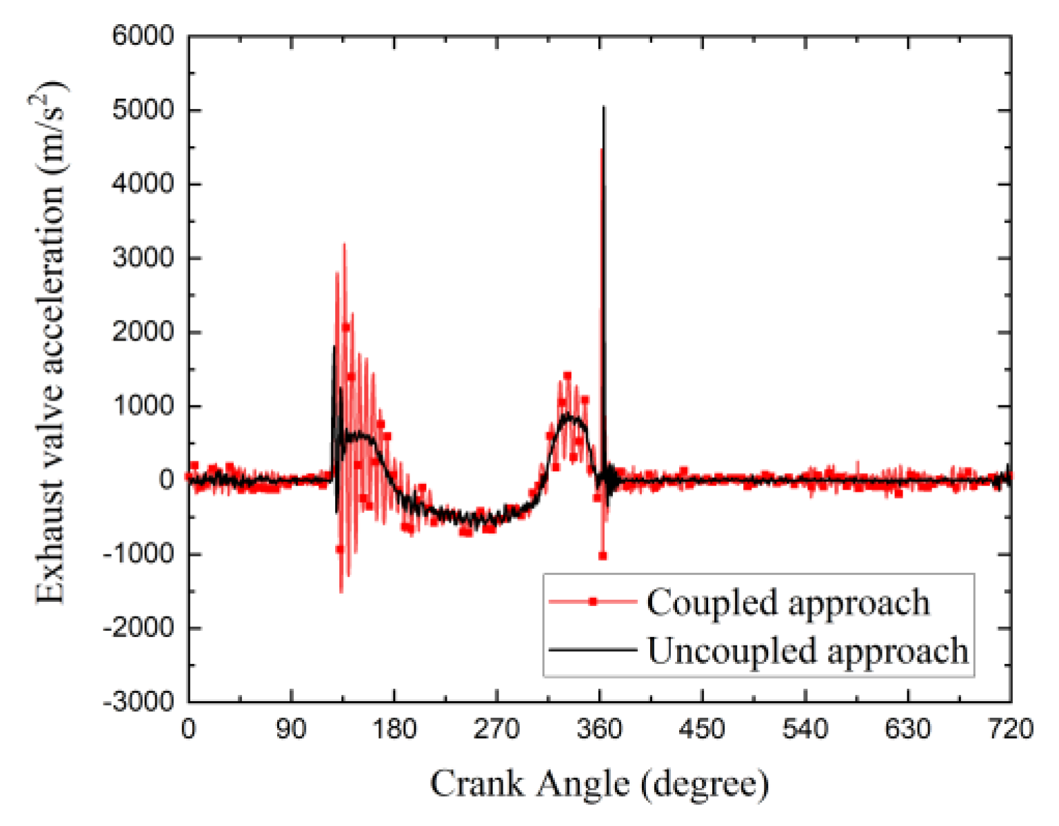
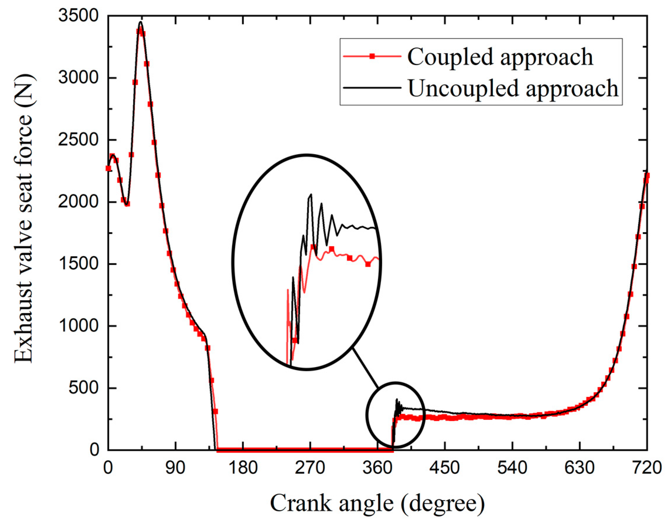
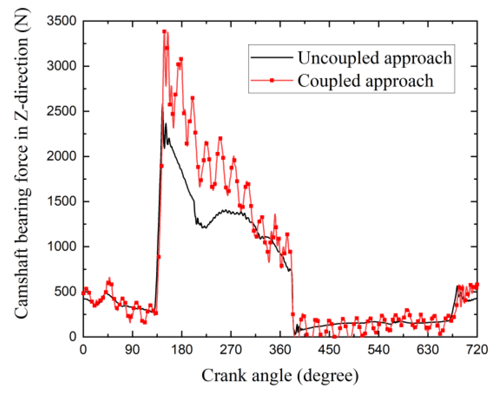
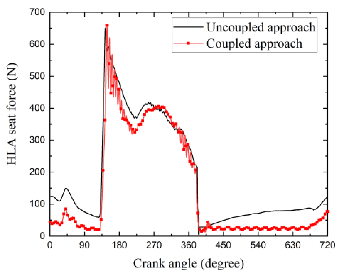
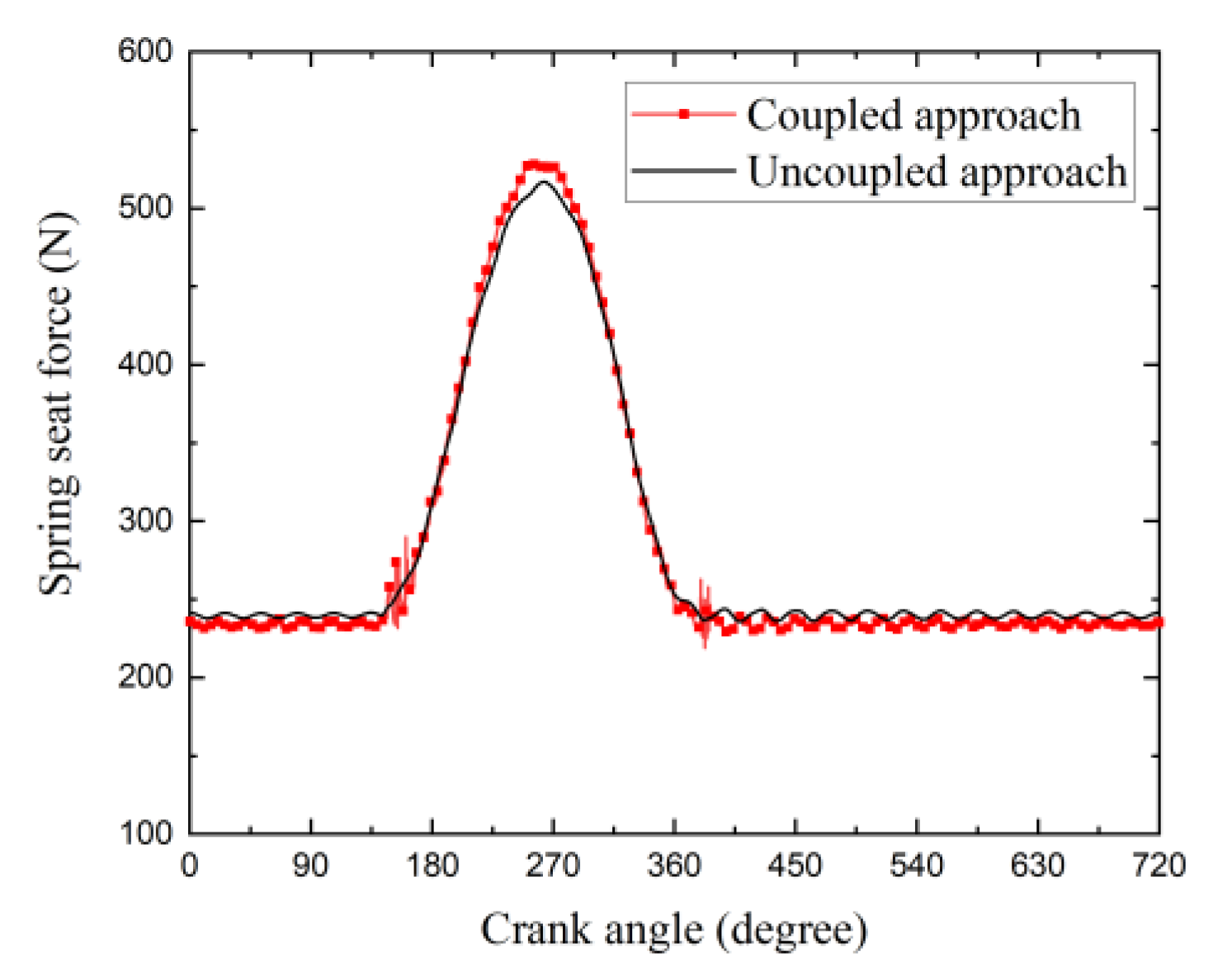
- Applying the coupled approach, more detailed dynamic results of the valve train are presented. The influence of the interaction between the valve train system and the cylinder head can be observed in the simulation results of the parts displacements, velocities, accelerations, and forces. The coupled approach is more instructive for analyzing the fatigue problems and abnormal noise problems of the valve train system.
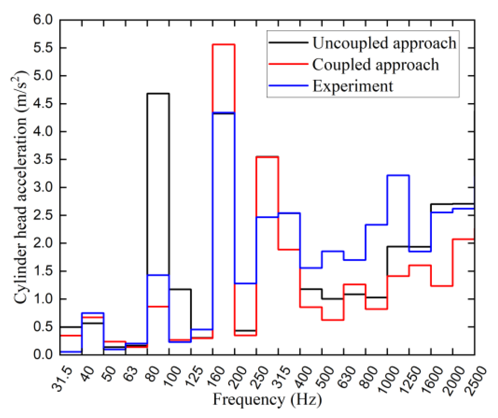
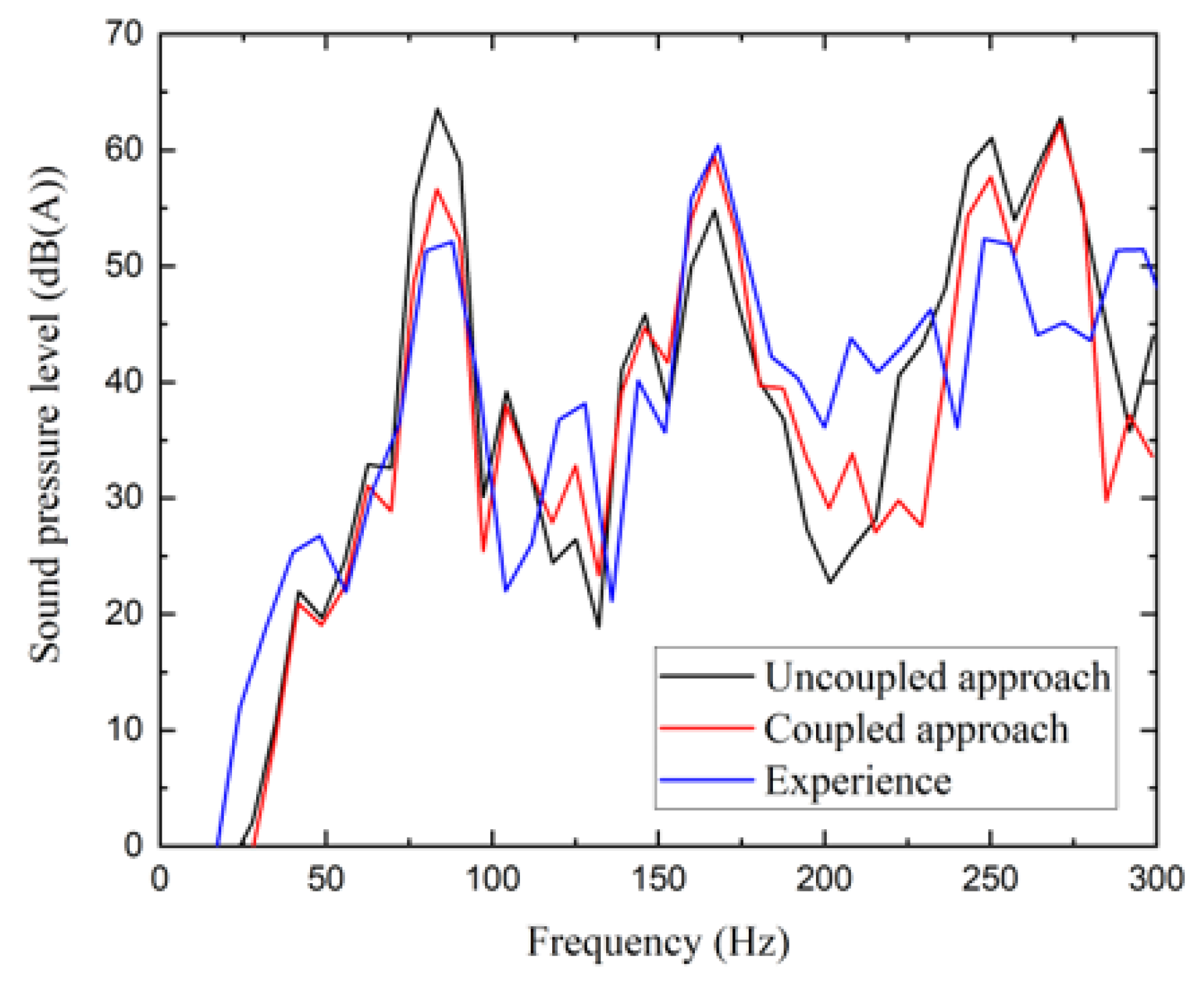
- Compared with the uncoupled approach, the results of the coupled approach have a better accuracy in vibration simulations. The vibration of the cylinder head measuring point at the second-order frequency (83.3 Hz) is severely overestimated in the uncoupled approach, resulting in the overestimation of the overall vibration and noise. In the coupled approach, the results of vibration at the second-order frequency are closer to the experimental values.
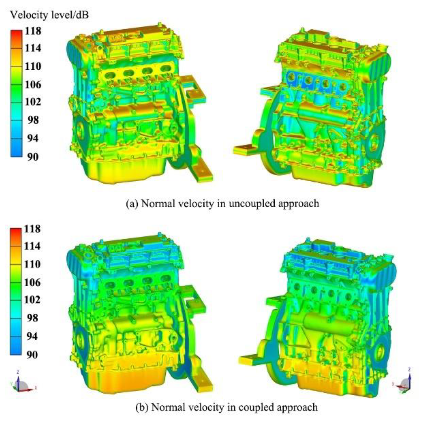
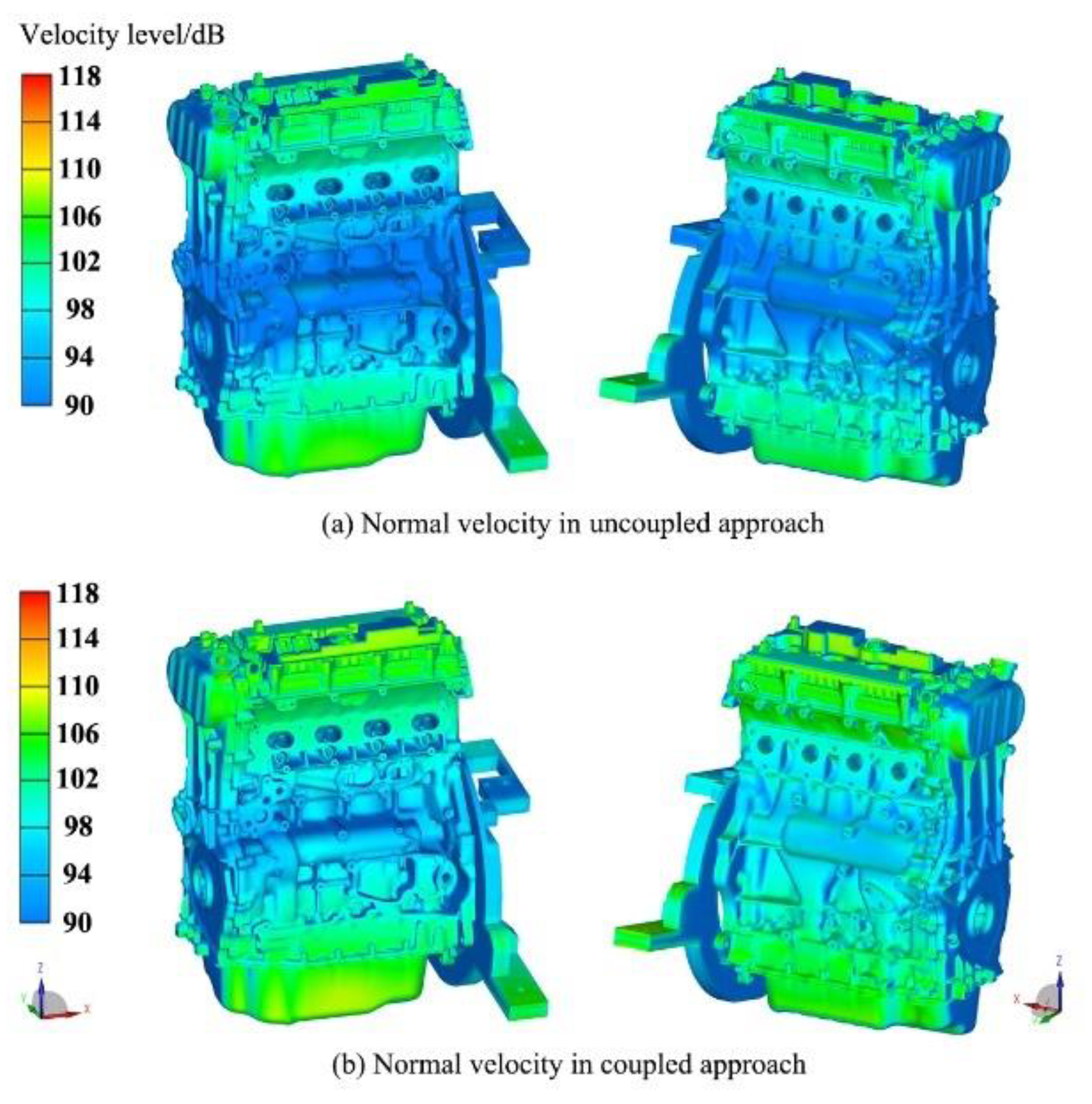
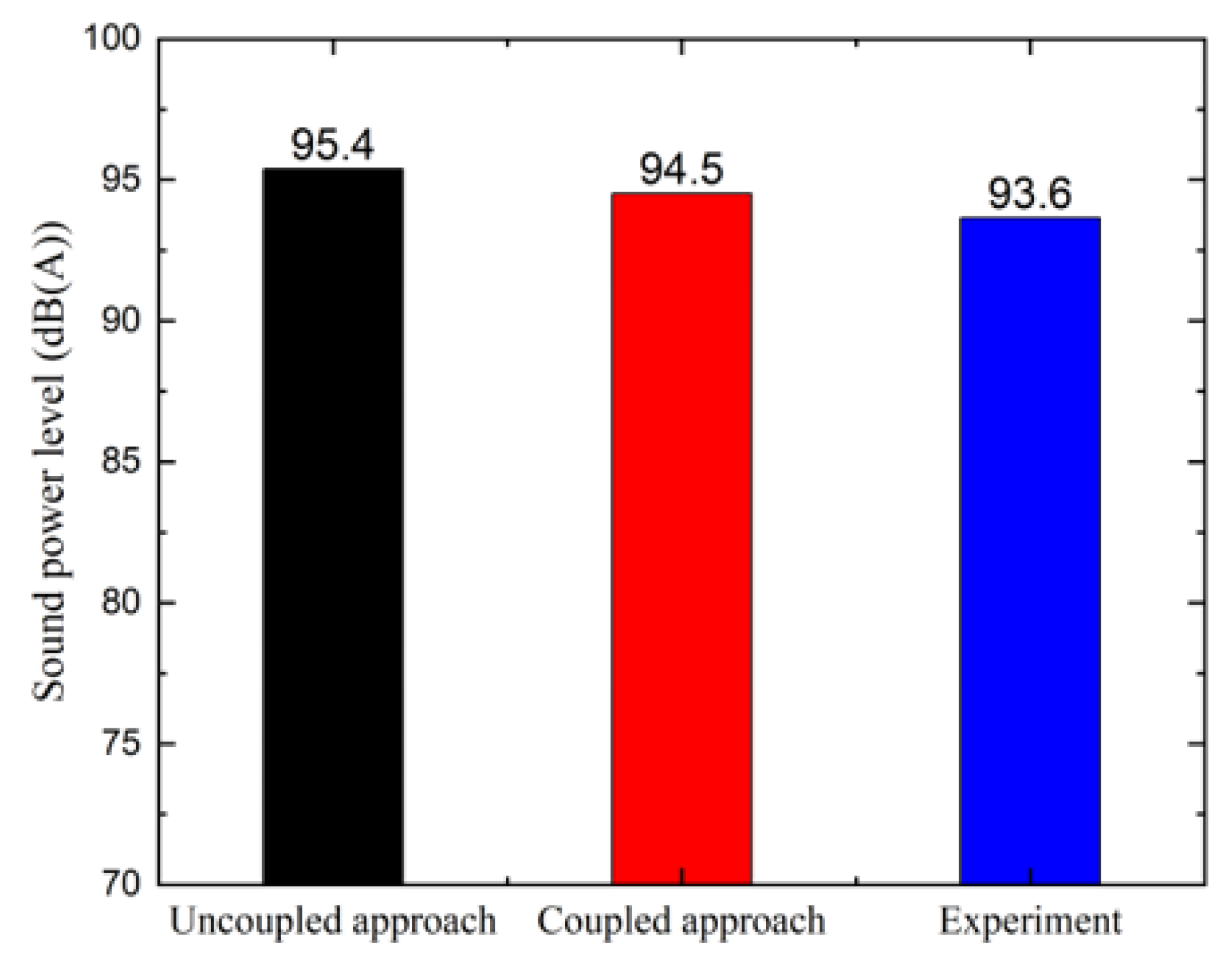
- The coupled approach has a better accuracy in noise prediction as well. The calculated overall sound power level values in the uncoupled and coupled approaches are 95.4 dB(A) and 94.5 dB(A), respectively, while the experimental value is 93.6 dB(A). After using the coupled approach, the difference from the experimental value is reduced from 1.8 dB(A) to 0.9 dB(A).
Author Contributions
Funding
Conflicts of Interest
References
- Dudley, W.M. New method in valve cam design. SAE Tech. Pap. 1948, 480170. [Google Scholar] [CrossRef]
- Eiss, N.S., Jr. Vibration of cams having two degrees of freedom. J. Eng. Ind. 1964, 86, 343–349. [Google Scholar] [CrossRef]
- Chan, C. Dynamic model of a fluctuating rocker-arm ratio cam system. J. Mech. Des. 1987, 109, 356–365. [Google Scholar] [CrossRef]
- Seidlitz, S. Valve train dynamics-a computer study. SAE Tech. Pap. 1989, 890620. [Google Scholar] [CrossRef]
- Nagaya, K. Vibration analysis of high rigidity driven valve system of internal combustion engines. J. Sound Vib. 1993, 165, 31–43. [Google Scholar] [CrossRef]
- Pisano, A.P. An experimental and analytical investigation of the dynamic response of a high-speed cam-follower system. J. Mech. Transm. Autom. Des. 1983, 105, 699–704. [Google Scholar] [CrossRef]
- Lassaad, W. Nonlinear dynamic behaviour of a cam mechanism with oscillating roller follower in presence of profile error. Front. Mech. Eng. 2013, 8, 127–136. [Google Scholar] [CrossRef]
- Guo, J. A new numerical method for developing the lumped dynamic model of valve train. J. Eng. Gas Turbines Power 2015, 137, 101507. [Google Scholar] [CrossRef]
- Zhou, C. An enhanced flexible dynamic model and experimental verification for a valve train with clearance and multi-directional deformations. J. Sound Vib. 2017, 410, 249–268. [Google Scholar] [CrossRef]
- Meuter, M. Multi-Body engine simulation including elastohydrodynamic lubrication for non-conformal conjunctions. Proc. Inst. Mech. Eng. Part K J. Multi-Body Dyn. 2017, 231, 457–468. [Google Scholar] [CrossRef]
- Offner, G. Modelling of condensed flexible bodies considering non-linear inertia effects resulting from gross motions. Proc. Inst. Mech. Eng. Part K J. Multi-Body Dyn. 2011, 225, 204–219. [Google Scholar] [CrossRef]
- Angeles, J.; Zakhariev, E. Computational Methods in Mechanical Systems: Mechanism Analysis, Synthesis, and Optimization; Springer: Berlin/Heidelberg, Germany, 1998. [Google Scholar]
- Morrison, D. A framework for modal synthesis. Comput. Music J. 1998, 17, 45–56. [Google Scholar] [CrossRef]
- Craig, R.R., Jr.; Bampton, M.C.C. Coupling of substructures for dynamic analyses. AIAA J. 1968, 6, 1313–1322. [Google Scholar] [CrossRef]
- Liu, R. A study of the influence of cooling water on the structural modes and vibro-acoustic characteristics of a gasoline engine. Appl. Acoust. 2016, 104, 42–49. [Google Scholar] [CrossRef]
- Teodorescu, M. Multi-Physics analysis of valve train systems: From system level to microscale interactions. Proc. Inst. Mech. Eng. Part K J. Multi-Body Dyn. 2007, 221. [Google Scholar] [CrossRef]
- Haslinger, J. Non-Smooth dynamics of coil contact in valve springs. J. Appl. Math. Mech. 2014, 94, 957–967. [Google Scholar] [CrossRef]
- Beloiu, D.M. Modeling and analysis of valve train, part I-conventional systems. SAE Int. J. Engines 2010, 3, 850–877. [Google Scholar] [CrossRef]
- ISO. Acoustics—Determination of Sound Power Levels and Sound Energy Levels of Noise Sources Using Sound Pressure—Engineering Methods for an Essentially Free Field Over a Reflecting Plane; International Organization Standardization: Geneva, Switzerland, 2010; Volume 3744. [Google Scholar]
- Desmet, W. A Wave Based Prediction Technique for Coupled Vibro-Acoustic Analysis. Ph.D. Thesis, Katholieke Universiteit Leuven, Leuven, Belgium, 1998. [Google Scholar]
- AVL Workspace. Excite-Power-Unit Theory: AVL User Manuals. 2017. Available online: http://www.avl-ast-china.com/upload/ueditor/file/20170516/1494905319788032969.pdf (accessed on 24 July 2020).
- Andreatta, E.C. Valve train kinematics and dynamics simulation. SAE Tech. Pap. 2016, 36, 0213. [Google Scholar] [CrossRef]


| Engine type | Four cylinders four strokes gasoline engine |
| Intake type | Turbocharged |
| Displacement | 1798 cc |
| Bore | 82.5 mm |
| Stroke | 84.2 mm |
| Max power | 120 kW@5500 rpm |
| Max torque | 250 Nm@1500–4500 rpm |
| Balance | Double balancing shaft |
| Valve train | DOHC |
| End-pivot rocker arm (roller finger follower) | |
| HLA |
| Elements | Material | Density (g/cm3) | Young’s Modulus (MPa) | Poisson’s Ratio | |
|---|---|---|---|---|---|
| Crankshaft | 93,196 | Steel | 7.85 | 210,000 | 0.30 |
| Oil pan | 9043 | ||||
| Block | 269,359 | Cast iron | 7.30 | 110,000 | 0.30 |
| Cylinder head | 139,218 | Aluminum alloy | 2.73 | 76,550 | 0.34 |
| Timing cover | 91,996 | ||||
| Cylinder head cover | 64,609 | Polypropylene | 1.40 | 3150 | 0.35 |
| Intake manifold | 166,391 | Polyamide | 1.50 | 1800 | 0.30 |
| Exhaust system | 98,330 | Cast iron | 7.80 | 191,000 | 0.30 |
| Components | Order | Simulation/Hz | Measurement/Hz | Error |
|---|---|---|---|---|
| Engine block (up) and cylinder head | 1 | 545.5 | 543.6 | 0.3% |
| 2 | 987.3 | 1042.0 | −5.2% | |
| 3 | 1368.2 | 1435.9 | −4.7% | |
| 4 | 1455.3 | 1488.6 | −2.2% | |
| 5 | 1635.9 | 1673.8 | −2.3% | |
| Engine block (low) | 1 | 327.5 | 309.8 | 5.7% |
| 2 | 793.3 | 790.9 | 0.3% | |
| 3 | 940.5 | 969.9 | −3.0% | |
| 4 | 1182.8 | 1145.3 | 3.3% | |
| 5 | 1461.8 | 1385.9 | 5.5% | |
| Crankshaft | 1 | 406.5 | 309.6 | 4.1% |
| 2 | 553.5 | 529.8 | 4.4% | |
| 3 | 907.9 | 881.0 | 3.1% | |
| 4 | 950.9 | 920.9 | 3.3% | |
| 5 | 961.6 | 923.3 | 4.2% | |
| Cylinder head cover | 1 | 128.5 | 133.2 | −3.5% |
| 2 | 204.1 | 201.7 | 1.2% | |
| 3 | 348.6 | 346.6 | 0.6% | |
| 4 | 386.6 | 401.1 | 3.6% | |
| 5 | 439.6 | 435.8 | 0.9% | |
| Timing cover | 1 | 197.6 | 194.3 | 1.7% |
| 2 | 255.6 | 250.6 | 2.0% | |
| 3 | 539.4 | 531.5 | 1.5% | |
| 4 | 692.3 | 678.9 | 2.0% | |
| 5 | 812.9 | 804.1 | 1.1% | |
| Oil pan | 1 | 193.4 | 197.7 | −2.2% |
| 2 | 323.1 | 329.5 | −1.7% | |
| 3 | 502.7 | 490.9 | 2.4% | |
| 4 | 572.0 | 578.1 | −1.1% | |
| 5 | 775.8 | 807.4 | −3.9% |
© 2020 by the authors. Licensee MDPI, Basel, Switzerland. This article is an open access article distributed under the terms and conditions of the Creative Commons Attribution (CC BY) license (http://creativecommons.org/licenses/by/4.0/).
Share and Cite
Zheng, X.; Luo, X.; Qiu, Y.; Hao, Z. Modeling and NVH Analysis of a Full Engine Dynamic Model with Valve Train System. Appl. Sci. 2020, 10, 5145. https://doi.org/10.3390/app10155145
Zheng X, Luo X, Qiu Y, Hao Z. Modeling and NVH Analysis of a Full Engine Dynamic Model with Valve Train System. Applied Sciences. 2020; 10(15):5145. https://doi.org/10.3390/app10155145
Chicago/Turabian StyleZheng, Xu, Xuan Luo, Yi Qiu, and Zhiyong Hao. 2020. "Modeling and NVH Analysis of a Full Engine Dynamic Model with Valve Train System" Applied Sciences 10, no. 15: 5145. https://doi.org/10.3390/app10155145
APA StyleZheng, X., Luo, X., Qiu, Y., & Hao, Z. (2020). Modeling and NVH Analysis of a Full Engine Dynamic Model with Valve Train System. Applied Sciences, 10(15), 5145. https://doi.org/10.3390/app10155145