A Multicriteria Motion Planning Approach for Combining Smoothness and Speed in Collaborative Assembly Systems

Abstract

Human–robot interaction is an important aspect of Industry 4.0, and the extended use of robotics in industrial environments will not be possible without enabling them to safely interact with humans. This imposes relevant constraints in the qualitative characterization of the motions of robots when sharing their workspace with humans. In this paper, we address the trade-off between two such constraints, namely the smoothness, which is related to the cognitive stress that a person undergoes when interacting with a robot, and the speed, which is related to normative safety requirements. Given an execution time, such an approach will allow us to plan safe trajectories without neglecting cognitive ergonomics and production efficiency aspects. We first present the methodology able to express the balance between these qualities in the form of a composite objective function. Thanks to the variational formalism, we identify the related set of optimal trajectories with respect to the given criterion and give a suitable parametrization to them. Then, we are able to formulate the safety requirements in terms of a reparametrization of the motion. Finally, numerical and experimental results are provided. This allows the identification of the preferable sets of the possible motions that satisfy the operator’s psychological well-being and the assembly process performance by complying with the safety requirements in terms of mechanical risk prevention.

1. Introduction

Collaborative robots (cobots) are robots designed to enable the combination of the strength, force, and repeatability of automatic machines with the dexterity and cognitive capacities of humans, allowing them to work together in a shared workspace. It is expected that they will boost the Industry 4.0 revolution and, in particular, the digitalization and the human-centered design of an industrial workspace [1].

However, the physical human–robot interaction (pHRI) required in such a shared workspace introduces novel mechanical risks with respect to “traditional” industrial robots [2]. In this regard, the International Organisation for Standardization (ISO) has introduced four methods of operation [2]: i.e., hand guiding, safety-rated monitored stop, speed and separation monitoring, and power and force limiting. Such modalities constitute a framework to define a cobot, proposing proper implementations and evaluations of safety requirements in terms of mechanical risk.

Commercially available solutions provide out-of-the-box user interfaces and tunable parameters to allow the integrator to implement these collaborative operation methods [3,4,5].

In addition to safety, other important topics that have to be considered when designing and implementing a collaborative workspace are physical and cognitive ergonomics. For the former, we can utilize industry standards, guidelines, and best practices already developed for manual work and modify and apply them to collaborative scenarios [6,7]. On the contrary, the latter has not yet been fully studied, and guidelines and best practices are not available [8].

It has been demonstrated that the operator’s subjective acceptance of pHRI can be increased by means of smooth, i.e., predictable, motions [9,10,11,12]. We therefore formulate a robot motion planning approach to achieve a psychologically less-stressful working environment.

Among all motion planning techniques that are available in the literature, trajectory planning through via-points is of particular importance for collaborative robotics. The Technical Specification ISO TS-15066 [13] foresees the hand guiding modality as collaborative operation: even unskilled workers can intuitively program a path by simply moving the robot manually in its workspace and saving step-by-step the needed via-points through an interface. The worker can thus directly define the robot’s configuration and avoid the obstacles that may be placed in the reachable workspace. The computation of a safe trajectory along the via-points is then made by the robot controller according to the ISO specifications.

Starting from the outcome of the hand-guiding operation and path definition, this work focuses on the problem of designing trajectories that allow guaranteeing both safe and psychologically less stressful movements without overlimiting the robot performance.

In the literature, there is a plethora of different techniques for planning a robotic trajectory [14] that focus on the optimization/minimization of, e.g., time, smoothness, energy, and torque. Among these, minimum jerk motion profiles have drawn particular interest in the robotics community for mainly two reasons:

• There is experimental evidence that suggests that humans adopt minimum jerk movements [15,16,17], and thus, these can be perceived as predictable and familiar by a person that interacts with the robot. In [18], the impact of different industrial robot motion profiles was investigated in a cooperative human-robot interaction (HRI) task showing that minimum jerk trajectories significantly reduce the heart rate in humans, thus suggesting an improvement of robot acceptance and a reduction of the psychological stress;
• Minimum-jerk trajectories reduce the induced mechanical vibrations and, thus, wear in the elements of an automatic machine, e.g., robot, as well as the error during the trajectory tracking phase [19,20,21,22,23,24].

Thus, we conclude that minimum jerk trajectories allow psychologically less stressful movements with respect to well-known ones like trapezoidal speed profiles. However, as pointed out by the authors in [25], minimum jerk motions could have two potential drawbacks that degrade the robot’s behavior:

• For a given execution time, minimum jerk motions could require higher speeds than trapezoidal speed profiles. To make the motion feasible for the robot and for the safety requirement, an upper bound value of velocity has to be set, and a linear scaling of the trajectory penalizes this kind of trajectory in terms of execution time much more than it does for trapezoidal speed profiles;
• Large deviations from the straight lines that join consecutive via-points may occur. The magnitude of such deviations is not predictable and may create unexpected deviations from the intended path between via-points, forcing the user to define additional via-points to possibly limit this problem.

In this paper, we overcome these issues by formulating a multi-criteria optimization problem in order to take into account both the jerk and the speed along the path that joins a sequence of via-points. Following the approach developed in [25], we directly apply the variational formalism to derive a family of trajectories that are parametrized with respect to a parameter that expresses the required balance. As a result, we obtain a human-friendly motion planning methodology, the input of which is given by the via-points introduced during the hand-guiding programming phase, and the output is a reference trajectory for the robot’s controller.

In Section 2, we formulate the problem of trajectory planning through via-points and demonstrate that the previously mentioned drawbacks of minimum jerk motions are consequences of a naturally large arc-length. Then, we formulate a multi-criteria (multi-objective) optimization problem that accounts for balance between arc-length and jerk. This section finishes with the application of the variational formalist to the proposed problem. In Section 3, we provide the means to implement this kind of motion in a collaborative environment, and we leverage a Pareto front to provide the user the necessary information to choose the balance parameter for the given execution time. Finally, in Section 4, the experimental results of the implemented trajectories are given.

2. Optimal Trajectory Formulation

2.1. General Problem Formulation

In order to exploit the benefits of a smooth, i.e., minimum jerk, trajectory, and limit the possible overshoots in the path, a trade-off method between the two objectives is investigated and proposed.

To obtain a uniform description of the motion regardless of the space in which the motion is planned, e.g., the joint space of a specific task, we describe it as a curve in an open subset $\Omega$ of an n-dimensional manifold $\mathcal{M}$ such that there exists a chart $(\psi ,\Omega )$ such that:

$$\mathit{\psi }:\Omega ⟶{\mathbb{R}}^n.$$

(1)

This allows identifying the motion with a curve in ${\mathbb{R}}^n$ without considering the specific details of the space where the planning is done.

Let us consider a partial description of a desired robot motion given as the execution time $t_f$ and an ordered sequence of $N+1$ via-points in the manifold.

Utilizing the previously introduced local coordinate map $\mathit{\psi }$, Equation (1), the problem can be rewritten in ${\mathbb{R}}^n$, and the ordered sequence of desired via-points can be described as $\mathit{VP}=\{{\mathbf{w}}_0,{\mathbf{w}}_1,\cdots ,{\mathbf{w}}_N\}\subset {\mathbb{R}}^n$.

This operation translates our problem into that of finding a reasonable curve joining the via-points $\mathit{VP}$ in such a way that the via-point ${\mathbf{w}}_i$ and the velocity ${\dot{\mathbf{w}}}_i$ are attained at the time $t_i$ with $t_i<t_{i+1}$ in which every instant $t_i$ is within the execution time interval $T=[0,t_f]$. Then, the position, velocity, and acceleration constraints can be written as:

$$\begin{array}{cc}\hfill \mathbf{q}\left(t_i\right)={\mathbf{w}}_i& \hfill \\ \hfill \dot{\mathbf{q}}\left(t_0\right)={\dot{\mathbf{w}}}_0& \hfill & \hfill \dot{\mathbf{q}}\left(t_N\right)={\dot{\mathbf{w}}}_N\\ \hfill \ddot{\mathbf{q}}\left(t_0\right)={\ddot{\mathbf{w}}}_0& \hfill & \hfill \ddot{\mathbf{q}}\left(t_N\right)={\ddot{\mathbf{w}}}_N.\end{array}$$

(2)

with $t_0=0$ and $t_N=t_f$.

We define the term reasonable curve as a curve that optimizes a desired cost function and is “physically” feasible. As the cost functions of this work include the integrals of the derivatives of $\mathbf{q}$, it is required that the k-th first derivatives are square integrable. Such a set of functions constitutes a Hilbert space, denoted by ${\mathbb{W}}^{2,k}(T,{\mathbb{R}}^n)$. The second requirement demands that $\mathbf{q}$ connects the via-points $\mathit{VP}$ with a trajectory that is continuous to the k-th order. Furthermore, such variations must be attainable by the dynamics of the systems.

Thus, we introduce the set of admissible motions as:

$$\mathcal{Q}=\left\{\mathbf{q}\in {\mathbb{W}}^{2,k}(T,{\mathbb{R}}^n)\cap C^k(T,{\mathbb{R}}^n)|\exists {\left\{t_i\right\}}_{i=0}^N\subset T\mathrm{s}.\mathrm{t}.\mathbf{q}\left(t_i\right)={\mathbf{w}}_i\mathrm{and}{t}_i<t_{i+1}\right\}.$$

(3)

The problem can then be seen as the one of finding the curve among the admissible motions $\mathcal{Q}$ such that a given performance index is minimized and additional possible constraints are satisfied.

We define the performance index as a map $I:\mathcal{Q}⟶\mathbb{R}$ that describes a desired quality of the motion under analysis by associating it with a real number. A simple way to construct such a performance index is to take the average value of a given scalar function F, which depends on the desired i-th derivative. The cost function I can then be expressed as:

$$I\left(\mathbf{q}\right)={\int }_0^{t_f}F(\mathbf{q},\dot{\mathbf{q}},\ddot{\mathbf{q}},\stackrel{⃛}{\mathbf{q}})\mathsf{d}t$$

(4)

We can then express the optimal trajectory planning problem in the following form:

$$\begin{array}{c}\hfill \begin{array}{cc}\hfill & \underset{\mathbf{q}}{min}I\left(\mathbf{q}\right)\hfill \\ \hfill & \mathrm{s}.\mathrm{t}.\mathbf{q}\in \mathcal{Q}.\hfill \end{array}\end{array}$$

(5)

to which further constraints can be added. The design problem is therefore often formulated in terms of minimum velocity $F=\parallel \dot{\mathbf{q}}\parallel$, minimum acceleration $F=\parallel \ddot{\mathbf{q}}\parallel$, and/or minimum jerk $F=\parallel \stackrel{⃛}{\mathbf{q}}\parallel$.

Therefore, this is a multi-criteria (or multiple objective) design problem. There are a number of techniques to handle multiple objectives (or cost functions; see, e.g., [26]). In engineering cases where computational effort is high or where the computational time should be kept to a minimum, the problem is transformed into a single-objective problem by either constraining all objectives except one, i.e.:

$$\begin{array}{cc}\hfill \begin{array}{c}min{F}_1\\ min{F}_2\\ ⋮\\ min{F}_n\end{array}\to & \begin{array}{c}min{F}_1\\ g_1=F_2-F_{2,\mathrm{allow}}\\ ⋮\\ g_{n-1}=F_n-F_{n,\mathrm{allow}},\end{array}\hfill \end{array}$$

(6)

or, as in this work, by creating a composite objective function using weighting factors:

$$\begin{array}{cc}\hfill \begin{array}{c}min{F}_1\\ min{F}_2\\ ⋮\\ min{F}_n\end{array}\to & min\sum _i{\alpha }_i{F}_i.\hfill \end{array}$$

(7)

As such, the problem can then be solved with a wide range of optimization techniques. In our specific case, a min-jerk trajectory could lead to a very large arc-length. In fact, since the curvature is proportional to the second derivative, the jerk minimization creates a smooth trajectory with low curvature values.

As the curvature is the rate of change of the direction of the curve with respect to the arc-length, it follows that a minimum jerk trajectory will require a curve with a significant arc-length to join a sequence of non-collinear via-points. We can conclude that minimum jerk motion has a larger arc-length than other kinds of trajectories such as the trapezoidal velocity profile. It follows that a limit on the velocity will penalize a minimum jerk motion more than other motions in terms of execution time. To overcome these issues, we formulate a problem that grasps the balance between smoothness and arc-length.

Our approach consists of recognizing that the velocity cost function is proportional to the arc-length. It follows that we can construct a cost function that integrates the smoothness and arc-length with a convex combination of the velocity and the jerk:

$$F(\dot{\mathbf{q}},\stackrel{⃛}{\mathbf{q}})=\alpha \parallel \dot{\mathbf{q}}{\parallel }^2+(1-\alpha ){\parallel \stackrel{⃛}{\mathbf{q}}\parallel }^2,$$

(8)

where $\alpha$ varies from zero, i.e., only considering the jerk-related objective, to unity, i.e., only considering the arc-length related objective.

2.2. The Variational Formalism

The variational formalism of the optimization of (4) requires the formal definition of a small variation of a curve $\mathbf{q}\in \mathcal{Q}$. Following a commonly adopted approach [27,28], we construct a small variation of a curve $\mathbf{q}\in \mathcal{Q}$:

$$\mathbf{p}\left(t\right)=\mathbf{q}\left(t\right)+\epsilon \mathit{\eta }\left(t\right).$$

(9)

by using an arbitrarily smooth map $\mathit{\eta }\in C^{\infty }(T,{\mathbb{R}}^n)$ called variation and with an arbitrarily small number $\epsilon >0$. Both curves $\mathbf{p}$ and $\mathbf{q}$ satisfy the constraints (2) at their respective set of times $t_0,\dots ,t_N$ and $r_0,\dots ,r_N$ such that $\mathbf{q}\left(t_i\right)={\mathbf{q}}_i$ and $\mathbf{p}\left(r_i\right)=q_i$. By definition, the difference between $t_i$ and $r_i$ is arbitrarily small and depends on $\epsilon$ through the relation [28] $r_i=t_i+\epsilon \delta t_i$, where the scalar $\delta t_i$ is an arbitrary variation of $t_i$. Furthermore, due to the small differences in the values of velocities and acceleration at the prescribed points, consequently, we have to consider the arbitrary variations $\delta {\dot{\mathbf{q}}}_i=\dot{\mathbf{p}}\left(r_i\right)-\dot{\mathbf{q}}\left(t_i\right)$ and $\delta {\ddot{\mathbf{q}}}_i=\ddot{\mathbf{p}}\left(r_i\right)-\ddot{\mathbf{q}}\left(t_i\right)$. Such variations have a concrete relation with the variations $\mathit{\eta }\left(t\right)$ given by [28],

$$\begin{array}{cc}\hfill \mathit{\eta }\left(t_i\right)& =-\dot{\mathbf{q}}\left(t_i\right)\delta t_i\hfill \\ \hfill \dot{\mathit{\eta }}\left(t_i\right)& =\delta {\dot{\mathbf{q}}}_i-\ddot{\mathbf{q}}\left(t_i\right)\delta t_i\hfill \\ \hfill \ddot{\mathit{\eta }}\left(t_i\right)& =\delta {\ddot{\mathbf{q}}}_i-\stackrel{⃛}{\mathbf{q}}\left(t_i\right)\delta t_i.\hfill \end{array}$$

(10)

The variations $\delta t_i$, $\mathit{\eta }\left(t_i\right)$, $\delta {\dot{\mathbf{q}}}_i$, and $\delta {\ddot{\mathbf{q}}}_i$ vanish for $i=0$ and $i=N$ due to the constraints in (2).

Thanks to the formal definition of small variations stated above, we can disclose the necessary conditions that make an element of $\mathcal{Q}$ a stationary point of (4). Such elements are called extremals of the functional (4) and are characterized by the relation:

$$I\left(\mathbf{p}\right)-I\left(\mathbf{q}\right)=\mathcal{O}\left({\epsilon }^2\right),$$

(11)

where $\mathcal{O}\left({\epsilon }^2\right)$ represents a negligible quantity proportional to ${\epsilon }^2$ called big-O notation. Such a relation may be expanded at each interval as:

$$\begin{array}{ccc}\hfill I\left(\mathbf{p}\right)-I\left(\mathbf{q}\right)& =\sum _{i=0}^{N-1}{\int }_{r_i}^{r_{i+1}}F(\dot{\mathbf{p}},\stackrel{⃛}{\mathbf{p}})\mathsf{d}t-{\int }_{t_i}^{t_{i+1}}F(\dot{\mathbf{q}},\stackrel{⃛}{\mathbf{q}})\mathsf{d}t\hfill & \hfill =\sum _{i=0}^{N-1}{I}_i.\end{array}$$

(12)

By considering the relations between $t_i$ and $r_i$, we have:

$$\begin{array}{cc}\hfill I_i=& {\int }_{t_i}^{t_{i+1}}F(\dot{\mathbf{p}},\stackrel{⃛}{\mathbf{p}})-F(\dot{\mathbf{q}},\stackrel{⃛}{\mathbf{q}})\mathsf{d}t\hfill \\ \hfill & +{\int }_{t_i+\epsilon \delta t_i}^{t_i}F(\dot{\mathbf{p}},\stackrel{⃛}{\mathbf{p}})\mathsf{d}t+{\int }_{t_{i+1}}^{t_{i+1}+\epsilon \delta t_{i+1}}F(\dot{\mathbf{p}},\stackrel{⃛}{\mathbf{p}})\mathsf{d}t.\hfill \end{array}$$

(13)

By integrating by parts and neglecting the terms proportional to ${\epsilon }^2$, this relation can be expanded to:

$$\begin{array}{cc}\hfill I_i=& -\epsilon \delta t_{i}F(\dot{\mathbf{q}}\left(t_i\right),\stackrel{⃛}{\mathbf{q}}\left(t_i\right))+2\epsilon {\left[\frac{\partial F}{\partial \stackrel{⃛}{\mathbf{q}}}\ddot{\mathit{\eta }}\right]}_{t_i}^{t_{i+1}}\hfill \\ \hfill & -2\epsilon {\left[{\left(\frac{\mathsf{d}}{\mathsf{d}t}\frac{\partial F}{\partial \stackrel{⃛}{\mathbf{q}}}\right)}^{\top }\dot{\mathit{\eta }}\right]}_{t_i}^{t_{i+1}}+2\epsilon {\left[{\left(\frac{{\mathsf{d}}^2}{\mathsf{d}{t}^2}\frac{\partial F}{\partial \stackrel{⃛}{\mathbf{q}}}-\frac{\partial F}{\partial \dot{\mathbf{q}}}\right)}^{\top }\mathit{\eta }\right]}_{t_i}^{t_{i+1}}\hfill \\ \hfill & -2\epsilon {\int }_{t_i}^{t_{i+1}}{\left(\frac{{\mathsf{d}}^3}{\mathsf{d}{t}^3}\frac{\partial F}{\partial \stackrel{⃛}{\mathbf{q}}}-\frac{\mathsf{d}}{\mathsf{d}t}\frac{\partial F}{\partial \dot{\mathbf{q}}}\right)}^{\top }\mathit{\eta }\mathsf{d}t+\epsilon \delta t_{i+1}F(\dot{\mathbf{q}}\left(t_{i+1}\right),\stackrel{⃛}{\mathbf{q}}\left(t_{i+1}\right)).\hfill \end{array}$$

(14)

After substituting (10) in (14), we can rearrange such an equation as a linear combination of the variations $\mathit{\eta }$, $\delta t_i$, $\delta {\dot{\mathbf{q}}}_i$, $\delta {\ddot{\mathbf{q}}}_i$. Such variations being arbitrary, they are linearly independent [27]. It follows that the necessary stationarity conditions of I at $\mathbf{q}$ are defined in the intervals $J_i=[t_i,t_{i+1})$ for $0\le i<N$ and $J_N=[t_N,t_{N+1}]$ as:

$$\begin{array}{c}\frac{{\mathsf{d}}^6\mathbf{q}}{\mathsf{d}{t}^6}+\frac{\alpha }{(1-\alpha )}\frac{{\mathsf{d}}^2\mathbf{q}}{\mathsf{d}{t}^2}=0\end{array}$$

(15)

$$\begin{array}{c}\mathbf{q}\in C^4(T,{\mathbb{R}}^n)\end{array}$$

(16)

$$\begin{array}{c}\begin{array}{c}{\left[\alpha \frac{{\mathsf{d}}^5\mathbf{q}}{\mathsf{d}{t}^5}\left({t_i}^{+}\right)+(1-\alpha )\frac{\mathsf{d}\mathbf{q}}{\mathsf{d}t}\left(t_i^{+}\right)\right.\left.-\alpha \frac{{\mathsf{d}}^5\mathbf{q}}{\mathsf{d}{t}^5}\left(t_i^{-}\right)-(1-\alpha )\frac{\mathsf{d}\mathbf{q}}{\mathsf{d}t}\left(t_i^{-}\right)\right]}^{\top }\dot{\mathbf{q}}\left(t_i\right)=0,\hfill \end{array}\end{array}$$

(17)

where $t_i^{-}$ and $t_i^{+}$ represent the limits of t when approaching $t_i$ from the left and the right, respectively, and (15) are the Euler–Lagrange equations at each interval $J_i$.

2.3. Final Formulation

The necessary optimality conditions (15)–(17) state that the optimal of (4) is constituted by a set of optimal arcs that join the via-points and satisfy (15) in each interval. An explicit formula of these optimal arcs may be easily written by introducing the set $J_0=[-1,1]$, the vector $\mathit{\tau }\in {\mathbb{R}}^N$ with components ${\tau }_i=t_{i+1}-t_i$, and the family of linear dilations $s_i:J_i⟶J_0$ defined by:

$$\begin{array}{c}\hfill s_i\left(t\right)=2\frac{t-t_i}{{\tau }_i}-1.\end{array}$$

(18)

By applying the transformation (18) to (15), we obtain that at each interval $J_i$, its solution is given by the solution of:

$$\frac{\alpha {\tau }_i^4}{16(1-\alpha )}\frac{{\mathsf{d}}^2\mathbf{q}}{\mathsf{d}{s}^2}+\frac{{\mathsf{d}}^6\mathbf{q}}{\mathsf{d}{s}^6}=0$$

(19)

If follows that the optimal arcs that join the via-points and satisfy the Euler–Lagrange equations at the interior of each interval $J_i$ can be written in the nominal interval $J_0$ as a linear combination of the general solutions of (19). Following the traditional approach for solving ordinary linear differential equations [29], we consider a guest solution of the form:

$$\mathbf{q}\left(s\right)=\mathbf{a}{e}^{\beta s},$$

(20)

where $\mathbf{a}$ is an arbitrary column vector and $\beta$ an unknown scalar to be found. We can confirm that the general solution of (19) is constituted by a linear combination of functions of the type (20) for which:

$${\beta }^6+\frac{\alpha {\tau }_i^4}{16(1-\alpha )}{\beta }^2=0.$$

(21)

After substituting the solutions of (21) into (20) and selecting the linear combinations that have only the real part [29], we have that the general solution of (19) is:

$$\mathbf{q}\left(s\right)=\sum _{i=0}^5{\mathbf{a}}_i{B}_i\left(s\right),$$

(22)

where:

$$\begin{array}{cccc}\hfill B_0({\tau }_i,s)& =e^{k_{i}s}cos\left(k_{i}s\right)\hfill & \hfill B_1({\tau }_i,s)& =e^{-k_{i}s}cos\left(k_{i}s\right)\hfill \\ \hfill B_2({\tau }_i,s)& =e^{-k_{i}s}sin\left(k_{i}s\right)\hfill & \hfill B_3({\tau }_i,s)& =e^{k_{i}s}sin\left(k_{i}s\right)\hfill \\ \hfill B_4({\tau }_i,s)& =s\hfill & \hfill B_5({\tau }_i,s)& =1,\hfill \end{array}$$

(23)

and:

$$k_i=\frac{{\tau }_i\sqrt{2}}{4}\sqrt[4]{\frac{\alpha }{1-\alpha }}.$$

(24)

Using the general expression (22), we can uniquely represent the i-th component at the interval $J_j$ of any extremal of (4) using a vector ${\mathbf{y}}_i^j\in {\mathbb{R}}^6$ and the length of the interval ${\tau }_j$ as:

$$q_i\left(t\right)={({\mathbf{y}}_i^j)}^{\top }\mathbf{B}\left({\tau }_j,s_j\left(t\right)\right)\mathrm{if}t\in J_j.$$

(25)

and (25) represents the general formula.

It is therefore possible to achieve a uniform representation of the extremals of (4) in the whole execution interval T with a vector $\mathbf{y}={[{\left({\mathbf{y}}_1^1\right)}^{\top },\dots ,{\left({\mathbf{y}}_n^N\right)}^{\top }]}^{\top }$ of dimension $n_p=6nN$ and the vector $\mathit{\tau }$. Using this notation, we rewrite (4) as:

$$I=\left[{\mathbf{y}}^{\top }\mathbf{Q}\left(\mathit{\tau }\right)\mathbf{y}\right],$$

(26)

where $\mathbf{Q}\left(\mathit{\tau }\right)$ is a $6nN\times 6nN$ block diagonal matrix with $6\times 6$ blocks ${\mathbf{Q}}^{\prime }\left(\mathit{\tau }\right)$ of the form:

$$Q_{ij}^{\prime }\left(\mathit{\tau }\right)=\alpha \frac{2}{{\tau }_k}{\int }_{-1}^1\frac{\mathsf{d}{B}_i}{\mathsf{d}s}\frac{\mathsf{d}{B}_j}{\mathsf{d}s}\mathsf{d}s,+(1-\alpha ){\left(\frac{2}{{\tau }_k}\right)}^5{\int }_{-1}^1\frac{{\mathsf{d}}^3{B}_i}{\mathsf{d}{s}^3}\frac{{\mathsf{d}}^3{B}_j}{\mathsf{d}{s}^3}\mathsf{d}s,$$

(27)

where $k=(jmod6n)+1$. However, we can prove that the representation of the extremals of (4) using the pair $(\mathbf{y},\mathit{\tau })$ is redundant. In fact, Constraints (2) and (16) may be written as:

$$\mathbf{A}\left(\mathit{\tau }\right)\mathbf{y}=\mathbf{b},$$

(28)

where $\mathbf{b}$ is a vector containing the via-points and the boundary conditions in (2). Thanks to (28), we can describe the problem of the optimization of (4) as an optimization problem in N real variables contained in the vector $\mathit{\tau }$. In fact, the problem of minimizing (4) subject to (2) can be formulated as:

$$\begin{array}{c}\hfill \begin{array}{cc}\hfill \underset{\mathit{\tau }}{min}I\left(\mathit{\tau }\right)& =\underset{\mathit{\tau }}{min}\left\{{\mathbf{b}}^{\top }{\mathbf{A}}^{-\top }\left(\mathit{\tau }\right)\mathbf{Q}\left(\mathit{\tau }\right){\mathbf{A}}^{-1}\left(\mathit{\tau }\right)\mathbf{b}\right\}\hfill \\ \hfill & \mathrm{s}.\mathrm{t}.\left\{\begin{array}{ccc}\hfill {\mathbf{1}}^{\top }\mathit{\tau }& =& t_f,\hfill \\ \hfill {\tau }_i& >& 0,\mathrm{for}i=1,\dots ,N,\hfill \end{array}\right.\hfill \end{array}\end{array}$$

(29)

where $\mathbf{1}\in {\mathbb{R}}^N$ is the all-ones column vector. This formulation has a convex feasible domain, and due to the inversion of (28), its computational complexity is proportional to $\mathcal{O}\left(n^3{N}^3\right)$.

3. Implementation

The problem (29) and its resulting family of minimum jerk and velocity trajectories requires the definition of the execution time $t_f$ and of a weighting factor better $\alpha$. This is thus different with respect to the minimum jerk problem and its solution developed in [25], which provides a family of trajectories independent of the execution time. Threemain steps are then to be addressed for choosing the optimal trajectory:

• calculation of the family of trajectories dependent on the weighting factor $\alpha$;
• multi-criteria optimization finding the optimal time interval ${\tau }_i$ and selection of the weighting factor $\alpha$;
• trajectory feasibility verification and possible scaling.

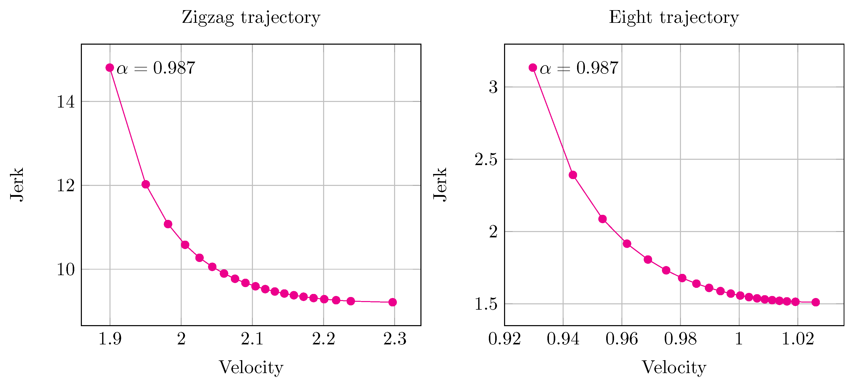
3.1. Multi-Criteria Optimization and Pareto Front

As introduced in Section 2.1, we use a composite objective (cost) function (8). This can be also solved in a series of optimizations with varying weighting factors $\alpha$, resulting in a set of optimal designs based on these weighting factor values. Each optimal design belongs to the Pareto optimal set, which is also referred to as a Pareto front. The Pareto front allows the worker or engineer to decide on the trade-off between the different objectives represented in the composite function, here smoothness and arc-length. Therefore, by exploiting this method, we avoid having to choose a value for the weighting factor $\alpha$ a priori.

The Pareto front is shown here as discretely approximated for each value of the weighting factor $\alpha$. Due to differences in magnitude between the objective functions of smoothness and arc-length, a logarithmic distribution can be chosen to ensure proper spreading of the points and, therefore, a well-approximated Pareto front. The set of constrained optimization problems leading to the Pareto front then becomes:

$$\begin{array}{cc}\hfill & \underset{\mathbf{x}}{min}\left\{F\left(\mathbf{x}\right)\right\}\hfill \\ \hfill \mathrm{where}& F={\alpha }_i{F}_1+(1-{\alpha }_i)F_2\hfill \\ \hfill & \mathbf{x}=\left[\begin{array}{cccc}{\tau }_1& {\tau }_2& \cdots & {\tau }_N\end{array}\right]\hfill \\ \hfill \mathrm{such}\mathrm{that}& \sum _i^n{\tau }_i-t_f=0\mathrm{and}{\tau }_i>0\hfill \end{array}$$

(30)

where F is the cost function in (29) and ${\tau }_i$ are the time intervals between via-points on the trajectory found via the variational problem. It should be noted that the equality constraint on time, requiring that the operation be completed in the desired amount of time, is implemented as two inequality constraints,

$$\begin{array}{cc}\hfill g_1& =\frac{{\sum }_i^N{\tau }_i}{t_f}-1\hfill \end{array}$$

(31)

$$\begin{array}{cc}\hfill g_2& =1-\frac{{\sum }_i^N{\tau }_i}{t_f}.\hfill \end{array}$$

(32)

The efficient second-order algorithm NLPQLP [30] is utilized to solve this optimization problem posed in (30)–(32). This optimization formulation, though, is general, and therefore, any gradient-based optimization algorithm can be applied.

In Section 4, it will be shown that with a relatively low number of points, the Pareto front is well defined and can be used effectively by the worker or engineer to make design decisions. It should be further pointed out that this compromise decision is to be made by a worker, and therefore, more than two or three objectives are typically not able to be handled (unable to be readily shown graphically) and therefore not advisable.

3.2. Feasibility of the Motion

Given an execution time $t_f$ fixed a priori, the trajectory resulting from an optimization from certain value $\alpha$ may result in a non-feasible trajectory. Therefore, in order to find a feasible trajectory in terms of robot limits and mechanical safety, it may have to be scaled in order to have a feasible design. However, since the arc-length does not change after a re-parametrization, we can state that for any $\alpha >0$, the solutions of (29) may be linearly scaled without losing their property of being minimum jerk trajectories.

If the planned motion violates robot limits or mechanical safety standards, we apply a linear dilation $\sigma :C^0(\mathbb{R},{\mathbb{R}}^n)⟶C^0(\mathbb{R},{\mathbb{R}}^n)$ to the computed trajectory given by:

$$\sigma \left(\mathbf{q}\left(t\right)\right)=\mathbf{q}\left({\sigma }_{0}t\right)\mathrm{with}{\sigma }_0\in {\mathbb{R}}^{+},$$

(33)

where $\sigma$ is a function that takes the continuous vector-valued trajectory $\mathbf{q}$ and returns the same trajectory scaled by the scaling factor ${\sigma }_0$.

The mechanical safety is considered by using the concept of a danger field [31], which is a map $\mathit{DF}:{\mathbb{R}}^3\times {\mathbb{R}}^n\times {\mathbb{R}}^n⟶\mathbb{R}$ such that $\mathit{DF}(\mathbf{x},\mathbf{q},\dot{\mathbf{q}})$ represents a measure of the hazard at the position $\mathbf{x}$ induced by a robot, which has its joints at positions $\mathbf{q}$ moving with speeds $\dot{\mathbf{q}}$. A robotic application is considered safe if the value of the danger field is below a given threshold ${\mathit{DF}}_{max}$ determined during the application risk assessment. In particular, we consider danger fields that are homogeneous with respect to $\dot{\mathbf{q}}$:

$$\mathit{DF}(\mathbf{x},\mathbf{q},{\sigma }_0\dot{\mathbf{q}})={\sigma }_0\mathit{DF}(\mathbf{x},\mathbf{q},\dot{\mathbf{q}}).$$

(34)

The limits of the robots are considered by taking into account the maximum values of velocity $V_{max}$ and acceleration $A_{max}$ achievable by the robot and retrieved by the data sheets and manuals provided by the robot manufacturer. If follows that, to make a motion feasible, we have to compare the given feasibility thresholds with respect to the following values:

$$\begin{array}{cc}\hfill V& =\underset{t}{max}{\parallel \dot{\mathbf{q}}\left(t\right)\parallel }_{\infty }\hfill \\ \hfill A& =\underset{t}{max}{\parallel \ddot{\mathbf{q}}\left(t\right)\parallel }_{\infty }\hfill \\ \hfill D& =\underset{t}{max}\mathit{DF}({\mathbf{x}}_0,\mathbf{q}\left(t\right),\dot{\mathbf{q}}\left(t\right)),\hfill \end{array}$$

(35)

Then, if the planned movement violates the limits of the robot or mechanical safety, the linear scaling to assure the feasibility of the motions is:

$${\sigma }_0=max\left\{\frac{V}{V_{max}},\sqrt{\frac{A}{A_{max}}},\frac{D}{D_{max}}\right\}.$$

(36)

3.3. Implemented Procedure

The final procedure implemented for running the developed methodology is as follows:

• User: definition of the trajectory via-points and desired execution time.
• Robot controller: computation of the optimal solutions and generation of the Pareto front chart.
• User: selection of the desired trajectory choosing the proper value of $\alpha$ from the Pareto front chart.
• Robot controller: Evaluation of the trajectory feasibility and, if needed, linear scaling of it.
• Robot controller: Execution of the trajectory according to the starting command given by the user.

4. Experimental Validation of the Method

4.1. Experimental Setup

The developed method and procedure was tested considering a six degree-of-freedom UR3 collaborative robot from Universal Robots available at the Smart Mini Factory laboratory of the Free University of Bozen-Bolzano [32]. The robot is an anthropomorphic robot with a non-spherical wrist, and the main characteristics are reported in Figure 1.

This robot is part of a collaborative work-cell developed by making a manual assembly operation for assembling pneumatic cylinders collaborative, as described in [33]. The operation workflow of the station consists of a pick-and-pass operation where the robot passes the required components of the assembly to the user. These components are organized a priori in a blister, and the robot trajectories are computed with our approach using the user-provided via-points. Following ISO TS-15066 [13], a mechanical risk assessment was performed [33], and the computed velocity limits are stated in

Table 1. Speed limits.

Body Region	Speed Limit (mm/s)
Upper arms and elbow joints	330
Lower arms and wrist joints	360

. In order to simplify the expression of the danger field, we suppose the source of the hazard as concentrated at the robot’s gripper. Then, the safety limits are encoded in a danger field as:

$$\mathit{DF}(\mathbf{x},\mathbf{q},\dot{\mathbf{q}})=\left\{\begin{array}{ccc}{\widehat{\mathbf{e}}}_o^{\top }\mathbf{J}\left(q\right)\dot{\mathbf{q}}\left(t\right)& \mathrm{if}& \mathbf{k}\left(\mathbf{q}\right)\in \mathcal{A}\\ 0& \mathrm{otherwise}\end{array}\right.,$$

(37)

where ${\widehat{\mathbf{e}}}_o\in {\mathbb{R}}^3$ is the direction pointing towards the operator, $\mathbf{x}$ is the Cartesian position of the gripper, $\mathbf{k}:{\mathbb{R}}^n⟶{\mathbb{R}}^3$ is the direct kinematics of the gripper, $\mathcal{A}$ is the volume of the collaborative zone, and $\mathbf{J}$ is the Jacobian matrix of the gripper’s position. In our specific case, we have ${\widehat{\mathbf{e}}}_o={[0,-1,0]}^{\top }$. To follow the trajectories, we implement a PDvelocity controller of the form:

$$\mathbf{u}={\dot{\mathbf{q}}}^{\prime }\left(t\right)+{\mathbf{K}}_p({\mathbf{q}}^{\prime }\left(t\right)-\mathbf{q}\left(t\right))+{\mathbf{K}}_d({\dot{\mathbf{q}}}^{\prime }\left(t\right)-\dot{\mathbf{q}}\left(t\right)),$$

(38)

where $\mathbf{u}$ represents the control command, ${\mathbf{q}}^{\prime }\left(t\right)$ the computed trajectory, and $(\mathbf{q}\left(t\right),\dot{\mathbf{q}}\left(t\right))$ the robot state.

4.2. Trajectories Chosen for Numerical and Experimental Comparison

In order to evaluate and validate the proposed method, two benchmark examples representing two qualitatively different motions, as well as a pick-and-pass movement for a collaborative activity have been chosen.

4.2.1. Benchmark Trajectories

The benchmark trajectories represent different shapes drawn in the horizontal plane with the end-effector; their via-points in the operational space are reported in Figure 2 and correspond to a zigzag pattern (eight via points) and to a figure-eight symbol (19 via-points), respectively. The shape of these trajectories may be appreciated in Figure 2.

The relative joint configurations, obtained via a kinematic inversion on the given path in the operational space, are reported in radians in

Table 2. Via-points for the benchmark examples.

(a) Zigzag path.
	J 1	J 2	J 3	J 4	J 5	J 6
$q_1$	−1.30	−1.94	−1.90	−0.82	1.64	−9.20
$q_2$	−1.74	−2.09	−1.66	−0.96	1.65	−9.64
$q_3$	−1.76	−1.96	−1.86	−0.89	1.65	−9.65
$q_4$	−1.26	−1.81	−2.10	−0.76	1.64	−9.15
$q_5$	−1.21	−1.66	−2.30	−0.71	1.64	−9.10
$q_6$	−1.79	−1.83	−2.04	−0.83	1.65	−9.68
$q_7$	−1.83	−1.73	−2.19	−0.80	1.65	−9.73
$q_8$	−1.16	−1.49	−2.47	−0.69	1.64	−9.05
(b) Figure-eight path.
	J 1	J 2	J 3	J 4	J 5	J 6
$q_1$	−1.16	−1.49	−2.47	−0.69	1.64	−9.05
$q_2$	−1.02	−1.57	−2.29	−0.84	1.56	−8.89
$q_3$	−1.13	−1.65	−2.21	−0.84	1.56	−9.00
$q_4$	−1.26	−1.68	−2.18	−0.84	1.56	−9.14
$q_5$	−1.35	−1.61	−2.26	−0.83	1.56	−9.23
$q_6$	−1.37	−1.50	−2.37	−0.83	1.56	−9.25
$q_7$	−1.39	−1.35	−2.49	−0.86	1.56	−9.26
$q_8$	−1.51	−1.32	−2.51	−0.87	1.55	−9.39
$q_9$	−1.66	−1.42	−2.44	−0.84	1.55	−9.54
$q_{10}$	−1.72	−1.53	−2.35	−0.82	1.55	−9.60
$q_{11}$	−1.73	−1.66	−2.22	−0.82	1.55	−9.62
$q_{12}$	−1.68	−1.74	−2.12	−0.84	1.55	−9.57
$q_{13}$	−1.61	−1.77	−2.09	−0.84	1.55	−9.50
$q_{14}$	−1.51	−1.74	−2.13	−0.84	1.55	−9.41
$q_{15}$	−1.42	−1.65	−2.25	−0.82	1.55	−9.32
$q_{16}$	−1.34	−1.50	−2.40	−0.82	1.55	−9.24
$q_{17}$	−1.23	−1.32	−2.53	−0.86	1.56	−9.14
$q_{18}$	−1.05	−1.21	−2.59	−0.91	1.56	−8.95
$q_{19}$	−0.90	−1.30	−2.54	−0.87	1.56	−8.81

.

4.2.2. Collaborative Trajectory

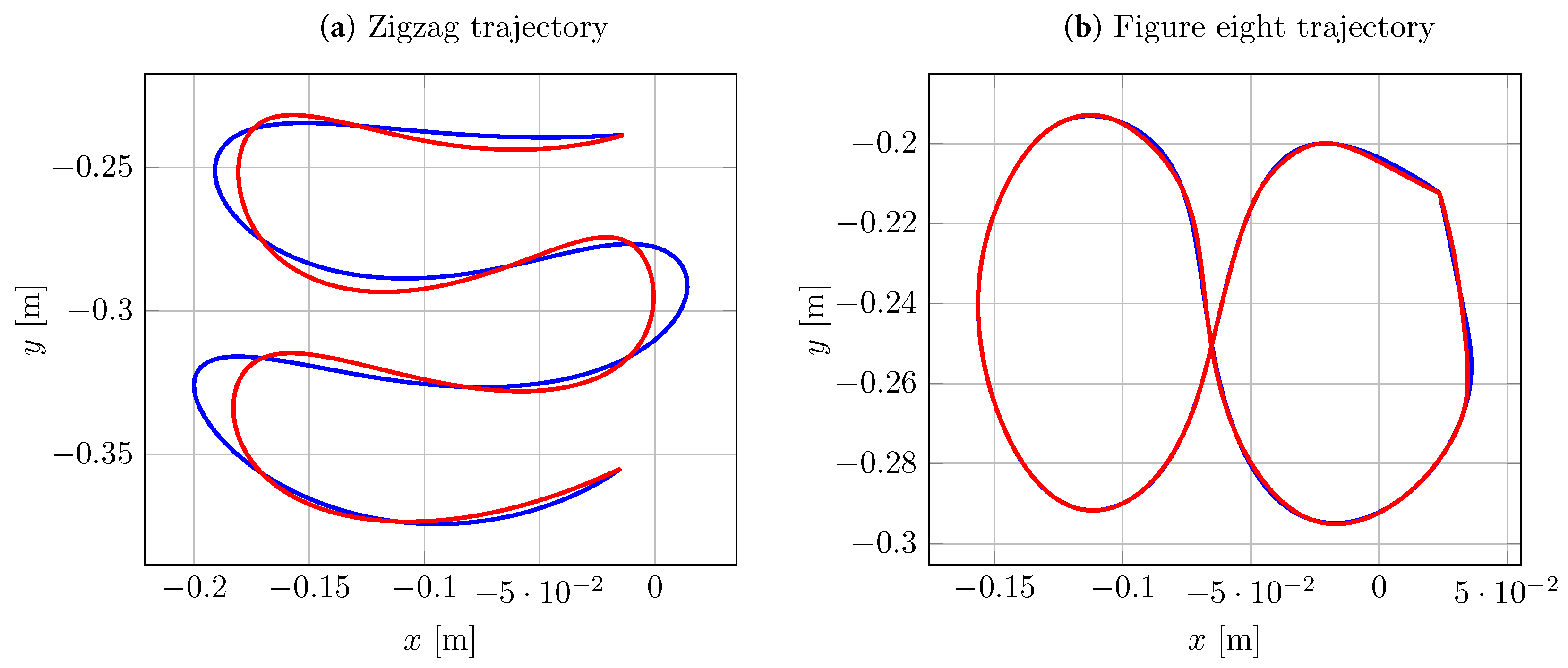
The collaborative operation consists of a pick-and-pass task composed by two consecutive movements. In the former, the robot starts from a position close to the operator and moves close to the component to be picked, approaching it for a proper grasping. Once the gripper has performed its grasping action, the latter movement is executed: the robot moves back the starting position in order to pass the object to the operator. The via-points were introduced through a hand-guiding programming phase and are reported in

Table 3. Via-points for the collaborative trajectories.

(a) Picking trajectory.
	J 1	J 2	J 3	J 4	J 5	J 6
$q_1$	−1.60	−1.90	−1.76	−2.57	−1.55	0.00
$q_2$	−0.96	−1.96	−1.76	−2.58	−1.74	0.00
$q_3$	0.78	−2.23	−1.95	−2.09	−2.36	0.00
$q_4$	0.81	−2.24	−1.93	−2.10	−2.32	0.00
$q_5$	0.87	−2.26	−1.87	−2.14	−2.27	0.00
$q_6$	0.92	−2.29	−1.80	−2.18	−2.22	0.00
(b) Passing trajectory.
	J 1	J 2	J 3	J 4	J 5	J 6
$q_1$	0.92	−2.29	−1.80	−2.18	−2.22	0.00
$q_2$	0.92	−2.23	−1.79	−2.25	−2.22	0.00
$q_3$	0.92	−2.19	−1.78	−2.30	−2.22	0.00
$q_4$	0.92	−2.15	−1.77	−2.36	−2.45	0.00
$q_5$	0.69	−2.04	−1.97	−2.26	−1.55	0.00
$q_6$	−0.77	−1.90	−1.78	−2.57	−1.55	0.00
$q_7$	−1.60	−1.90	−1.75	−2.57	−1.55	0.00

.

The required execution time given by the particular production process was 14 s.

4.3. Results

4.3.1. Benchmark Trajectories

The zigzag and figure-eight considered benchmark trajectories were evaluated for execution times of $t_f=10.5$ and $t_f=19.0$ s, respectively. Given the path and time of execution, the Pareto optimal sets were computed. Eleven discrete values of the weighting function $\alpha$ and therefore eleven separate optimizations were carried out considering the composite objective function and a logarithmic distribution used for a well-approximated Pareto front,

$$\alpha =\left\{0.999,0.998,0.996,0.992,0.984,0.968,0.937,0.874,0.749,0.499,0.001\right\}.$$

(39)

For the two sets of via-points, the optimization procedure utilized as a first guess ${\mathit{\tau }}_0=t_f/N\mathbf{1}$. To reduce computational effort, each subsequent optimization started at the previous optimum. In this study, the number of evaluations was hereby able to be reduced by approximately 30% for both cases. Further, as both sets of starting points led to the exact same results, we assumed that gradient-based optimization was effective (without commenting on the convexity of the problem). The eleven optimization runs resulting in the Pareto front for the zigzag trajectory found in Figure 3 (left) needed 98 evaluations and 72 analytical sensitivity evaluations, requiring 7.37 s on a four core Intel i5–7200U CPU with 2.50 GHz.

Physically, this solution lengthened the time on the short ends of the zigzag trajectory and shortened the time spent on the longer ends. The $L^2$ norm of the jerk was reduced, while increasing the $L^2$ norm of the velocity.

An 11 point Pareto front was also calculated for the figure-eight trajectory, and this can be seen in Figure 3 (right).Due to the higher number of via-points and therefore design variables, the complexity of the optimization was increased. Here, four-hundred thirty-eight system evaluations and 179 analytical sensitivity evaluations were required and, in turn, 65 s on the same four core Intel i5–7200U CPU with 2.50 GHz.

Being that the figure-eight path had no edges, the optimization had less effect on the arc-length and jerk values with respect to the previous benchmark trajectory. However, the jerk values can be greatly modified according to the selection of the weighting parameter.

To complement these results, in Figure 4 and Figure 5, the numerical results obtained for the two trajectories with the weighting factor $\alpha \to 0$, i.e., min-jerk trajectory in red, and with $\alpha \to 1$, i.e., arc-length minimization in red, are reported. As one might have expected, the red curve shows less overshoots with respect to the red one, in particular in the case of an “edgy” path.

4.3.2. Collaborative Trajectory

Considering the collaborative operation and the fact that it can be seen as a sequence of two movements, two Pareto fronts were computed, and the results are presented in Figure 6. The obtained trajectories (in particular, the min-jerk one) were verified taking into account the speed limits, i.e., Table 1, and a danger field (37) given by the volume with $y<-10$ cm. Thanks to these, the user can select the proper weight according to the needs and kind of movement and give to the robot controller the command for starting the execution of the chosen optimal trajectory.

To better show the developed method’s capabilities, a comparative picture was realized by computing and running three types of trajectories for the given sequence of via-points:

• a trapezoidal velocity profile generated by the robot’s controller;
• a min-jerk trajectory computed considering $\alpha \to 0$;
• a minimum arc-length trajectory computed considering $\alpha \to 1$.

A comparison of the three results is reported in Figure 7 and Figure 8 where the robot’s trapezoidal velocity profile trajectory is depicted in blue, the proposed approach is depicted with red, $\alpha \to 0$ with a dashed line and $\alpha \to 1$ with a solid line. Figure 7 shows the comparison in the joint space for the first three joints of the robot, while Figure 8 reports a comparison in the operational space in the directory of the operator (y-axis; see Figure 1). We underline that the constraints in Table 1 are respected for the given trajectories in Figure 8.

The proposed approach is inherently smoother than the robot’s trapezoidal speed profile and possibly results in being less stressful for the operator.

In

Table 4. Characteristic values.

	$max\left\{\dot{\mathit{q}}\right\}$ (rad/s)	$max\left\{\dot{\mathit{x}}\right\}$ (m/s)
Trapezoidal speed profile	1.267	0.397
$\alpha \to 0$	1.245	0.366
$\alpha \to 1$	0.844	0.245

, we present a comparison between the maximum attained velocities.

The trajectory obtained with the proposed approach with $\alpha \to 1$ showed a shorter path with respect to the one with $\alpha \to 0$ and the lowest maximum velocity. As a consequence, from the mechanical-risk point of view, the trajectory was safer with respect to the others, confirming the validity of the approach.

5. Conclusions

In this study, we address the trade-off between two constraints, namely the smoothness and speed, via a multicriteria trajectory planning approach. Smoothness is related to the cognitive stress that a person undergoes when interacting with a robot, while speed is related to safety requirements. Given an execution time, we developed the proposed method to plan safe trajectories without neglecting cognitive ergonomics and production efficiency aspects.

The balance between these two qualities was achieved through a composite objective function, and thanks to the variational formalism, a family of optimal trajectories, as well as a compact formulation for the optimization problem were presented. Thanks to the Pareto front, the operator was able to choose a trade-off between smoothness and the drawbacks of minimum jerk and obtain the trajectory that minimized the chosen cost function. Numerical and experimental results showed the feasibility of the approach, as well as the improvement of the performances both with respect to the native planner, i.e., trapezoidal speed profile, and min-jerk trajectories. Future work will cover: (i) further and extensive comparison and evaluation of the proposed method considering also the dilation effect, as well as (ii) its integration as a path option in the robot software and/or as an online service for the calculation of the optimal path and subsequent transfer to the robot.

References

1. Rojas, R.A.; Rauch, E.; Vidoni, R.; Matt, D.T. Enabling Connectivity of Cyber-Physical Production Systems: A Conceptual Framework. Procedia Manuf. 2017, 11, 822–829. [Google Scholar] [CrossRef]
2. Robots and Robotic Devices—Safety Requirements for Industrial Robots—Part 1: Robots; Standard; International Organization for Standardization: Geneva, Switzerland, 2011.
3. Robots and Robotic Devices—Safety Requirements for Industrial Robots—Part 2: Robot Systems and Integration; Standard; International Organization for Standardization: Geneva, Switzerland, 2011.
4. Robots, U. User Manual UR3/CB3 Original Instructions; Technical Report; Universal Robots: Odense, Denmark, 2017. [Google Scholar]
5. ABB. Operatingmanual IRB 14000; Technical Report; ABB: Zürich, Switzerland, 2018. [Google Scholar]
6. Gualtieri, L.; Rauch, E.; Vidoni, R.; Matt, D.T. An evaluation methodology for the conversion of manual assembly systems into human-robot collaborative workcells. Procedia Manuf. 2019, 38, 358–366. [Google Scholar] [CrossRef]
7. Gualtieri, L.; Palomba, I.; Merati, F.A.; Rauch, E.; Vidoni, R. Design of Human-Centered Collaborative Assembly Workstations for the Improvement of Operators’ Physical Ergonomics and Production Efficiency: A Case Study. Sustainability 2020, 12, 3606. [Google Scholar] [CrossRef]
8. Gualtieri, L.; Rauch, E.; Vidoni, R. Emerging Research Fields in Safety and Ergonomics in Industrial Collaborative Robotics: A Systematic Literature Review. Robot. Comput.-Integr. Manuf. 2020, 67, 101998. [Google Scholar] [CrossRef]
9. Or, C.K.; Duffy, V.G.; Cheung, C.C. Perception of safe robot idle time in virtual reality and real industrial environments. Int. J. Ind. Ergon. 2009, 39, 807–812. [Google Scholar] [CrossRef]
10. Arai, T.; Kato, R.; Fujita, M. Assessment of operator stress induced by robot collaboration in assembly. CIRP Ann. 2010, 59, 5–8. [Google Scholar] [CrossRef]
11. Lasota, P.A.; Shah, J.A. Analyzing the effects of human-aware motion planning on close-proximity human–robot collaboration. Hum. Factors 2015, 57, 21–33. [Google Scholar] [CrossRef] [PubMed] [Green Version]
12. Kokabe, M.; Shibata, S.; Yamamoto, T. Modeling of handling motion reflecting emotional state and its application to robots. In Proceedings of the SICE Annual Conference, Tokyo, Japan, 20–22 August 2008; IEEE: Piscataway, NJ, USA, 2008; pp. 495–501. [Google Scholar]
13. Robots and Robotic Devices—Collaborative Robots; Technical Specification; International Organization for Standardization: Geneva, Switzerland, 2016.
14. Gasparetto, A.; Boscariol, P.; Lanzutti, A.; Vidoni, R. Trajectory planning in robotics. Math. Comput. Sci. 2012, 6, 269–279. [Google Scholar] [CrossRef]
15. Flash, T.; Hogan, N. The coordination of arm movements: An experimentally confirmed mathematical model. J. Neurosci. 1985, 5, 1688–1703. [Google Scholar] [CrossRef] [PubMed]
16. Meirovitch, Y.; Bennequin, D.; Flash, T. Geometrical invariance and smoothness maximization for task-space movement generation. IEEE Trans. Robot. 2016, 32, 837–853. [Google Scholar] [CrossRef]
17. Oguz, O.S.; Zhou, Z.; Glasauer, S.; Wollherr, D. An Inverse Optimal Control Approach to Explain Human Arm Reaching Control Based on Multiple Internal Models. Sci. Rep. 2018, 8, 5583. [Google Scholar] [CrossRef] [PubMed]
18. Kühnlenz, B.; Kühnlenz, K. Reduction of Heart Rate by Robot Trajectory Profiles in Cooperative HRI. In Proceedings of the ISR 2016: 47st International Symposium on Robotics, Munich, Germany, 21–22 June 2016; VDE: Frankfurt, Germany, 2016; pp. 1–6. [Google Scholar]
19. Gasparetto, A.; Zanotto, V. A new method for smooth trajectory planning of robot manipulators. Mech. Mach. Theory 2007, 42, 455–471. [Google Scholar] [CrossRef]
20. Gasparetto, A.; Lanzutti, A.; Vidoni, R.; Zanotto, V. Validation of minimum time-jerk algorithms for trajectory planning of industrial robots. J. Mech. Robot. 2011, 3. [Google Scholar] [CrossRef]
21. Kyriakopoulos, K.J.; Saridis, G.N. Minimum jerk path generation. In Proceedings of the International Conference on Robotics and Automation (ICRA), Philadelphia, PA, USA, 24–29 April 1988; IEEE: Piscataway, NJ, USA, 1988; pp. 364–369. [Google Scholar]
22. Boscariol, P.; Gasparetto, A.; Vidoni, R. Planning continuous-jerk trajectories for industrial manipulators. In Engineering Systems Design and Analysis; American Society of Mechanical Engineers: New York, NY, USA, 2012; Volume 3, pp. 127–136. [Google Scholar]
23. Piazzi, A.; Visioli, A. Global minimum jerk trajectory planning of robot manipulators. IEEE Trans. Ind. Electron. 2000, 47, 140–149. [Google Scholar] [CrossRef] [Green Version]
24. Bianco, C.G.L. Minimum-jerk velocity planning for mobile robot applications. IEEE Trans. Robot. 2013, 29, 1317–1326. [Google Scholar] [CrossRef]
25. Rojas, R.A.; Garcia, M.A.R.; Wehrle, E.; Vidoni, R. A Variational Approach to Minimum-Jerk Trajectories for Psychological Safety in Collaborative Assembly Stations. IEEE Robot. Autom. Lett. 2019, 4, 823–829. [Google Scholar] [CrossRef]
26. Ehrgott, M. Multicriteria Optimization; Springer: Berlin/Heidelberg, Germany, 2005. [Google Scholar]
27. Giaquinta, M.; Hildebrandt, S. Calculus of Variations II; Springer Science & Business Media: Berlin, Germany, 2013; Volume 311. [Google Scholar]
28. Van Brunt, B. The Calculus of Variations; Universitext, Springer: New York, NY, USA, 2006. [Google Scholar]
29. Boyce, W.E.; DiPrima, R.C.; Villagómez Velázquez, H. Elementary Differential Equations and Boundary Value Problems. Ecuaciones Diferenciales y Problemas con Valores en la Frontera; Wiley: Hoboken, NJ, USA, 2004. [Google Scholar]
30. Dai, Y.H.; Schittkowski, K. A sequential quadratic programming algorithm with non-monotone line search. Pac. J. Optim. 2008, 4, 335–351. [Google Scholar]
31. Lacevic, B.; Rocco, P. Kinetostatic danger field-a novel safety assessment for human-robot interaction. In Proceedings of the International Conference on Intelligent Robots and Systems (IROS), Taipei, Taiwan, 18–22 October 2010; IEEE: Piscataway, NJ, USA, 2010; pp. 2169–2174. [Google Scholar]
32. Gualtieri, L.; Rojas, R.; Carabin, G.; Palomba, I.; Rauch, E.; Vidoni, R.; Matt, D.T. Advanced automation for SMEs in the I4. 0 revolution: Engineering education and employees training in the smart mini factory laboratory. In Proceedings of the 2018 IEEE International Conference on Industrial Engineering and Engineering Management (IEEM), Bangkok, Thailand, 16–19 December 2018; IEEE: Piscataway, NJ, USA, 2018; pp. 1111–1115. [Google Scholar]
33. Rojas, R.A.; Rauch, E.; Dallasega, P.; Matt, D.T. Safe Human-Machine Centered Design of an Assembly Station in a Learning Factory Environment. In Proceedings of the 8th International Conference on Industrial Engineering and Operations Management, Bandung, Indonesia, 6–8 March 2018. [Google Scholar]
Figure 1. UR3 robot collaborative work-cell and main data.
Applsci 10 05086 g001
Figure 2. Benchmark movements in the operational space: (a) zigzag; (b) figure-eight.
Applsci 10 05086 g002
Figure 3. Pareto fronts for the benchmark trajectories: (left) zigzag trajectory; (right) figure-eight trajectory.
Applsci 10 05086 g003
Figure 4. Numerical results for the benchmark trajectories in the operational space: (red) trajectory for α 1 and (blue) for α 0 .
Applsci 10 05086 g004
Figure 5. Numerical results for the benchmark zigzag trajectory in the joints’ space: (red) trajectory for α 1 and (blue) for α 0 .
Applsci 10 05086 g005
Figure 6. Pareto fronts for the collaborative experimental trajectories: (left) picking trajectory; (right) passing trajectory.
Applsci 10 05086 g006
Figure 7. Comparison between the different motions in the joint space. The robot’s native planner is depicted in blue; in red the proposed approach with α = 0.90 and α = 0.1 with a solid and dashed line, respectively.
Applsci 10 05086 g007
Figure 8. Comparison between the different motions of the end-effector in the direction of the operator (y-axis). The robot’s native planner is depicted in blue; in red the proposed approach with α = 0.90 and α = 0.1 with a solid and dashed line, respectively.
Applsci 10 05086 g008