Modeling, Simulation, and Vision-/MPC-Based Control of a PowerCube Serial Robot

Featured Application

The vision-based measurement of a robot’s pose investigated in this contribution is especially applicable for multi-link flexible robotic manipulators, where joint angles measured by encoders are not sufficient to describe the system’s state because of the elastic deformation of the links. The proposed MPC control scheme reveals advantages compared to common decentralized approaches concerning parameter tuning, constraint handling, and compensation of model uncertainties.

Abstract

A model predictive control (MPC) scheme for a Schunk PowerCube robot is derived in a structured step-by-step procedure. Neweul-M² provides the necessary nonlinear model in symbolical and numerical form. To handle the heavy online computational burden concerning the derived nonlinear model, a linear time-varying MPC scheme is developed based on linearizing the nonlinear system concerning the desired trajectory and the a priori known corresponding feed-forward controller. Camera-based systems allow sensing of the robot on the one hand and monitoring the environments on the other hand. Therefore, a vision-based MPC is realized to show the effects of vision-based control feedback on control performance. A semi-automatic trajectory planning is used to perform two meaningful experimental studies in which the advantages and restrictions of the proposed (vision-based) linear time-varying MPC scheme are pointed out. Everything is implemented on a slim, low-cost control system with a standard laptop PC.

1. Introduction

In contemporary robotics-research, the study of man-machine interactions is a very important area, especially in the context of robots that are released from their traditional, isolated protection cage to instead collaborate hand-in-hand with humans. For effective and efficient usage of such robots, three aspects are crucial: modeling, actuation, and sensing. Modeling plays a vital role in the development and commissioning process of such robots. Traditionally, although kinematic models for standard configurations of serial manipulators exist [1], when it comes to dynamical models these are usually derived using multibody systems (MBS) [2]. Efficient implementations for MBS already exist, providing the nonlinear equations of motion in a symbolical or numerical manner [3].

For industrial robots and modular manipulators, independent joint controllers are the most common control approach, for example, using PD or PID control schemes [4]. However, these decentralized linear control structures disregard the highly nonlinear behavior of such systems, usually do not exploit a possibly available model, fail to take information from other subsystems into account or require an elaborate tuning of the controller parameters. Another commonly used control technique, especially in trajectory tracking for rigid MBS, is the so-called computed torque method [5], which is a particular case of feedback linearization control that uses the method of inverse dynamics. Nevertheless, this model-based feed-forward control technique’s performance depends strongly on the modeling quality of the robot dynamics. Model uncertainties, that is, unmodeled, unknown or varying friction properties or a change in payload, worsen the tracking accuracy immensely. A further advanced control technique for nonlinear systems is model predictive control (MPC), also known as predictive or receding horizon control, which is firmly established in research [6] and industrial application [7]. MPC uses the advantageous capability of a model to forecast the future dynamical behavior of the system. An optimal input sequence is obtained by solving online an open-loop optimal control problem (OCP) over a finite horizon subject to system dynamics and constraints at every sample time based on the latest measurements. In case of serial manipulators, MPC offers numerous advantages, for example, handling the multivariable control problem naturally, operating as a centralized control system, intuitive adjustment of controller parameters, trajectory tracking, or considering actuator and state limitations already in the control design [8]. Thanks to the vast increase of computational power and more efficient algorithms, MPC is getting applicable to systems with fast nonlinear dynamics like a robotic system. Numerous nonlinear MPC approaches exist to reduce the computational burden of online optimization and guarantee real-time feasibility. In Reference [9], for example, a laboratory crane is controlled by a gradient-based MPC scheme using suboptimal solutions to meet the real-time requirements. In Reference [10], the control of a KUKA LWR IV robot is considered and the so-called real-time iteration scheme [11,12] solves the underlying OCP of the MPC problem, implemented in the ACADO toolkit [13]. A 6-DOF robotic arm is addressed in Reference [14], and herein the OCP is solved with the commercial interior-point-based nonlinear programming (NLP) solver FORCES PRO [15]. An approximate explicit MPC law is computed off-line beforehand for a robot manipulator in Reference [16] to bypass the online optimization, but this demands massive off-line computations and results in a static control law which loses the possibility of adapting the control law during operation to a greater extent. But all of the mentioned works use specialized and expensive hardware setups, which is in contrast to the presented and intended low-cost approach. Another popular approach to manage the contrary facts of nonlinear system behavior and expensive online calculations for solving nonlinear OCPs in real-time is first linearizing the system in some manner and then exploiting the advanced techniques developed for linear MPC. For example, for linear MPC, highly applicable real-time implementations are available as open source [17]. For this, a common approach is to use a linear time-varying (LTV) model to approximate the nonlinear system, see References [18,19,20,21]. This approach is reasonable and sufficient for the considered low-cost hardware environment because of its easy implementation in the presence of the equations of motion in a symbolic manner. Moreover, none of the mentioned MPC approaches for robotic manipulators use feedback directly obtained by a vision-based measurement of the robot’s pose to control the robot as considered in this work.

Sensing is essential for controlling the robot on the one hand and monitoring the environment on the other hand. Encoders usually provide control feedback, but camera-based systems can realize both robot state sensing and monitoring of the environment. They can detect the positions of robot links, humans, and workpieces, leading to safer and faster workflows. In this area, vision-based sensing is becoming more important, which is the second aspect of this paper. For example, it allows automatic recognition of a workpiece’s position and orientation, which therefore does not have to be positioned exactly before a robot processes it [22]. In References [23,24], stereo camera systems are used to track a flying ball and catch it with a 6-DOF robot arm. The humanoid robot Justin is even capable to catch two balls at the same time with its two arms [25,26,27]. Vision-based sensing is also an opportunity for robots with elastic links, for which the end-effector position cannot be computed from encoder signals, that is, joint angles, only.

In this paper, both MPC and a vision-based approach for gaining control feedback in real-time are combined for a serial manipulator in an experimental study. Deriving the predictive control law includes a structured step-by-step design procedure involving parameter identification and derivation of the forward and inverse dynamics. The modeling is simplified to a large extent by exploiting the advantage of having the equations of motion in a symbolical and numerical form derived by the research code Neweul-M² [3]. To handle the heavy online computational burden originating from the derived nonlinear MBS-model, a linear time-varying MPC (LTV MPC) scheme is developed based on linearizing the nonlinear system with respect to the desired trajectory and the a priori known feed-forward control torque. Instead of only using the angles measured by the built-in incremental encoders of the robot as feedback for the MPC, the robot’s current pose is detected based on images from a low-cost industrial camera as well. For this purpose, the robot is equipped with markers, which can be detected utilizing color filtering during image processing. From the detected markers’ image coordinates, the joint angles are calculated and fed back to the controller. The conducted experiments reveal the feasibility, advantages, and robustness of the proposed LTV MPC scheme when dealing with encoder feedback and show the effect of vision-based feedback on the MPC-based control loop.

Several aspects are making up the novel contributions of this work: To begin with, an encoder- and vision-based MPC is realized on a low-cost industrial-standard system, where a standard laptop PC performs the computations and process control. The controller shows that implementing and especially tuning an MPC is easy if the model equations, that is, the equations of motion, are available in symbolic form. In contrast to common control techniques, like PD or PID, adequate results are obtained with MPC without massive parameter tuning. Another novel aspect is the feedback of visually measured states, that is, joint positions, of the robot to the controller. Vision-based sensing is used in other publications as well [25,26,27], but with a different indication, that is identifying a target position for the robot’s end-effector. The actual robot movement to reach this position is then controlled based on encoder feedback, whereas in this contribution, the motion is controlled by visual feedback in real-time. In general, this contribution’s work can be seen as proof-of-concept and preparation for further studies on robots with flexible links. The position of flexible bodies cannot be described solely by encoders in the joints because of the links’ elastic deformation, whereas, for vision-based sensing, elasticity in the links can be managed. In this work, also the challenges coming along with vision-based sensing are pointed out. Moreover, the used semi-automatic trajectory planning algorithm is presented, which has been developed incidentally to avoid obstacles.

The paper is organized along with the proposed step-by-step procedure for the vision- and MPC-based control system design. Section 2 presents the available hardware, that is, the modular manipulator and camera system, as well as the lean process control system. In Section 3, the modeling is presented, including parameter identification and the derivation of the forward and inverse dynamics. Furthermore, the semi-automatic trajectory planning workflow is shown. Section 4 is dedicated to control design. A description of the image processing to measure the system states visually and runtime analysis of the vision-based control loop is found in Section 5. Section 6 presents the results of two meaningful experimental studies to point out the advantages and restrictions of the proposed LTV MPC scheme for the rigid MBS and also show the effects of vision-based control feedback on the control performance. The contribution ends with the conclusion and outlook in the final section.

2. System Setup

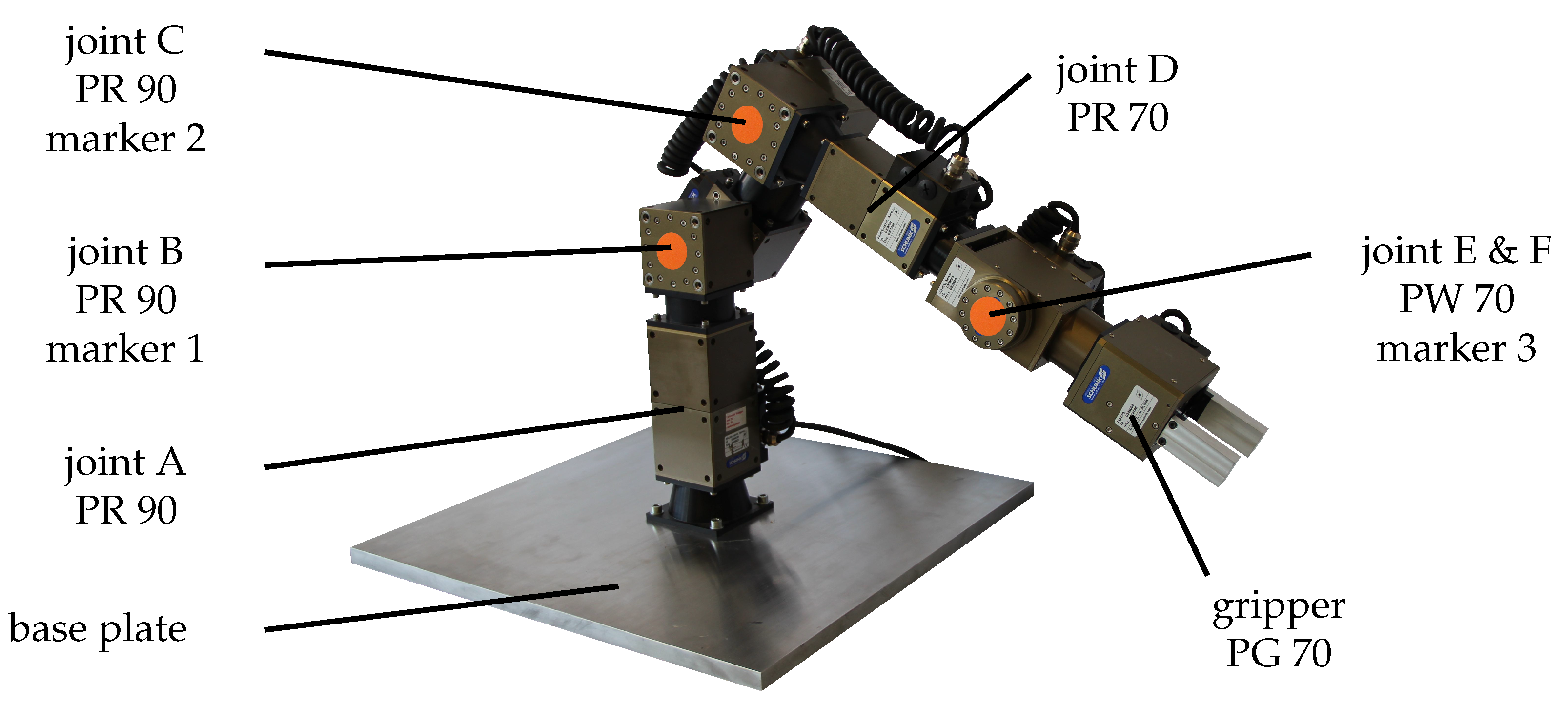
For evaluating the feasibility of the proposed MPC- and vision-based control scheme, a modular manipulator with components of the company Schunk is available, see Figure 1. Such manipulators are used for various control tasks in industrial and service robotics. The particular advantage of the concept is their modularity and their hardware’s reconfigurability. The three subsequent subsections give a short overview of the available hardware, the implemented vision-based sensing, and the lean solution of the real-time process control system.

2.1. Modular Manipulator

The serial manipulator consists of five rotary modules with six degrees of freedom (DOF) and a gripper module for carrying a load. A massive aluminum plate acts as a foundation. The first three DOF are realized by rotary units of type PR 90 (joints A, B, C) followed by the fourth DOF for which a smaller rotary unit of type PR 70 (joint D) is used. The fifth rotary unit is of type PW 70 (joint E & F) and consists of a pan-tilt unit, representing the fifth and sixth DOF. The gripper module is of type PG 70 with two prismatic fingers, and the center of the two fingers is the tool center point and end-effector position. Five connection elements link the individual units and the plate. The resulting kinematic structure of the considered configuration can be described as an anthropomorphic arm with a spherical wrist.

Table 1. Technical properties of the Schunk modules.

Module Name	Nom. Torque/Force	Max. Velocity
PR 90 (rotary) joint A & B & C	$44.8$$\mathrm{Nm}$	${\omega }_{\max }=25$$\mathrm{rpm}$
PR 70 (rotary) joint D	$10.0$$\mathrm{Nm}$	${\omega }_{\max }=25$$\mathrm{rpm}$
PW 70 (pan-tilt) joint E & F	$12.0$$\mathrm{Nm}$ & $2.0$ $\mathrm{Nm}$	${\omega }_{\max }=25$$\mathrm{rpm}$
PG 70 (gripper)	200 N	$v_{\max }=25$$\mathrm{m/s}$

lists some technical properties of the modules.

Each rotary unit has integrated control and power electronics, an incremental encoder for position and speed evaluation, and a brake for holding functions on shutdown and power failure. A brushless DC servomotor in each rotary unit directly drives a Harmonic Drive gear, which provides torque at each DOF based on the defined motor current.

For simplification, only the second and third DOF of the 6-DOF manipulator are used to validate the control scheme and all other units are positioned as depicted in Figure 1. Besides, the brakes of the unused units are applied. Consequently, this leads to a two-link manipulator with two DOF, which permits end-effector movements in a vertical plane. A two-link planar arm describes the resulting open-chain kinematic structure. For notational simplification, the rotary units B and C are denoted in the following as the first and second units, respectively.

2.2. Camera System Setup

For vision-based sensing, an IDS UI-3060CP-C-HQ Rev. 2 industrial camera is used. They can record 166 frames per second with a resolution of 2.35 megapixels ($1936\times 1216$). Further technical data include a pixel size of 5.86 μm, 11.3 mm × 7.1 mm sensor dimensions, and an optical sensor class of 1/1.2${}^{″}$. For communication with the laptop PC a USB 3.0 port is provided.

The camera’s position concerning the robot is chosen such that the image area covers all markers attached to the robot for the complete workspace of the robot. The spatial arrangement of robot and camera is shown in Figure 2, highlighted by arrows.

The image area of the camera is shown in Figure 3 for several configurations of the robot arm at the outer bounds of the workspace. As illustrated by the drawn line, the outermost marker is within the image area for the whole workspace.

The metallic surface of the foundation aluminum plate is covered by some black fabric in order to avoid light reflections that could cause problems in marker detection during image processing.

For a two-dimensional workspace of the robot, as it is the case for the experimental studies done in this paper, a single camera is sufficient for measuring the position. As soon as three-dimensional movements are allowed, a second camera for stereo vision is required.

Before the camera can be used for position estimation, the visual system has to be calibrated once utilizing a checkerboard pattern of known size. Thereby, both the internal and external camera parameters are identified, such as for example focal length and coordinate transformations.

2.3. Real-Time Process Control System

For process control, a Microsoft Windows laptop PC with Matlab R2014b and Simulink, including the additional toolboxes Real-Time Windows Target and Simulink Coder, is used. In case of vision-based control, additionally, the Image Acquisition Toolbox and the Computer Vision Toolbox are required. The laptop PC is equipped with an Intel Core i5-3210M CPU (2x2.5 GHz, 8 GB DDR3). Real-Time Windows Target [28] realizes a real-time engine for Simulink models on a Microsoft Windows PC and offers the capability to run hardware-in-the-loop simulations in real-time. It is a lean solution for rapid prototyping and provides an environment where a single computer can be used as a host and target computer. Consequently, the real-time simulations are executed in Simulink’s normal mode without an external target machine. The communication between the Simulink model running on the PC and the rotary units is implemented as follows. Schunk provides a function library written in C to communicate via a USB-CAN bus interface with the manipulator’s units. Instead of integrating the hardware via the supported input/output (I/O) boards into the loop, S-functions in the Simulink model are used for the I/O. S-functions offer the capability to integrate C code into Simulink models. For this purpose, C functions from the function library for determining the motor current, measuring the angle and angular velocity for each unit are implemented to realize I/O-communication with the rotary units.

The S-functions are compiled as MEX files using Microsoft Visual Studio C/C++ 2010 by linking the function libraries. An external power supply provides the rotary units with a constant voltage of 24 V. Because of integrated control and power electronics in each unit, no servo amplifiers are necessary. If no vision-based sensing is implemented, but encoder signals are taken as control feedback, the whole control loop and thus also the I/O-lines are processed with a sampling rate of 50 Hz, which corresponds to a sampling interval of 20 ms. The sampling rate results from the time for signal transmission via CAN bus for determining the motor current, measuring the angle and angular velocity of each unit and the calculations for the MPC. When vision-based sensing is implemented, the sampling rate is limited to 5 Hz due to the image processing algorithm’s high time requirements. For details see Section 5 and Section 6. The CAN bus works with a baud rate of 250 kBit/s.

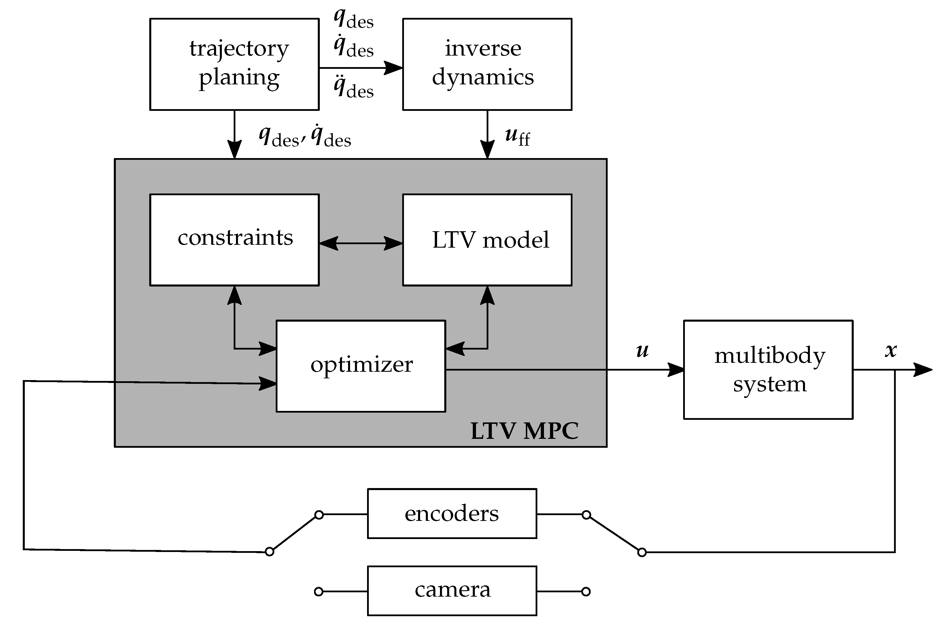
The camera is connected to the Laptop PC by a USB 3.0 connection. The Matlab Image Acquisition Toolbox offers a tool called Adaptor Kit, which is a C++ framework to create a custom adaptor, that is, a dynamic link library (DLL), for one’s own camera hardware. Having this DLL available, Matlab can communicate with the camera after loading it as a Video Input Object using the Image Acquisition Toolbox. The overall control system is visualized by Figure 4.

It is worth mentioning that the used real-time process control system is a lean and cheap solution for controlling the considered systems in real-time since no other real-time target machine or I/O boards are necessary.

3. Modeling and Trajectory Planning

The model-based MPC requires a model of the considered manipulator. As usual, in many electromechanical systems, the electrical components’ dynamics can be neglected because of much smaller time constants than the mechanical part [1]. Consequently, it is sufficient to model the dynamics of the mechanical subsystem with rigid MBS to derive the equations of motion in minimal form by describing the kinematics with generalized coordinates, see for example, Reference [2].

3.1. Forward and Inverse Dynamics

The schematic structure of the two-link manipulator and the inertial frame of reference $\{{\mathit{e}}_1,{\mathit{e}}_2,{\mathit{e}}_3\}$ used for modeling purpose are shown in Figure 5.

The links are connected by revolute joints which represent the rotary units. The considered system has $n_{\mathrm{DOF}}=2$ degrees of freedom. Consequently, the kinematics of the two-link manipulator can be described by the generalized coordinates

$$\mathit{q}={[\alpha ,\beta ]}^{\mathrm{T}},$$

(1)

defined in Figure 5. The system parameters, that is, masses $m_1$ and $m_2$, inertias $J_1$ and $J_2$, link lengths $l_0$, $l_1$ and $l_2$, and gear ratios $R_{\mathrm{PR}90}=R_1=R_2$ of the joints 1 and 2, are taken from CAD data and data sheets of the manufacturer. For the applied motor torques $T_1$ and $T_2$, a linear relation to the currents $I_1$ and $I_2$ is assumed yielding

$$T_i=R_i{k}_i{I}_i,i=1,2,$$

(2)

with the motor constants $k_i$, which have been identified manually at the hardware. Following Reference [29], the friction torque in a rotary unit PR 90 with a Harmonic Drive gear can be stated as a function of the angular velocity ${\dot{q}}_i$ in the respective unit i and the positive constants $a_j$ as

$$T_{\mathrm{fr},i}=a_1{\dot{q}}_i+a_{2}tanh\left(a_3{\dot{q}}_i\right)+a_{4}exp(-{({\dot{q}}_i/a_5)}^2)tanh\left(3a_3{\dot{q}}_i\right).$$

(3)

To avoid the discontinuous $sign$-function to describe the share of Coulomb friction, the smooth $tanh$-function, that is, the term $a_{2}tanh\left(a_3{\dot{q}}_i\right)$, is used instead. The share of viscous friction corresponds to the expression $a_1{\dot{q}}_i$ and the superelevation of the stiction of the Stribeck curve is characterized by the last summand $a_{4}exp(-{({\dot{q}}_i/a_5)}^2)tanh\left(3a_3{\dot{q}}_i\right)$.

The derivation of the equations of motion in minimal form is carried out with the Matlab-based research software Neweul-M² [3]. The forward dynamics is available for the whole six-joint PowerCube robot in Neweul-M² and therefore, the equations of motion of the whole system are available for further research. The computations are based on a Newton-Euler formalism with the application of the principle of D’Alembert [2]. Neweul-M² provides the equations of motion in a symbolical and a numerical fashion. In the latter case, Matlab’s vast numerical abilities are used to perform time integrations, kinematic analysis, and animations of the results to check the behavior of the MBS. Neweul-M² uses the Matlab Symbolic Math Toolbox for the symbolical calculations. In modeling an MBS, this offers much flexibility since the symbolic expression of the equations of motion can be edited and extended at any time. Especially in control design, it is advantageous to have the equations of motion in symbolic form to apply advanced control strategies like the proposed MPC. The systematic modeling of the considered rigid MBS leads to the nonlinear equations of motion in minimal form

$$\mathit{M}\left(\mathit{q}\right)\ddot{\mathit{q}}+\mathit{k}(\mathit{q},\dot{\mathit{q}})=\mathit{h}(\mathit{q},\dot{\mathit{q}})+\mathit{D}\mathit{u},$$

(4)

with the input vector

$$\mathit{u}={[I_1,I_2]}^{\mathrm{T}},$$

(5)

which consists of the motor currents of the first and second revolute joint, respectively. The dynamics in Equation (4) is characterized by the generalized mass matrix

$$\mathit{M}\left(\mathit{q}\right)=\left[\begin{array}{cc}{J}_1+J_2+0.25(l_1^2{m}_1+l_2^2{m}_2)+l_1^2{m}_2+l_1{l}_2{m}_{2}cos\left(\beta \right)& J_2+0.5l_2{m}_2(0.5l_2+l_{1}cos\left(\beta \right))\\ J_2+0.5l_2{m}_2(0.5l_2+l_{1}cos\left(\beta \right))& J_2+0.25l_2^2{m}_2\end{array}\right],$$

(6)

which is positive definite and symmetric, the vector of centrifugal, Coriolis and gyroscopic forces

$$\mathit{k}(\mathit{q},\dot{\mathit{q}})=\left[\begin{array}{c}-0.5{\dot{\beta }}^2{l}_1{l}_2{m}_{2}sin\left(\beta \right)-\dot{\alpha }\dot{\beta }{l}_1{l}_2{m}_{2}sin\left(\beta \right)\\ 0.5{\dot{\alpha }}^2{l}_1{l}_2{m}_{2}sin\left(\beta \right)\end{array}\right],$$

(7)

the vector of applied forces

$$\mathit{h}(\mathit{q},\dot{\mathit{q}})=\left[\begin{array}{c}0.5l_1{m}_{1}gsin\left(\alpha \right)+m_{2}gsin(\alpha +\beta )(0.5l_2+l_{1}cos\left(\beta \right))-l_1{m}_{2}gcos(\alpha +\beta )sin\left(\beta \right)-T_{\mathrm{fr},1}\\ 0.5l_2{m}_{2}gsin(\alpha +\beta )-T_{\mathrm{fr},2}\end{array}\right]$$

(8)

with the gravitational constant g, and the input matrix

$$\mathit{D}=\left[\begin{array}{cc}{R}_1{k}_1& 0\\ 0& R_2{k}_2\end{array}\right].$$

(9)

The method of inverse dynamics, or computed torque, is used to calculate a preliminary feed-forward controller for trajectory tracking. As proposed in Reference [30], this method is often most suitable for trajectory tracking of fully actuated MBS. Tracking the end-effector’s desired trajectory in the Cartesian space is achieved by successively combining inverse dynamics with an inverse kinematics scheme. For this purpose, the corresponding trajectories of the generalized coordinates are tracked, which is known in robotics as tracking in the joint space or joint trajectory tracking [1]. Therefore, the desired trajectory of the end-effector ${\mathit{r}}_{\mathrm{ee},\mathrm{des}}\left(t\right)$, ${\dot{\mathit{r}}}_{\mathrm{ee},\mathrm{des}}\left(t\right)$, and ${\ddot{\mathit{r}}}_{\mathrm{ee},\mathrm{des}}\left(t\right)$ has to be transformed from the Cartesian space into the corresponding desired trajectory of the generalized coordinates ${\mathit{q}}_{\mathrm{des}}\left(t\right)$, ${\dot{\mathit{q}}}_{\mathrm{des}}\left(t\right)$, and ${\ddot{\mathit{q}}}_{\mathrm{des}}\left(t\right)$ in the joint space. This inverse problem can be stated formally as

$${\mathit{r}}_{\mathrm{ee},\mathrm{des}}=\mathit{p}\left({\mathit{q}}_{\mathrm{des}}\right)\Rightarrow {\mathit{q}}_{\mathrm{des}}={\mathit{p}}^{-1}\left({\mathit{r}}_{\mathrm{ee},\mathrm{des}}\right),$$

(10)

where ${\mathit{p}}^{-1}:{\mathbb{R}}^3\to {\mathbb{R}}^{n_{\mathrm{DOF}}}$ is the inverse function of $\mathit{p}:{\mathbb{R}}^{n_{\mathrm{DOF}}}\to {\mathbb{R}}^3$, which describes the forward kinematics of the end-effector as a function of the generalized coordinates. For the considered case holds

$${\mathit{r}}_{\mathrm{ee}}(\alpha ,\beta )=\left[\begin{array}{c}-l_{1}sin\left(\alpha \right)-l_{2}sin(\alpha +\beta )\\ l_0+l_{1}cos\left(\alpha \right)+l_{2}cos(\alpha +\beta )\\ 0\end{array}\right].$$

(11)

The solution of the inverse problem (10) is often not unique and multiple solutions might exist. In general, the nonlinear equations of the inverse kinematics problem can be solved using numerical techniques as for instance with a Newton-Raphson method [31], by differential kinematics, or in special cases algebraically if the manipulator has a particular topology. In the case of the considered two-link manipulator (even for the available manipulator with six DOF), an algebraic closed-form solution exists, see for example Reference [32]. Neglecting the end-effector’s orientation and specifying only its position yields even in the case of a two-link planar arm two admissible postures, the so-called elbow-up and elbow-down configuration.

Substituting the desired trajectory in terms of the generalized coordinates ${\mathit{q}}_{\mathrm{des}}\left(t\right)$, ${\dot{\mathit{q}}}_{\mathrm{des}}\left(t\right)$, and ${\ddot{\mathit{q}}}_{\mathrm{des}}\left(t\right)$ into the equations of motion (4) and solving the equations for the input vector yields

$${\mathit{u}}_{\mathrm{ff}}\left(t\right)={\mathit{D}}^{-1}\left[\mathit{M}\left({\mathit{q}}_{\mathrm{des}}\left(t\right)\right){\ddot{\mathit{q}}}_{\mathrm{des}}\left(t\right)+\mathit{k}\left({\mathit{q}}_{\mathrm{des}}\left(t\right),{\dot{\mathit{q}}}_{\mathrm{des}}\left(t\right)\right)-\mathit{h}\left({\mathit{q}}_{\mathrm{des}}\left(t\right),{\dot{\mathit{q}}}_{\mathrm{des}}\left(t\right)\right)\right],$$

(12)

where ${\mathit{u}}_{\mathrm{ff}}\left(t\right)$ is the feed-forward controller. The inverse ${\mathit{D}}^{-1}$ of the input matrix always exists for a fully actuated MBS and thus the inverse model can be easily computed for a prescribed trajectory. Note that for a 3D motion, the challenge is given by describing the prescribed trajectory in the joint space considering all possible configurations, avoiding collisions and singular configurations, but this is beyond the scope of the paper. In the case of an exact model of the manipulator and no disturbances, the feed-forward controller calculated in Equation (12) would be sufficient for tracking the desired trajectory, but in a real application, the performance of the feed-forward controller depends on the quality of the derived model. Typically, the feed-forward control law (12) is used to control the MBS with an additional PD or PID feedback controller such that the decoupled dynamics of the tracking error is stable, see for example Reference [1] for details. However, in this contribution, an MPC is used to compensate model uncertainties and disturbances.

3.2. Trajectory Planning

One aim in robotics is the more straightforward commissioning of robotic systems. The robots should adapt their behavior to an unknown environment, for example, by avoiding obstacles or automatic detection and modification of end-effector target positions. Tremendous improvements were made over the last years in the robotic field. Advanced trajectory planning algorithms were developed, see for example Reference [33]. However, trajectory planning is not the main focus of this paper. Major aim of this paper is the evaluation of the MPC- and vision-based control in trajectory tracking. For a meaningful evaluation, the robot trajectory should include a motion reversal of an axis. Furthermore, due to the combination with a vision system, an integrated obstacle avoidance mechanism in trajectory planning would be an asset for further studies.

So far a simple semi-automatic procedure is developed to prepare continuous trajectories in an offline step. The workflow of trajectory planning is depicted in Figure 6. The procedure is the following:

• Based on the image of the scene, which serves as a template,
• the user specifies, that is, draws, the desired trajectory as a Bezier curve for the end-effector in Cartesian space in the program Inkscape. So far, the human user ensures an obstacle avoidance by drawing a suitable path.
• The cubic splines of the Inkscape path are then scaled and resampled within the Cartesian space in Matlab.
• From the resulting set of end-effector points along the trajectory L sample points are chosen.
• Afterwards, feasible joint coordinates are calculated for each of the L sample points with the help of inverse kinematics, see Equation (10), and the Neweul-M² model of the robot, and the desired velocity at the intermediate points is specified.
• For every joint those calculated joint coordinates are then combined into a continuous motion via a spline as described in Reference [34]. Instead of using a single polynomial of degree $L-1$ for interpolation, which often leads to oscillations, $L-1$ cubic polynomials are used to interpolate the trajectory parts. As stated above, the resulting function is a spline with minimal curvature. The degree of those polynomials is chosen to three to guarantee continuity of the resulting velocity and acceleration profile. In between those calculations an optimization process minimizes the overall time T needed for the trajectory subject to not exceeding maximum joint velocities ${\dot{q}}_{i,\max }$ and accelerations ${\ddot{q}}_{i,\max }$ for each joint i. At first, the time each of the joints needs for the trajectory is minimized by computing the intermediate times $T_{k,i}$ for each joint i and polynomial segment $k=1,\cdots ,L-1$. Afterwards, the maximum of the times $T_{k,i}$ needed by each individual joint is taken as the resulting intermediate time for all joints, that is,

  $$\begin{array}{ccc}{T}_k\hfill & =\hfill & \underset{i}{\max }{T}_{k,i}\hfill \\ \hfill & \hfill & \mathrm{s}.\mathrm{t}.|{\dot{q}}_i|\le {\dot{q}}_{i,\max }\hfill \\ \hfill & \hfill & |{\ddot{q}}_i|\le {\ddot{q}}_{i,\max }\hfill \end{array}\mathrm{and}T=\sum _k{T}_k.$$

  (13)
• The resampled results, containing joint positions, velocities, and accelerations as well as a time vector, are then simulated, animated, and checked for collisions in order to see offline if, for example, the joint restrictions are kept. Rank deficiencies in the Jacobian matrix $\mathit{J}\left(\mathit{q}\right)=\partial {\mathit{r}}_{\mathrm{ee}}\left(\mathit{q}\right)\partial /\mathit{q}$, provided from Neweul-M² in a symbolical fashion, indicate singular configurations. Those singularities should be avoided in the trajectory. Finally, the trajectory can be processed on the actual robot.

4. Control Design

The advanced control methodology MPC is based on a receding horizon strategy in which the control input is calculated by solving repetitive optimal control problems (OCP) over a finite time horizon taking the system dynamics and possible constraints for states and inputs directly into account. When dealing with highly nonlinear system dynamics as in the considered case, a nonlinear MPC strategy is necessary which, in general, suffers from the need of solving efficiently a nonlinear optimization problem at each time step in real-time. In the presence of an adequate feed-forward controller, the computational burden can be circumvented by using a linear time-varying (LTV) model approximation of the nonlinear system dynamics with respect to the desired trajectory and feed-forward control signal. Then, a so-called LTV MPC can be designed and only a linear-quadratic optimization problem has to be solved at each time step.

4.1. Linear Time-Varying Model Approximation

At first, the second order differential equation of motion (4) is transformed into a first order system yielding

$$\begin{array}{c}\hfill \dot{\mathit{x}}=\mathit{f}(\mathit{x},\mathit{u})=\left[\begin{array}{c}\dot{q}\\ {\mathit{M}}^{-1}\left(\mathit{q}\right)\left(\mathit{h}(\mathit{q},\dot{\mathit{q}})-\mathit{k}(\mathit{q},\dot{\mathit{q}})\right)\end{array}\right]+\left[\begin{array}{c}\mathbf{0}\\ {\mathit{M}}^{-1}\left(\mathit{q}\right)\mathit{D}\end{array}\right]\mathit{u},\end{array}$$

(14)

where the state vector $\mathit{x}={\left[{\mathit{q}}^{\mathrm{T}},{\dot{\mathit{q}}}^{\mathrm{T}}\right]}^{\mathrm{T}}\in {\mathbb{R}}^n$ consists of the generalized coordinates q and velocities $\dot{\mathit{q}}$ with $n=2n_{\mathrm{DOF}}$. The function $\mathit{f}:{\mathbb{R}}^n\times {\mathbb{R}}^m\to {\mathbb{R}}^n$ describes the system dynamics as a function of the states x and inputs $\mathit{u}\in {\mathbb{R}}^m$. With regard to safety requirements of the motor currents or mechanical limitations like limited space or velocities, system (14) is subject to state and input constraints stated as

$$\mathit{x}\left(t\right)\in \mathcal{X},\mathit{u}\left(t\right)\in \mathcal{U},$$

(15)

where $\mathcal{X}\subseteq {\mathbb{R}}^n$ and $\mathcal{U}\subseteq {\mathbb{R}}^m$ are polytopes. In case of simple limitations, the sets $\mathcal{X}$ and $\mathcal{U}$ are given by box constraints of the form

$$\mathcal{X}=\{x\in {\mathbb{R}}^n\mid x_{\min }\le x\le x_{\max }\}\mathrm{and}\mathcal{U}=\{x\in {\mathbb{R}}^m\mid u_{\min }\le u\le u_{\max }\}.$$

(16)

Assuming that the actual state and input of the system is in a neighborhood of the desired trajectory and feed-forward controller, the nonlinear system (14) can be linearized with respect to the desired trajectory ${\mathit{x}}_{\mathrm{des}}\left(t\right)={\left[{\mathit{q}}_{\mathrm{des}}{\left(t\right)}^{\mathrm{T}},{\dot{\mathit{q}}}_{\mathrm{des}}{\left(t\right)}^{\mathrm{T}}\right]}^{\mathrm{T}}$ and the feed-forward controller ${\mathit{u}}_{\mathrm{ff}}\left(t\right)$ from Equation (12) resulting in the LTV system

$$\Delta \dot{\mathit{x}}\left(t\right)=\mathit{A}\left(t\right)\Delta \mathit{x}\left(t\right)+\mathit{B}\left(t\right)\Delta \mathit{u}\left(t\right),$$

(17)

where the time-varying system matrices $\mathit{A}\left(t\right)\in {\mathbb{R}}^{n\times n}$, $\mathit{B}\left(t\right)\in {\mathbb{R}}^{n\times m}$ and the deviations $\Delta \mathit{x}\left(t\right)$, $\Delta \mathit{u}\left(t\right)$ are given as

$$\mathit{A}\left(t\right)={\displaystyle \frac{\partial \mathit{f}}{\partial \mathit{x}}}{|}_{{\mathit{x}}_{\mathrm{des}}\left(t\right),{\mathit{u}}_{\mathrm{ff}}\left(t\right)}\prime \mathit{B}\left(t\right)={\displaystyle \frac{\partial \mathit{f}}{\partial \mathit{u}}}{|}_{{\mathit{x}}_{\mathrm{des}}\left(t\right),{\mathit{u}}_{\mathrm{ff}}\left(t\right)}\prime$$

(18)

$$\Delta \mathit{x}\left(t\right)=\mathit{x}\left(t\right)-{\mathit{x}}_{\mathrm{des}}\left(t\right),\Delta \mathit{u}\left(t\right)=\mathit{u}\left(t\right)-u_{\mathrm{ff}}\left(t\right).$$

(19)

The continuous LTV system (17) describes the dynamics of the deviations of the nonlinear system (14) from the desired trajectory ${\mathit{x}}_{\mathrm{des}}\left(t\right)$ and feed-forward controller ${\mathit{u}}_{\mathrm{ff}}\left(t\right)$. Note that in the presence of the equations of motion in symbolical form, the previous calculations can be done easily by the Matlab Symbolic Math Toolbox.

Implementing a controller on a digital control unit leads indispensably to discretization. Consequently, the desired trajectory and the feed-forward controller have to be sampled and the continuous LTV system (17) has to be discretized subject to the sampling interval $\Delta T$ of the real-time process control system. Therefore, consider the time discretization $t_k=k\Delta T$ with sampling instance $k=0,1,2,\cdots ,t_{\mathrm{f}}/\Delta T$. For notational simplification, let $\Delta \mathit{x}\left(k\right)=\Delta \mathit{x}\left(t_k\right)$, $\Delta \mathit{u}\left(k\right)=\Delta \mathit{u}\left(t_k\right)$, and so on. By assuming zero-order hold for the inputs $\Delta \mathit{u}\left(t\right)$ over the sampling interval $t\in \left[t_k,t_{k+1}\right)$, the continuous LTV system (17) can be discretized into a linear discrete time-varying system

$$\Delta \mathit{x}(k+1)={\mathit{A}}_{\mathrm{d}}\left(k\right)\Delta \mathit{x}\left(k\right)+{\mathit{B}}_{\mathrm{d}}\left(k\right)\Delta \mathit{u}\left(k\right),$$

(20)

with

$${\mathit{A}}_{\mathrm{d}}\left(k\right)=exp\left(\mathit{A}\left(k\right)\Delta T\right),{\mathit{B}}_{\mathrm{d}}\left(k\right)=\left({\int }_0^{\Delta T}exp\left(\mathit{A}\left(k\right)\tau \right)\mathrm{d}\tau \right)\mathit{B}\left(k\right).$$

(21)

Hence, the nonlinear system (14) is discretized and linearized concerning several operating points $\left({\mathit{x}}_{\mathrm{des}}\left(k\right),{\mathit{u}}_{\mathrm{ff}}\left(k\right)\right)$, which result from the sampled desired trajectory and feed-forward controller.

4.2. Linear Time-Varying Model Predictive Control

Based on these preliminary calculations, the following OCP can be stated at each sampling time $t_k$ or sampling instance k, respectively, as

$$\begin{array}{cc}& \underset{\Delta \bar{\mathit{u}}\left(k\right),\cdots ,\Delta \bar{\mathit{u}}(k+N-1)}{\min }\left\{\sum _{l=k}^{k+N-1}{∥\Delta \bar{x}\left(l\right)-\Delta x_{\mathrm{des}}\left(l\right)∥}_{\mathit{Q}}^2+{∥\Delta \bar{u}\left(l\right)-\Delta \bar{u}(l-1)∥}_{\mathit{R}}^2\right\},\hfill \end{array}$$

(22)

$$\begin{array}{cc}\hfill \mathrm{s}.\mathrm{t}.& \Delta \bar{\mathit{x}}(l+1)={\mathit{A}}_{\mathrm{d}}\left(k\right)\Delta \bar{\mathit{x}}\left(l\right)+{\mathit{B}}_{\mathrm{d}}\left(k\right)\Delta \bar{\mathit{u}}\left(l\right),\hfill \end{array}$$

(23)

$$\begin{array}{cc}& \Delta \bar{\mathit{x}}\left(k\right)=\mathit{x}\left(k\right)-{\mathit{x}}_{\mathrm{des}}\left(k\right),\hfill \end{array}$$

(24)

$$\begin{array}{cc}& \Delta \bar{\mathit{u}}(k-1)=\mathit{u}(k-1)-{\mathit{u}}_{\mathrm{ff}}\left(k\right),\hfill \end{array}$$

(25)

$$\begin{array}{cc}& \Delta \bar{\mathit{x}}\left(l\right)\in \mathcal{X}\left(k\right)=\left\{\Delta \bar{\mathit{x}}\in {\mathbb{R}}^n\mid {\mathit{x}}_{\min }-{\mathit{x}}_{\mathrm{des}}\left(k\right)\le \Delta \bar{\mathit{x}}\le {\mathit{x}}_{\max }-{\mathit{x}}_{\mathrm{des}}\left(k\right)\right\},\hfill \end{array}$$

(26)

$$\begin{array}{cc}& \Delta \bar{\mathit{u}}\left(l\right)\in \mathcal{U}\left(k\right)=\left\{\Delta \bar{\mathit{u}}\in {\mathbb{R}}^m\mid {\mathit{u}}_{\min }-{\mathit{u}}_{\mathrm{ff}}\left(k\right)\le \Delta \bar{\mathit{u}}\le {\mathit{u}}_{\max }-{\mathit{u}}_{\mathrm{ff}}\left(k\right)\right\},\hfill \\ & l=k,k+1,\cdots ,k+N-1\hfill \end{array}$$

(27)

by introducing $\Delta {\mathit{x}}_{\mathrm{des}}\left(l\right)={\mathit{x}}_{\mathrm{des}}\left(l\right)-{\mathit{x}}_{\mathrm{des}}\left(k\right)$, which denotes the deviation of the desired trajectory to the current operating point. The box constraints concerning the current operating point, that is, Equations (26) and (27), are stated in a similar manner. Note that the predicted states and inputs in the OCP are equipped with an additional bar, since the predicted trajectories do not coincide with the actual closed-loop trajectories, even for no plant-model mismatch because of the finite prediction horizon N, see for example Reference [35] for details. The OCP is initialized by the measured state $\mathit{x}\left(k\right)$ and the previously implemented input $\mathit{u}(k-1)$. As usual in linear MPC, a quadratic cost function (22) is considered using standard MPC notation, where $\mathit{Q}\in {\mathbb{R}}^{n\times n}$ and $\mathit{R}\in {\mathbb{R}}^{m\times m}$ are positive definite weighting matrices of appropriate dimensions. The first summand in Equation (22) represents the penalty on tracking errors subject to the desired trajectory, and the second summand penalizes changes in the input vector. Hence, it is necessary to include the previous input into the OCP. Penalizing changes in the input vector offers the capability to weight the aggressiveness of the controller and to suppress oscillating input trajectories such to prevent oscillations of the system. The weighting matrices Q and R as well as the prediction horizon N are the tuneable parameters to obtain a required performance of the controller. The optimization at each time step is subject to the LTV system dynamics (23) concerning the fixed operation point $\left({\mathit{x}}_{\mathrm{des}}\left(k\right),{\mathit{u}}_{\mathrm{ff}}\left(k\right)\right)$ at the respective time instance k. To reduce the computational complexity of the LTV MPC scheme, the changes of operating points are not considered in the prediction as it is also assumed for application in Reference [18]. In terms of small prediction horizons this approximation is appropriate.

To solve the OCP from Equations (22)–(27) at each sampling instance k, it is convenient to condense the problem by introducing the optimization vector

$$\Delta \bar{\mathit{w}}\left(k\right)=\left[\begin{array}{c}\Delta \bar{\mathit{z}}\left(k\right)\\ \Delta \bar{\mathit{z}}(k+1)\\ ⋮\\ \Delta \bar{\mathit{z}}(k+N-1)\end{array}\right]=\left[\begin{array}{c}\Delta \bar{\mathit{u}}\left(k\right)-\Delta \mathit{u}(k-1)\\ \Delta \bar{\mathit{u}}(k+1)-\Delta \bar{\mathit{u}}\left(k\right)\\ ⋮\\ \Delta \bar{\mathit{u}}(k+N-1)-\Delta \bar{\mathit{u}}(k+N-2)\end{array}\right].$$

(28)

Then as usual in linear MPC, the OCP from Equations (22)–(27) can be transformed into a linear-quadratic optimization problem

$$\begin{array}{cc}\hfill \underset{\Delta \overline{\mathit{w}}\left(k\right)}{\min }& \left\{\frac{1}{2}\Delta \overline{\mathit{w}}{\left(k\right)}^{\mathrm{T}}\mathit{H}\left(k\right)\Delta \overline{\mathit{w}}\left(k\right)+\Delta \overline{\mathit{w}}{\left(k\right)}^{\mathrm{T}}\mathit{d}\left(k\right)\right\},\hfill \end{array}$$

(29)

$$\begin{array}{cc}\hfill \mathrm{s}.\mathrm{t}.& \mathit{F}\left(k\right)\Delta \overline{\mathit{w}}\left(k\right)\le \mathit{v}\left(k\right),\hfill \end{array}$$

(30)

see for example Reference [8] for details and for derivation of the matrices $\mathit{H}\left(k\right)\in {\mathbb{R}}^{N\times N}$, $\mathit{F}\left(k\right)\in {\mathbb{R}}^{p\times N}$, and the vectors $\mathit{d}\left(k\right)\in {\mathbb{R}}^N$, $\mathit{v}\left(k\right)\in {\mathbb{R}}^p$, where p is the number of constraints following from Equations (26) and (27). Denoting the optimal solution of Equations (29) and (30) by $\Delta {\bar{\mathit{w}}}^{*}\left(k\right)$, the implemented control input $\mathit{u}\left(k\right)$ on the plant follows from

$$\mathit{u}\left(k\right)\stackrel{\left(19\right)}{=}{\mathit{u}}_{\mathrm{ff}}\left(k\right)+\Delta {\bar{\mathit{u}}}^{*}\left(k\right)\stackrel{\left(28\right)}{=}{\mathit{u}}_{\mathrm{ff}}\left(k\right)+\Delta (k-1)+\Delta {\bar{\mathit{z}}}^{*}\left(k\right)$$

(31)

with $\Delta \mathit{u}(k-1)$ from Equation (25). Note that only the first piece of the optimal input trajectory is applied whereas the remaining part is discarded. The presented LTV MPC scheme is summarized by Algorithm 1.

Algorithm 1: LTV MPC scheme

1: obtain state measurements $\mathit{x}\left(k\right)$ either from encoders or camera 2: prepare matrices $\mathit{H}\left(k\right)$, $\mathit{F}\left(k\right)$, and the vectors $\mathit{d}\left(k\right)$, $\mathit{v}\left(k\right)$ for the linear-quadratic optimization problem from Equations (29) and (30) at the current sampling instance k and the current operating point $\left({\mathit{x}}_{\mathrm{des}}\left(k\right),{\mathit{u}}_{\mathrm{ff}}\mathit{x}\left(k\right)\right)$ based on the measurement $\mathit{x}\left(k\right)$, the previous input $\mathit{u}(k-1)$, the linearized system (23), the desired trajectory ${\mathit{x}}_{\mathrm{des}}\left(k\right)$, the state (26), and input constraints (27) 3: compute the optimal input vector $\Delta {\bar{\mathit{w}}}^{*}\left(k\right)$ by solving the linear-quadratic optimization problem from Equations (29) and (30) 4: implement $\mathit{u}\left(k\right)$ due to Equation (31) to the plant 5: shift the prediction horizon and operating point by one time step and continue with step 1

By linearizing the nonlinear system (14) around the a priori known desired trajectory and feed-forward controller, several computations of step 2 can be done offline leading to a reduced calculation time and an advantage of the presented LTV MPC scheme over the corresponding complete online approach. Figure 7 shows and summarizes the generalized topology of the closed control loop.

It is remarked that the proposed LTV MPC scheme does not necessarily guarantee stability of the closed control loop, which follows directly from considering a finite prediction horizon, see Reference [35]. In the literature, see for example Reference [36], stability is usually achieved by introducing terminal costs and terminal inequality constraints. Moreover, for LTV MPC the interested reader can find a formal stability proof in Reference [19] under some reasonable assumptions. However, for applicability, the feasibility of the OCP, and real-time capability, in this conceptual investigation stability is achieved by choosing the prediction horizon sufficiently long as usual in MPC application.

5. Vision-Based Sensing

Instead of using the signals from the robot’s incremental encoders as control feedback, the joint angles can also be determined by evaluating images from a camera system. The necessary experimental setup and the implemented image processing are in the scope of this section.

5.1. Marker Detection

In order to measure the current robot position visually, circular-shaped orange markers with a diameter of 4 cm are attached to three decisive points on the robot, see Figure 1. The marker detection can be realized based on different criteria. The first option is a color-based detection, where the desired objects are identified with the help of color filters [23,24]. The second option is a shape-based detection, that is, to identify circles in the image. For this, a variant of the Hough transform or a Sobel filter can be used as in Reference [27]. Another option would be the comparison of the current image with a reference image [37]. By computing the difference of both images, moving objects can be detected.

The latter method based on image differences is not suitable here, since not only the three markers but all the moving parts of the robot would be detected. For a shape-based marker detection, first edges have to be detected, for example by means of the Canny algorithm [38], before the circles can be identified using the Hough transform [39]. Since this process takes about two seconds, the markers are tracked, for example, with the Kanadi-Lucas-Tomasi method (KLT tracking) [40,41] after they have been identified once. Unfortunately, often points get lost after a few seconds, as experiments show, and the markers have to be identified once again, which takes too long for real-time execution. Therefore, the shape-based detection method is unsuitable here as well.

The detection method chosen for the application presented in this paper is color-based. The images are analyzed in HSV color space, which is short for hue, saturation, and value. Hue stands for the color, for example, red, green, or blue, saturation indicates the colorfulness, and value corresponds to the brightness. The HSV color space is particularly suitable, since different shades are to be found coherently in one sector of the color space and can therefore be described independently from the brightness. The brightness of the ambient light thus has only little influence on the result.

The individual steps of the color filtering process are visualized in Figure 8.

The filter parameters have to be adjusted such that the areas of the original image, see Figure 8a, which contain a marker, pass the filter completely, while the environment is filtered out as accurately as possible. Thereby, a binary image, see Figure 8b, is created, which still contains some artifacts though, that is, pixels of the environment that passed the filter erroneously. To get rid of those, the morphological operation called opening is applied [42], yielding the image in Figure 8c, which contains exactly the desired markers. The center points of the remaining areas are the marker coordinates.

One-time at the beginning, the identified image coordinates have to be assigned to the corresponding markers. Afterwards, the matching can be done automatically using shortest distances to marker positions from the preceding image.

The main advantage of this method is on the one hand the significantly lower computation time compared to shape-based detection by Hough transform. On the other hand, it is still slower than KLT tracking. However, in total the advantages of color-based detection prevail. It allows a reliable detection of the markers during the complete period of robot movement with a time step size still suitable for real-time application.

5.2. Coordinate Transformation

From the identified image coordinates of the markers the joint angles, that is, the generalized coordinates, have to be computed in a second step. To do so, lens distortions, which make straight lines in real world look curved in the image, have to be eliminated first. For this purpose, the Matlab function undistortPoints from the Computer Vision Toolbox is available. Then, with the Matlab function pointsToWorld, the x- and y-coordinates of the markers given in the checkerboard coordinate system from calibration are obtained. Coordinate transformation to the desired world coordinate system is then realized by simple translation and rotation. Taking the offsets between the markers on the robot’s surface and the joint center points into account, the center point coordinates $[x_1,y_1]$, $[x_2,y_2]$, $[x_3,y_3]$ of the joints equipped with markers are obtained in the world coordinate system. The joint angles $\alpha$ and $\beta$, see Figure 5, are finally computed by the trigonometric relations

$$\begin{array}{ccc}\hfill \alpha & =& \mathrm{atan}2(x_2-x_1,y_2-y_1),\hfill \end{array}$$

(32a)

$$\begin{array}{ccc}\hfill \beta & =& \alpha -\mathrm{atan}2(x_3-x_2,y_3-y_2),\hfill \end{array}$$

(32b)

where atan2 is the four-quadrant inverse tangent function. The indices represent the numbers of the markers according to Figure 1.

Note that for tracking a spatial movement with more than two degrees of freedom, at least a second camera is necessary to set up a stereo vision system. Then, the transformation of marker coordinates from an image coordinate system to the checkerboard coordinate system or world coordinate system, respectively, is done by triangulation. In case of 3D motion, there is a risk for markers to be hidden behind the robot’s parts depending on its configuration and the camera positions. Therefore, these markers would be invisible for one or more cameras making a localization of the respective robot parts impossible. To address this problem, more cameras and/or markers are required to capture the mechanical components’ position for the complete workspace and all possible robot configurations. To do so, a motion capture system like OptiTrack might be used as it is done in Reference [43] to capture human motion in a driver-in-the-loop simulator or in Reference [44] to capture the motion of a flying robot. However, using a motion capture system contradicts the low-cost approach of slim hardware requirements pursued in this contribution.

5.3. Real-Time Capability

To use visual feedback from a single camera instead of incremental encoder signals, a time step size of 200 ms is required for real-time execution of the closed control loop. This is ten times as much as the time step size of 20 ms that is sufficient when encoder signals are used. Therefore, runtime is analyzed and time requirements of the individual control loop components are visualized in Figure 9.

The inner circle ring represents the top level, while the middle and outer circle rings give a more detailed view of single subsystems.

On average, the entire computation takes 127 ms per sampling instance. Thereof, 10 ms are claimed by the camera for image acquisition and 14 ms for communication with the robot. The major portion of 80 %, which corresponds to 102 ms, is taken by the image processing part. A more detailed investigation of the image processing, shown in the middle ring, reveals that most of the time is required to detect the markers in the image. Breaking down things on an even lower level shows in the outer ring that color filtering is the most time-consuming part, taking 57 ms. This makes up for almost half of the time required for the overall control loop.

The reason for the high time requirements of color filtering and image processing in general is the big amount of data that needs to be processed. During the filtering process, about ten comparison operations, for example with color threshold values, have to be executed for each pixel. Even with a subsampled image resolution of $968\times 608\approx$ 600,000 pixels the required computation time is accordingly high.

6. Experimental Studies

The proposed LTV MPC scheme described in Section 4 is applied to the two-link manipulator in two ways. In the first study, the performance and robustness of the implemented LTV MPC scheme is demonstrated. For this purpose, the state measurement is obtained directly from the encoders and allows a sampling interval of 20 ms. In order to demonstrate the performance with vision-based state measurement, the control loop is closed with visual feedback instead of encoders in the second scenario. This requires a sampling interval of 200 ms, which results in limited performance of the overall closed-loop system.

In both studies, the MPC cost function (22) is parameterized by diagonal weighting matrices to penalize the control error with respect to the desired trajectory, that is, $\mathit{Q}=\mathrm{diag}\left([Q_{\alpha },Q_{\beta },Q_{\dot{\alpha }},Q_{\dot{\beta }}]\right)=\mathrm{diag}\left([100,100,0.1,0.1]\right)$, whereas the changes in the input are weighted by $\mathit{R}=\mathrm{diag}\left([R_{\Delta I_1},R_{\Delta I_2}]\right)=\mathrm{diag}\left([1,1]\right)$. A preliminary adjustment of the parameters has been obtained by simulations followed by re-adjusting the weights at the hardware. In order to not exceed the maximum currents of the rotatory modules, the constraints for the inputs are determined by $I_{1,\min }=I_{2,\min }=-4\mathrm{A}$ and $I_{1,\max }=I_{2,\max }=4\mathrm{A}$. Moreover, a prediction horizon of $N=5$ is chosen and the controller is initialized by $\mathit{x}\left(0\right)={\mathit{u}}_{\mathrm{des}}\left(0\right)$ and $\mathit{u}(-1)={\mathit{u}}_{\mathrm{ff}}\left(0\right)$. The repetitive linear-quadratic optimization problem from Equations (29) and (30) is solved by using the active set method applying the open-source implementation qpOASES [17].

For interpreting the results, it is mentioned that the encoders can measure the angular velocity of the modules with a resolution of 0.04 rad/s = 2.29 deg/s.

6.1. Encoder-Based Tracking

In the first scenario, the performance of the LTV MPC scheme is evaluated using feedback from the encoders. The considered trajectory of the end-effector is designed as described in Section 3.2 and the path is illustrated in Figure 10, whereas the complete motion of the manipulator can be seen in the deposited video (https://www.itm.uni-stuttgart.de/en/research/vision-based-control-of-a-powercube-robot/).

Note that the trajectory is motivated by an obstacle avoidance and includes motion reversals in both joints to investigate the control performance on friction phenomena caused by the Harmonic Drive gears that underly highly nonlinear friction effects.

Figure 11 illustrates experimental results of the considered motion.

Therefore, the measured values of generalized coordinates and velocities are compared with the desired trajectories. In addition, the applied motor currents determined by the MPC, that is, $I_{1,\mathrm{appl}}$ and $I_{2,\mathrm{appl}}$, are compared with the preliminarily calculated feed-forward controller based on Equation (12). For validation purpose, the control error of the end-effector is defined as

$$e_{\mathrm{ee},\mathrm{enc}}=\parallel {\mathit{r}}_{\mathrm{ee},\mathrm{enc}}-{\mathit{r}}_{\mathrm{ee},\mathrm{des}}\parallel$$

(33)

and shown in Figure 12. Thereby, ${\mathit{r}}_{\mathrm{ee},\mathrm{enc}}={\mathit{r}}_{\mathrm{ee}}({\alpha }_{\mathrm{enc}},{\beta }_{\mathrm{enc}})$ and ${\mathit{r}}_{\mathrm{ee},\mathrm{des}}={\mathit{r}}_{\mathrm{ee}}({\alpha }_{\mathrm{des}},{\beta }_{\mathrm{des}})$ are the end-effector positions computed by the forward kinematics with the generalized coordinates measured by the encoders or with the desired generalized coordinates, respectively.

Obviously, the proposed LTV MPC scheme works well and can track the predefined trajectory with high accuracy in terms of the angle and angular velocities. Moreover, the proposed control structure can easily handle the predefined input constraints, which can be seen during the period $6.0\mathrm{s}\le t\le 7.5\mathrm{s}$ as the second joint reaches its input constraints whereby the motor in fact has to provide higher torques to track the desired trajectory. As a result, the tracking error of the end-effector increases, see Figure 12. In contrast to a PID controller, no wind-up effects occur, no additional anti-wind-up control structure is necessary to handle input constraints, and due to the centralized control structure all states are taken into account to compute the inputs to reduce the control error in an optimal manner. The controller also deals with reversing motor directions and treats the occurring friction phenomena, which occur at sign changes in the velocities. Nevertheless, by comparing the implemented and the feed-forward motor currents, it becomes clear that there is a notable deviation. This deviation originates from uncertainties and disturbances since in the case of a perfect model and no disturbances the feed-forward controller (12) would be sufficient. Despite the distinct model uncertainties, the proposed LTV MPC scheme compensates these uncertainties well and thus reveals its robustness. Consequently, the modeling and parameter identification efforts can be extremely reduced with the proposed LTV MPC scheme compared to a pure feed-forward controller. Furthermore, the command response, as well as changes in the input, can easily be adjusted and weighted by a modification of the weighting parameters for the states or inputs in the cost functional, which is much more intuitive and evident than tuning the parameters of a classical PD or PID controller.

The average computation times for the proposed MPC scheme with encoder-based tracking follow from Figure 9. Since only the computation for the controller (1 ms) and the PowerCube I/O (14 ms), that is, the time to determine the motor currents and for measuring the angles and angular velocities by the encoders, are necessary, the overall computation time lies under the sampling interval of 20 ms assumed for the encoder-based tracking.

6.2. Vision-Based Tracking

In the second study, the vision-based sensing presented in Section 5 is applied. The control loop is closed by state measurements from the camera system instead of the incremental encoders. This yields challenges, for example, concerning sampling times or accuracy.

Due to the necessarily increased sampling interval of $\Delta T=200$ ms due to image processing, major drawbacks in the overall control loop performance are natural. Therefore, a much simpler trajectory from ${\mathit{r}}_{\mathrm{ee}}(t_0=0\mathrm{s})={[0.6\mathrm{m},0.2\mathrm{m},0.0\mathrm{m}]}^{\mathrm{T}}$ to ${\mathit{r}}_{\mathrm{ee}}(t_{\mathrm{f}}=10\mathrm{s})={[0.0\mathrm{m},1.0636\mathrm{m},0.0\mathrm{m}]}^{\mathrm{T}}$ is considered, which the control system with such a long sampling interval is still able to handle. The resulting path of the end-effector is shown in Figure 13, whereas the complete motion of the manipulator can be seen in the deposited video (https://www.itm.uni-stuttgart.de/en/research/vision-based-control-of-a-powercube-robot/).

Figure 14 shows the experimental results of the considered point-to-point motion with the visually determined joint angles being fed back to the controller.

The joint angles and their corresponding angular velocities as well as the motor currents are depicted. The angular velocities ${\dot{\mathit{q}}}_{\mathrm{vis}}\left(k\right)$ at time step k with sampling interval $\Delta T$ are calculated from the visually measured angles ${\mathit{q}}_{\mathrm{vis}}\left(k\right)$ and ${\mathit{q}}_{\mathrm{vis}}(k-1)$ based on finite differences according to

$${\dot{\alpha }}_{\mathrm{vis}}\left(k\right)=\frac{{\alpha }_{\mathrm{vis}}\left(k\right)-{\alpha }_{\mathrm{vis}}(k-1)}{\Delta T},{\dot{\beta }}_{\mathrm{vis}}\left(k\right)=\frac{{\beta }_{\mathrm{vis}}\left(k\right)-{\beta }_{\mathrm{vis}}(k-1)}{\Delta T}.$$

(34)

As a reference, results for the same scenario with a sampling interval of 200 ms but with feedback from the encoders are plotted in the figure as well. Furthermore, the desired trajectories for the generalized coordinates and velocities as well as the previously computed feed-forward signals are part of the plot. The results are explained and interpreted in the following with respect to the quality of the visual feedback and control accuracy.

6.2.1. Validation of Visual Feedback

In order to validate the visually determined joint angles ${\alpha }_{\mathrm{vis}}$, ${\beta }_{\mathrm{vis}}$, incremental encoder signals ${\alpha }_{\mathrm{vis},\mathrm{enc}}$, ${\beta }_{\mathrm{vis},\mathrm{enc}}$ are recorded in parallel, that is, measured by encoders while the control loop is closed with visual feedback, and taken as reference to compare with. The differences between visual and incremental measurements

$$\Delta \alpha ={\alpha }_{\mathrm{vis}}-{\alpha }_{\mathrm{vis},\mathrm{enc}},\Delta \beta ={\beta }_{\mathrm{vis}}-{\beta }_{\mathrm{vis},\mathrm{enc}}$$

(35)

are plotted in Figure 15. The absolute deviation $|\Delta \beta |$ is smaller than ${1.6}^{\circ }$ and for $|\Delta \alpha |$ the maximum value is even smaller than ${0.6}^{\circ }$, which confirms the very good agreement of the visual measurement with the incremental reference measurement. Some reasons for the small remaining deviations are mentioned below:

• Image resolution: For the chosen resolution, one pixel in the image corresponds up to 4 mm in the planar workspace. This discretization induces an inaccuracy in position estimation.
• Marker detection: Because of the discretization of the image, the edge of a marker is not a sharp line, but spread across several pixels. Those pixels might pass the filter or not, depending on the color filter settings, which results in an inaccuracy for the marker’s computed center point.
• Time offset between sensor signals: There is a time offset of up to 20 ms between the measurement signals that is not represented in Figure 14. Taking such an offset into account, the signals match even better and the deviations shown in Figure 15 are even smaller.

6.2.2. Control Accuracy

In contrast to very good agreement of the visual measurements with the incremental ones as stated above, control accuracy unfortunately is not yet satisfactory for this scenario. This becomes obvious considering the end-effector error

$$e_{\mathrm{ee},\mathrm{vis},\mathrm{enc}}=\Vert {\mathit{r}}_{\mathrm{ee},\mathrm{vis},\mathrm{enc}}-{\mathit{r}}_{\mathrm{ee},\mathrm{des}}\Vert ,$$

(36)

where ${\mathit{r}}_{\mathrm{ee},\mathrm{vis},\mathrm{enc}}={\mathit{r}}_{\mathrm{ee}}({\alpha }_{\mathrm{vis},\mathrm{enc}},{\beta }_{\mathrm{vis},\mathrm{enc}})$ is the end-effector position computed by the forward kinematics with the generalized coordinates measured by encoders, while the control loop is closed with visual feedback. The maximum value of this end-effector tracking error is about 90 mm, which is way too big for most applications. This is also one reason why such a simple trajectory has to be chosen in this scenario. The large tracking error is caused by the long sampling interval of $\Delta T=200$ ms required by image processing. It results in long prediction times, which negatively affects the validity of the linearization used for the prediction, since a change of operating points is not considered in the LTV MPC scheme for simplicity. Also, modeling errors like, for example, in the motor unit’s frictional torque have a bigger effect the longer the time step size is.

Thus, improvements in control accuracy can be achieved in different ways: One option is using shorter sampling times as shown in the first study, see Section 6.1. This is achieved either in terms of software improvement, for example, by optimizing the presented image processing algorithm, or using more powerful hardware, like a faster processor, or by a combination of both aspects as in ready-to-use motion capture systems like, for example, OptiTrack, see References [43,44]. Another option is considering the change of operating points in the prediction, since neglecting it is only appropriate for small prediction horizons as stated in Section 4.2. Being well aware of the necessity for improvement, further effort is spent on these topics in on-going research.

7. Conclusions

The paper discussed a structured step-by-step procedure necessary to implement a feasible nonlinear model predictive control concept that gains vision-based feedback from a camera on a low-cost robotic system. The proposed predictive control structure exploits the previously derived symbolical equations of motion and is thus easy to tune. No massive parameter tuning is required to obtain good results, as it would be the case for common approaches like PD or PID control schemes. The heavy computational burden is handled by using a linear time-varying model description with respect to the desired trajectory and an a priori computed feed-forward controller. The feasibility and performance of the proposed linear time-varying model predictive control scheme with a short sampling interval of 20 ms has been shown by means of a rigid two-link manipulator using encoder feedback and tracking a challenging trajectory in a first experimental study. The controller demonstrates advantages in case of constraint handling and compensating model uncertainties.

In contrast to other publications, where vision-based sensing is used to determine a target pose for the robot and the robot motion itself is then controlled by encoder feedback, in a second experimental study vision-based feedback has been realized instead of encoder feedback to measure the robot’s current position while moving along the desired trajectory. For flexible bodies, the position cannot be measured just by incremental encoders in the joints due to elastic deformations. Therefore, this is a preparatory study showing the viability for further studies with elastic bodies and pointing out challenges in visual sensing. It has been shown that position detection via camera provides accurate results, that is, there is good agreement between visually measured states and encoder signals, even with the low-cost solution used in this contribution consisting of a standard laptop PC, an industrial camera, and a non-hardware-near image processing in Matlab. Nevertheless, the tradeoff for vision-based feedback with the selected setting is a significantly increased sampling interval of 200 ms caused by the time required by image processing. Thus, the implementation of vision-based tracking presented in this paper is only suitable for controlling systems with slower dynamics as intended in safety-critical man-machine interaction, for example, but there seems to be no restriction to transfer the approach to similar systems. To handle rapidly moving systems as required for many industrial robots, improvements in the image processing algorithm are necessary and are topic of on-going research, for example, by using infrared-based tracking systems. In such systems, the image processing is handled directly on the camera system, for example, by FPGA techniques. With the advent of image recognition for autonomous cars, the costs for fast image detection should fall significantly in the next years.

References

1. Spong, M.W.; Hutchinson, S.; Vidyasagar, M. Robot Modeling and Control, 2nd ed.; John Wiley & Sons: Hoboken, NJ, USA, 2020. [Google Scholar]
2. Schiehlen, W.; Eberhard, P. Applied Dynamics; Springer: Heidelberg, Germany, 2014. [Google Scholar]
3. Kurz, T.; Eberhard, P.; Henninger, C.; Schiehlen, W. From Neweul to Neweul-M2: Symbolical Equations of Motion for Multibody System Analysis and Synthesis. Multibody Syst. Dyn. 2010, 24, 25–41. [Google Scholar] [CrossRef]
4. Pervozvanski, A.A.; Freidovich, L.B. Robust Stabilization of Robotic Manipulators by PID Controllers. Dyn. Control 1999, 9, 203–222. [Google Scholar] [CrossRef]
5. Grotjahn, M.; Heimann, B. Model-Based Feedforward Control in Industrial Robotics. Int. J. Robot. Res. 2002, 21, 45–60. [Google Scholar] [CrossRef] [Green Version]
6. Mayne, D.Q. Model Predictive Control: Recent Developments and Future Promise. Automatica 2014, 50, 2967–2986. [Google Scholar] [CrossRef]
7. Qin, S.J.; Badgwell, T.A. A Survey of Industrial Model Predictive Control Technology. Control Eng. Pract. 2003, 11, 733–764. [Google Scholar] [CrossRef]
8. Maciejowski, J.M. Predictive Control with Constraints; Prentice Hall: Upper Saddle River, NJ, USA, 2002. [Google Scholar]
9. Graichen, K.; Egretzberger, M.; Kugi, A. Suboptimal Model Predictive Control of a Laboratory Crane. IFAC Proc. Vol. 2010, 43, 397–402. [Google Scholar] [CrossRef]
10. Faulwasser, T.; Weber, T.; Zometa, P.; Findeisen, R. Implementation of Nonlinear Model Predictive Path-Following Control for an Industrial Robot. IEEE Trans. Control Syst. Technol. 2017, 25, 1505–1511. [Google Scholar] [CrossRef] [Green Version]
11. Diehl, M.; Uslu, I.; Findeisen, R.; Schwarzkopf, S.; Allgöwer, F.; Bock, H.G.; Bürner, T.; Gilles, E.D.; Kienle, A.; Schlöder, J.P.; et al. Real-Time Optimization for Large Scale Processes: Nonlinear Model Predictive Control of a High Purity Distillation Column. In Online Optimization of Large Scale Systems; Grötschel, M., Krumke, S.O., Rambau, J., Eds.; Springer: Berlin/Heidelberg, Germany, 2001; pp. 363–383. [Google Scholar]
12. Gros, S.; Zanon, M.; Quirynen, R.; Bemporad, A.; Diehl, M. From Linear to Nonlinear MPC: Bridging the Gap via the Real-Time Iteration. Int. J. Control 2020, 93, 62–80. [Google Scholar] [CrossRef]
13. Houska, B.; Ferreau, H.; Diehl, M. ACADO Toolkit—An Open Source Framework for Automatic Control and Dynamic Optimization. Optim. Control Appl. Methods 2011, 32, 298–312. [Google Scholar] [CrossRef]
14. Carron, A.; Arcari, E.; Wermelinger, M.; Hewing, L.; Hutter, M.; Zeilinger, M.N. Data-Driven Model Predictive Control for Trajectory Tracking with a Robotic Arm. IEEE Robot. Autom. Lett. 2019, 4, 3758–3765. [Google Scholar] [CrossRef] [Green Version]
15. embotech GmbH, Zurich. FORCESPRO. 2020. Available online: https://www.embotech.com/products/forcespro/overview/ (accessed on 1 October 2020).
16. Nubert, J.; Köhler, J.; Berenz, V.; Allgöwer, F.; Trimpe, S. Safe and Fast Tracking on a Robot Manipulator: Robust MPC and Neural Network Control. IEEE Robot. Autom. Lett. 2020, 5, 3050–3057. [Google Scholar] [CrossRef] [Green Version]
17. Ferreau, H.J.; Kirches, C.; Potschka, A.; Bock, H.G.; Diehl, M. qpOASES: A Parametric Active-Set Algorithm for Quadratic Programming. Math. Program. Comput. 2014, 6, 327–363. [Google Scholar] [CrossRef]
18. Falcone, P.; Borrelli, F.; Asgari, J.; Tseng, H.E.; Hrovat, D. Predictive Active Steering Control for Autonomous Vehicle Systems. IEEE Trans. Control Syst. Technol. 2007, 15, 566–580. [Google Scholar] [CrossRef]
19. Falcone, P.; Borrelli, F.; Tseng, H.E.; Asgari, J.; Hrovat, D. Linear Time-Varying Model Predictive Control and Its Application to Active Steering Systems: Stability Analysis and Experimental Validation. Int. J. Robust Nonlinear Control 2008, 18, 862–875. [Google Scholar] [CrossRef]
20. Schnelle, F.; Eberhard, P. Real-Time Model Predictive Control of a Pendulum. PAMM 2014, 14, 907–908. [Google Scholar] [CrossRef]
21. Schnelle, F. Modellprädiktive Ansätze zur Regelung von Unteraktuierten Mehrkörpersystemen; Shaker: Düren, Germany, 2018. (In Germany) [Google Scholar]
22. Jörg, S.; Langwald, J.; Stelter, J.; Hirzinger, G.; Natale, C. Flexible Robot-Assembly Using a Multi-Sensory Approach. In Proceedings of the IEEE International Conference on Robotics and Automation, San Francisco, CA, USA, 24–28 April 2000; Volume 4, pp. 3687–3694. [Google Scholar]
23. Bätz, G.; Yaqub, A.; Wu, H.; Kühnlenz, K.; Wollherr, D.; Buss, M. Dynamic Manipulation: Nonprehensile Ball Catching. In Proceedings of the 18th IEEE Mediterranean Conference on Control & Automation (MED), Marrakech, Morocco, 23–25 June 2010; pp. 365–370. [Google Scholar]
24. Smith, C.; Christensen, H.I. Using COTS to Construct a High Performance Robot Arm. In Proceedings of the IEEE International Conference on Robotics and Automation, Roma, Italy, 10–14 April 2007; pp. 4056–4063. [Google Scholar]
25. Bäuml, B.; Birbach, O.; Wimböck, T.; Frese, U.; Dietrich, A.; Hirzinger, G. Catching Flying Balls with a Mobile Humanoid: System Overview and Design Considerations. In Proceedings of the 11th IEEE-RAS International Conference on Humanoid Robots, Bled, Slovenia, 26–28 October 2011; pp. 513–520. [Google Scholar]
26. Bäuml, B.; Schmidt, F.; Wimböck, T.; Birbach, O.; Dietrich, A.; Fuchs, M.; Friedl, W.; Frese, U.; Borst, C.; Grebenstein, M. Catching Flying Balls and Preparing Coffee: Humanoid Rollin’Justin Performs Dynamic and Sensitive Tasks. In Proceedings of the IEEE International Conference on Robotics and Automation, Shanghai, China, 9–13 May 2011; pp. 3443–3444. [Google Scholar]
27. Birbach, O.; Frese, U.; Bäuml, B. Realtime Perception for Catching a Flying Ball with a Mobile Humanoid. In Proceedings of the IEEE International Conference on Robotics and Automation, Shanghai, China, 9–13 May 2011; pp. 5955–5962. [Google Scholar]
28. The Mathworks, Inc. MATLAB and Real-Time Windows Target R2014b; The Mathworks, Inc.: Natick, MA, USA, 2014. [Google Scholar]
29. Oberhuber, B. Ein Beitrag zur Modularen Modellierung und Regelung Redundanter Robotersysteme; Trauner: Linz, Austria, 2013. (In Germany) [Google Scholar]
30. Seifried, R. Dynamics of Underactuated Multibody Systems. Modeling, Control and Optimal Design; Springer: Berlin, Germany, 2014. [Google Scholar]
31. Goldenberg, A.; Benhabib, B.; Fenton, R. A Complete Generalized Solution to the Inverse Kinematics of Robots. IEEE J. Robot. Autom. 1985, 1, 14–20. [Google Scholar] [CrossRef]
32. Siciliano, B.; Sciavicco, L.; Villani, L.; Oriolo, G. Robotics: Modelling, Planning and Control; Springer: Berlin, Germany, 2010. [Google Scholar]
33. Kröger, T.; Wahl, F.M. Online Trajectory Generation: Basic Concepts for Instantaneous Reactions to Unforeseen Events. IEEE Trans. Robot. 2010, 26, 94–111. [Google Scholar] [CrossRef]
34. Biagiotti, L.; Melchiorri, C. Trajectory Planning for Automatic Machines and Robots; Springer: Berlin, Germany, 2008. [Google Scholar]
35. Findeisen, R.; Allgöwer, F. An Introduction to Nonlinear Model Predictive Control. In Proceedings of the 21st Benelux Meeting on Systems and Control, Veldhoven, The Netherlands, 19–21 March 2002; Volume 11, pp. 119–141. [Google Scholar]
36. Rawlings, J.B.; Mayne, D.Q.; Diehl, M. Model Predictive Control: Theory, Computation, and Design; Nob Hill Publishing: Madison, WI, USA, 2017. [Google Scholar]
37. Frese, U.; Bäuml, B.; Haidacher, S.; Schreiber, G.; Schäfer, I.; Hähnle, M.; Hirzinger, G. Off-The-Shelf Vision for a Robotic Ball Catcher. In Proceedings of the IEEE/RSJ International Conference on Intelligent Robots and Systems, Maui, HI, USA, 29 October–3 November 2001; Volume 3, pp. 1623–1629. [Google Scholar]
38. Canny, J. A Computational Approach to Edge Detection. IEEE Trans. Pattern Anal. Mach. Intell. 1986, PAMI-8, 679–698. [Google Scholar] [CrossRef]
39. Hough, P.V.C. Method and Means for Recognizing Complex Patterns. U.S. Patent US3069654 A, 18 December 1962. [Google Scholar]
40. Lucas, B.D.; Kanade, T. An Iterative Image Registration Technique with an Application to Stereo Vision. In Proceedings of the 7th International Joint Conference on Artificial Intelligence, Vancouver, BC, Canada, 24–28 August 1981; Volume 2, pp. 674–679. [Google Scholar]
41. Tomasi, C.; Kanade, T. Detection and Tracking of Point Features; Technical Report CMU-CS-91-132; School of Computer Science, Carnegie Mellon University Pittsburgh: Pittsburgh, PA, USA, 1991. [Google Scholar]
42. Corke, P. Robotics, Vision and Control: Fundamental Algorithms in MATLAB, 2nd ed.; Springer: Berlin, Germany, 2013. [Google Scholar]
43. Kempter, F.; Bechler, F.; Fehr, J. Calibration Approach for Muscle Activated Human Models in Pre-Crash Maneuvers with a Driver-in-the-Loop Simulator. In Proceedings of the 6th Digital Human Modeling Symposium, Skövde, Sweden, 31 August–2 September 2020; pp. 227–236. [Google Scholar]
44. Dhingra, D.; Chukewad, Y.M.; Fuller, S.B. A Device for Rapid, Automated Trimming of Insect-Sized Flying Robots. IEEE Robot. Autom. Lett. 2020, 5, 1373–1380. [Google Scholar] [CrossRef] [Green Version]
Figure 1. Experimental setup and configuration of the modular manipulator.
Applsci 10 07270 g001
Figure 2. Arrangement of robot and camera in the experimental setup from two perspectives highlighted by arrows.
Applsci 10 07270 g002
Figure 3. Image area with the end-effector in several positions at the outer bounds of the workspace. All markers are visible for the whole workspace.
Applsci 10 07270 g003
Figure 4. Schematic scheme of process control system.
Applsci 10 07270 g004
Figure 5. Schematic structure of the two-link manipulator illustrated by the multibody systems (MBS) software Neweul-M2.
Applsci 10 07270 g005
Figure 6. Workflow for trajectory planning using Inkscape, Matlab, and Neweul-M2.
Applsci 10 07270 g006
Figure 7. Topologic structure of the control loop with model predictive control (MPC) and encoder- or vision-based feedback.
Applsci 10 07270 g007
Figure 8. Step-by-step detection of orange markers in an image of the robot by application of color filtering and morphological opening.
Applsci 10 07270 g008
Figure 9. Doughnut chart for average runtime visualization of computation time for one sampling instance when visual control feedback from one camera is used.
Applsci 10 07270 g009
Figure 10. Desired end-effector trajectory for the motion in the first scenario.
Applsci 10 07270 g010
Figure 11. Measured generalized coordinates q enc = α enc , β enc T , velocities q ˙ enc = α ˙ enc , β ˙ enc T , and applied input u = I 1 , appl , I 2 , appl T determined by the MPC in comparison with the desired trajectory q des = α des , β des T , q ˙ des = α ˙ des , β ˙ des T , and the feed-forward controller u ff = I 1 , ff , I 2 , ff T in the encoder-based experimental study.
Applsci 10 07270 g011
Figure 12. Control error of the end-effector in the encoder-based experimental study.
Applsci 10 07270 g012
Figure 13. Desired end-effector trajectory for the motion in the second scenario.
Applsci 10 07270 g013
Figure 14. Visually measured generalized coordinates q vis = α vis , β vis T and velocities q ˙ vis = α ˙ vis , β ˙ vis T in case of visual feedback in comparison to the generalized coordinates q enc = α enc , β enc T and velocities q ˙ enc = α ˙ enc , β ˙ enc T measured by incremental encoders in case of encoder feedback and the desired trajectories q des = α des , β des T , q ˙ des = α ˙ des , β ˙ des T in the second study with a sampling interval of 200 ms. Furthermore, the applied input in case of encoder feedback u enc = I 1 , enc , I 2 , enc T and visual feedback u vis = I 1 , vis , I 2 , vis T , respectively, determined by the MPC in comparison with the feed-forward controller u ff = I 1 , ff , I 2 , ff T .
Applsci 10 07270 g014
Figure 15. Deviations Δ α = α vis α vis , enc and Δ β = β vis β vis , enc between visually and with incremental encoders measured joint angles over time.
Applsci 10 07270 g015