1. Introduction
No machine components are perfectly rigid. Flexibility exists in the machine components regardless of the magnitude. Components with high rigidity are commonly assumed to be rigid. A flexible body assumption becomes significant for components with low rigidity, such as those with slender or thin components. Parallel manipulators (PMs) are typically built by using slender or thin components to maintain their low weight advantage while they provide an acceptable stiffness. When a parallel manipulator is used for a high-precision application such as machining, a small elastic displacement matters and should be taken care of in order to achieve the expected accuracy.
The dynamics of a flexible multibody system undergoing small elastic displacements can be represented by using either an analytical (exact) model, discretized model or finite segment (lumped parameter) model. The analytical model employs a continuous model which only applies to very simple geometry, that is, bar or beam. The continuous model results in an infinite number of degrees of freedom which is not feasible for control purpose. The discretized models include the Rayleigh-Ritz model, sometimes called the assumed modes model (AMM), and the finite element model (FEM). The drawback of the Rayleigh-Ritz model is its inconvenience to handle a complex geometry. On the other, the finite element model can handle a complex geometry by using an appropriate element. The finite segment model represents a link as several rigid body links interconnected by springs and dampers to incorporate the flexibility of the link. A list of works utilizing the aforementioned models for the flexible multibody dynamics of manipulators can be found in References [
1,
2].
The finite element model of a flexible multibody dynamics can be categorized broadly into two approaches—the incremental finite element modeling [
3,
4] and the floating frame of reference formulation (FFRF) [
5,
6,
7,
8]. In the former approach, the shape function can only describe a small (infinitesimal) rotation and a convected coordinate system is used in order to deal with the finite rigid body motion. Accordingly, this approach involves a linearization of the equations of motion. This approach cannot provide an exact modeling of the rigid body dynamics, that is, exact rigid body inertia, in the presence of rigid body rotation. Furthermore, this approach does not guarantee zero strains in an arbitrary rigid body motion [
9]. These drawbacks are overcome by the latter approach in which the displacements are presented as reference (rigid) and elastic coordinates. In the latter approach, which is used in this work, the elastic displacements are defined in floating frames attached to the bodies. To avoid the linearization of the equations of motion, an intermediate element coordinate system is introduced in this approach.
When the FFRF is used in a constrained flexible multibody dynamics, the constraints are defined for the rigid and elastic components. While the constraints for the rigid components are formulated in an identical manner to those in the rigid multibody dynamics, the constraints for the elastic components can be defined by using a certain boundary condition. Using the assumed modes model, the pinned-free [
10,
11,
12,
13], pinned-pinned [
14,
15], fixed-pinned [
16] and fixed-free [
17] boundary conditions have been used in symmetric planar PMs. Using the finite element model based on the FFRF or FEM-FFRF for short, Zhang et al. [
18] imposed the pinned-free boundary condition to the flexible links of a symmetric planar 3RRR PM while Cammarata and Pappalardo [
19] applied pinned-rolled, pinned-pinned and fixed-pinned boundary conditions to a similar PM. Using FEM-FFRF, Wang and Mills [
20] applied both pinned-free and fixed-free boundary conditions to the flexible links of a symmetric 3PRR PM. When the finite element model is used in an incremental approach, such boundary conditions are not used [
21,
22,
23].
Table 1 summarizes the aforementioned use of various boundary conditions. It can be noticed from the table that all the investigated PMs are symmetric, which means that all the legs are identical and configured in a symmetric manner and all the studies assumed that the moving platform is rigid. The flexible links under the studies are either RR links (which means that the links have revolute joints at both ends) or PR links (which means that the links have prismatic joint at one end and revolute joint at another end). While the flexible PR links were modeled by applying fixed-pinned and fixed-free boundary conditions, the flexible RR links were modeled by using various boundary conditions namely pinned-free, pinned-rolled, pinned-pinned, fixed-free and fixed-pinned boundary conditions.
This work investigates the flexible multibody dynamics of a nonsymmetric planar 3PRR PM by using FFRF [
7,
8] with the following distinguished aspects:
In a nutshell, this work has two-fold goals. First, it aims at evaluating the pose of a link tip of a nonsymmetric planar 3PRR PM, which represents the end-effector, due to the elasticity of the links. By knowing the deviation of the end-effector pose from its rigid body pose due to the link elasticity, a compensation can be performed to increase the accuracy of the manipulator motion. This is crucial for a high precision application such as machining. Second, it aims at comparing the elastic displacements of the manipulator at hand obtained by Rayleigh-Ritz and finite element methods based on FFRF. A simple geometry of the manipulator which can be modeled by beams is used to enable the utilization of both the methods. After an acceptable agreement between the two methods is verified in this study, the use of only finite element method with 3D elements for a similar manipulator with a complex geometry, in which Rayleigh-Ritz method is no more applicable, can be performed in the future. For this future work, a nonsymmetric planar 3PRR manipulator with a complex geometry which will be described in
Section 3 was built for machining application.
For convenience, the formulation of FFRF using the Rayleigh-Ritz and finite element methods will be presented here briefly. First, the kinematics of a general flexible multibody system is presented. Second, the components of the flexible body dynamics which include the inertia matrix, the quadratic velocity vector, the external force vector and the elastic force vector are described. These components should be defined for each body and subsequently an assembly should be performed to obtain the components at the system level. For simplicity, friction forces are not taken into consideration. Since the system is constrained, the constraint equations should also be defined. Finally, by incorporating the constraint equations into the system equations of motion, a constrained flexible body dynamics for the system is composed. In order to solve the obtained flexible body dynamics, a set of boundary conditions should be imposed to the system. In this work, the elastic displacements of all of the flexible RR links in the manipulator at hand are solved by applying a fixed-free boundary condition to the links. The links are modeled by using Euler-Bernoulli beam model. The limitation of this link model is its lack of applicability to complex geometry. In a case where links with complex geometry should be used, one should apply another model such as finite element model. However, the finite element model for complex geometry typically results in a huge number of degrees of freedom (DOFs). For a pure analysis, this is acceptable. But for control purpose, the computation involving the huge number of DOFs is intensive while a control should be performed in real time. In this case, either a model which provides a reasonably small number of DOFs should be used or a model order reduction should be performed to a model which provides the huge number of DOFs to obtain a smaller number of DOFs.
3. Kinematics and Frame Assignment
The manipulator discussed in this paper is shown in
Figure 2. It consists of a fixed base, three legs, a moving platform and several joints. The three legs and the moving platform will be referred to as bodies or links. The joints used in an order starting from the fixed base are prismatic (P) joints, revolute (R) joints which connect the sliders with the legs and other revolute (R) joints which connect the legs with the moving platform. Therefore, the manipulator is called the 3PRR PM. The prismatic joints are actuated, have translation along
X-axis and are implemented by using sliders moving along the base through guideway. As a result of this configuration, the manipulator provides three DOFs namely translation in
X-axis, translation in
Y-axis and rotation about the
Z-axis. The placement of the three sliders in a parallel manner along the
X-axis implies a non-symmetric configuration of the planar 3PRR PM. The translational motion of the sliders along the
X-axis does not only enable the moving platform to move upward and downward as well as to tilt but also creates more workspace. This is suitable for an application requiring an elongated workspace which cannot be provided by a symmetric configuration of a planar 3PRR PM. Furthermore, two neighboring legs of the PM at hand are put in a crossing configuration to avoid singularity as well as maximize the useful workspace and the stiffness of the manipulator.
A hybrid manipulator composed of two non-symmetric planar 3PRR PMs, as shown in
Figure 3, was developed. The two similar PMs are conjugated—one on the bottom and another one on the perpendicular side. This gives a spatial workspace with a redundancy in the translation along the sliders motion direction. This translational redundancy provides a larger workspace in the sliders motion direction. Both the lower and upper platforms use planar PMs as they are easier to design than spatial PMs and more geometrical constraints on the DOFs are expected to minimize the error due to joint errors. This hybrid manipulator can be used for five-axis machining by putting a worktable on the lower module and holding a tool spindle on the upper module. To avoid a redundancy between the rotation of the spindle and the rotation of the upper module, the tool spindle is oriented horizontally. As a result, a five-axis machine is composed. The five-axis machine has three orthogonal translational degrees of freedom as well as two rotational degrees of freedom.
The flexible body dynamics of the manipulator at hand is formulated based on the frame assignment shown in
Figure 4. As the problem is planar, the coordinate systems are given in a 2D space. The global frame is indicated by
O-XY frame whereas four local frames corresponding to the four bodies of the manipulator are indicated
Oi -
x1i x2i frames. Since the local frames are attached exactly at the joint positions, no intermediate joint frames are required. This accordingly simplifies the problem. The position of the joints is indicated by the letters
A,
B,
C,
D,
E and
F. These letters are used when defining the position constraint equations.
4. Boundary Conditions for the Elastic Coordinates
What meant by the boundary conditions here are some reference conditions exclusively corresponding with the elastic coordinates only. They are also commonly called the reference conditions. These boundary conditions should be defined to eliminate the redundancy in the resulting linear system so that a unique solution, that is, unique displacement, can be obtained. Hence, these boundary conditions are not defined to constrain the manipulator in order to achieve the expected rigid body motions which are already constrained by the constraint equations representing the joints in the manipulator. In other words, the elastic coordinates should be reduced through the boundary conditions in order to convert the system from a singular system to a non-singular one and therefore make it solvable. This reduction is conducted by suppressing some of the elastic coordinates based on the boundary conditions. The determination of the boundary conditions depends on the expected behavior of the elastic displacement in a multibody system. In general, different boundary conditions give different solutions. These boundary conditions include fixed-pinned, fixed-free (cantilever), pinned-pinned, pinned-rolled (simply supported) and pinned-free boundary conditions.
The fixed-pinned boundary conditions do not allow any type of elastic displacement at the initial end of the body i but allow the slope at the final end. The fixed-rolled boundary conditions do not allow any type of elastic displacement at the initial end of the body i but allow the axial elastic displacement and the slope at the final end. The fixed-free boundary conditions do not allow any type of elastic displacement at the initial end of the body i but allow all types of elastic displacement at the final end. The pinned-pinned boundary conditions imply that only slopes are allowed at the two ends of the body i. The pinned-rolled boundary conditions imply that the axial elastic displacement is allowed at the final end of the body i beside the slopes at both the ends. The pinned-free boundary conditions indicate that the slope at the initial end of the body i is allowed while the axial elastic displacement, transversal elastic displacement and slope are all allowed at the final end.
Since the translational elastic displacement at the final end of each body is of interest, at least one translational DOF at the final end should be allowed. If fixed-pinned or pinned-pinned boundary conditions are used, no translational elastic displacement is allowed at the final end. As the result, there will be no elastic displacement at the end-effector of the manipulator at hand as it is defined at a link final end. This will be useless as our interest is the elastic displacement at the end-effector. However, in some other applications where one is interested in the elastic displacement at a certain intermediate point along the link, the fixed-pinned or pinned-pinned boundary conditions can be used.
Using either the fixed-rolled or the pinned-rolled boundary conditions, the axial displacement at the final point is allowed. However, the transversal elastic displacement is not allowed. For slender links such as the links of the manipulator at hand, the transversal elastic displacement is typically much more significant than the axial displacement. Using either the fixed-free or the pinned-free boundary conditions, both the axial and transversal displacements at the final point is allowed. If the pinned-free boundary condition is used, the system is still singular, which physically means underconstrained, unless an additional constraining force is added. Based on this consideration, the fixed-free boundary conditions are used in this work. This implies that all the DOFs at the initial end are suppressed while all the DOFs at the final end are retained.
5. Flexible Body Dynamics Based on Rayleigh-Ritz Shape Matrix
Using Rayleigh-Ritz shape matrix, the elastic displacement vector of body
i in a two-dimensional space is given by:
where
and
represent the axial and transversal displacement of any point between the end points of the body
i. Hence, it is clear that Equation (45) is a displacement interpolation function.
The matrix
Sb for a planar case is the following Rayleigh-Ritz shape matrix:
whereas
qf i is the vector of elastic coordinates of the two endpoints of the body
i in the 2D space:
The first three coordinates of
qf i belong to one end point of the body
i whereas the remaining three coordinates belong to the other end point. For each end point, the three coordinates represent the axial elastic displacement, the transversal elastic displacement and the slope about an axis perpendicular to the plane. For the manipulator at hand, all the elastic coordinates are shown in
Figure 5. Notice that a coordinate subscript represents the order of the coordinate which represents the degree of freedom, whereas the superscript represents the body to which the coordinate belongs. Since each link has 6 coordinates while the manipulator has 4 links, the total number of the coordinates is 24.
They can be written as a single vector
:
where:
Due to the imposed boundary conditions, the elastic coordinates of the bodies of the manipulator are reduced to the following:
Accordingly, the columns of the shape matrix corresponding to the eliminated elastic coordinates are also omitted. Hence, the shape matrix for each body is reduced to the following:
Subsequently, the inertia matrix of each body is obtained by using Equations (16)–(29) whereas the quadratic velocity vector for each body is obtained by using Equations (30)–(32). The gravitational force vector is defined by assuming that the center of mass (COM) of each body is at the middle of the body, therefore the matrix
Si in Equation (35) is defined by using
. The external force vector is obtained by using Equation (35) where the elements corresponding to the rigid coordinates are given by the forces or torques applied to the rigid coordinates. This is written as follows:
where
Qx1, Qx2 and Qx3 are the actuation forces given by the linear motors whereas
Qα1,
Qα2 and
Qα3 are the external torques applied at the lower revolute joints. Without a gravity compensation applied at the lower revolute joints,
Qα1,
Qα2 and
Qα3 are zero. However, if gravity compensation torques are applied at the lower revolute joints then
Qα1,
Qα2 and
Qα3 are not zero. The elements
Qx,
Qy and
Qθ represent the external wrench applied to the moving platform. The values of
Qx,
Qy and
Qθ are zero when there is no external wrench applied to the moving platform.
To obtain the elastic force vector, first we define the vector
uf i for each body
i by using the reduced shape matrix
S:
Subsequently, we find the first derivative of
and the second derivative of
with respect to
x and substitute them into Equation (38) which can also be written as follows:
Upon the derivation, Equation (54) yields the following:
from which we take the matrix
Kff i and substitute it into Equation (37) to get the stiffness matrix of each body.
After obtaining all the aforementioned inertia matrices, stiffness matrices and force vectors, we assemble them in a system level as the following where subscripts
r and
f refer to rigid and flexible coordinates, respectively:
The position constraints of the flexible body model of the manipulator are the following:
The constraints Equations (64)–(66) implies that all the rigid sliders always slide on the
X-axis without any displacement in the
y direction. The other position constraints are corresponding to the flexible links:
The velocity constraint matrix
B is obtained by using Equation (40), that is, by differentiating all the nine position constraints above with respect to all the coordinates including the rigid coordinates and the elastic coordinates:
Finally, the assembled equations of motion are given by:
To solve the system DAEs, the coordinate partitioning method was applied as in the rigid body dynamics presented earlier. In this case, the coordinates are partitioned into the following dependent and independent coordinates which are indicated by subscripts
d and
i, respectively:
Using again the native names of the rigid coordinates and identifying zero coordinates, we can write Equation (89) as:
The descriptor form of the DAEs is:
which can be partitioned into the following:
Upon manipulating Equation (92), the dynamics can be written as follows:
The forward dynamics is given by:
For the purpose of numerical integration, Equation (101) can be presented in the following state space representation:
Numerically integrating Equation (104) gives the pose of the moving platform as well as the elastic displacements
qf and their corresponding velocities. The acceleration of the moving platform can be computed by imposing the obtained pose and velocities of the moving platform to Equation (101). The velocities and accelerations of the sliders can be obtained based on the coordinate partitioning method as the following:
6. Finite Element Formulation
The finite element formulation of the floating frame of reference formulation is different from the common finite element modeling as the former separates the elastic coordinates from the rigid (undeformed) coordinates. In other words, the elastic displacement is presented exclusively by using each body frame as reference. Using the finite elements, each body is discretized into a number of elements. The displacement field
w is given by:
where
S and
e are the element shape function and the nodal coordinates, respectively. The element shape function as well as the number and types of the nodal coordinates depends on the element type. The nodal coordinates
e can be written as:
where
eo is the undeformed nodal coordinates whereas
ef is the elastic nodal coordinates.
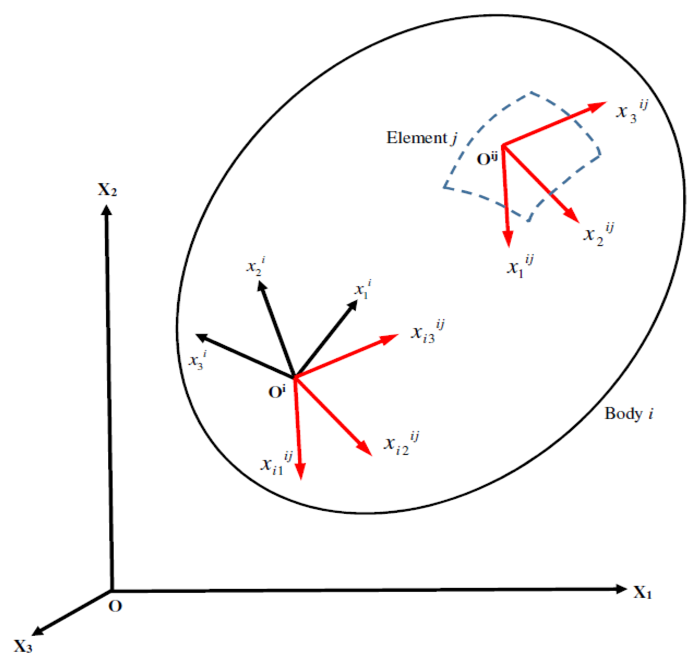
In the finite element formulation of the floating frame of reference formulation, four coordinate systems are used as shown in
Figure 6—(1) the global coordinate system
X1X2X3, (2) the body
i coordinate system
, (3) the element coordinate system
and (4) the intermediate element coordinate system
. The global coordinate system is inertially fixed. The body
i coordinate system, one in each body
i, is not rigidly attached to a point in the body. The element coordinate system, one in each element, has an origin rigidly attached to a point in the element. As a result, it translates and rotates with the element. The intermediate element coordinate system, one in each element, has an origin rigidly attached to the origin of the body
i coordinate system
Oi. This coordinate system has a fixed orientation with respect to the body
i coordinate system. Its orientation is selected such that it is initially parallel to the axes of the element coordinate system.
The displacement field in the element
j expressed in the body
i coordinate system is:
where:
and
is the vector of nodal coordinates in the body
i, that is,
For a 2D beam element, that is, a beam element with only longitudinal and transversal translations and a rotation about its longitudinal axis,
where
βij is the fixed angle between the intermediate element coordinate system and the body coordinate system. In other words, the matrix
Cij is the constant rotation matrix between the intermediate element coordinate frame and the body coordinate frame. In a planar case, the matrix
Cij is a 2 × 2 elementary rotation matrix such as that given in Equation (112). In a spatial case, the matrix
Cij is a 3 × 3 rotation matrix.
The matrix
is a Boolean matrix defined for each element with respect to the body
i nodal coordinates
to establish a connectivity between elements in that body:
Similar to Equation (2), the body
i nodal coordinates
can be written as:
where
is the vector of undeformed nodal coordinates in the body
i whereas
is the vector of elastic nodal deformations in the body
i before any boundary condition is applied. Due to a set of applied boundary conditions, the vector
is reduced to the vector
. This reduction can be conveniently written as:
where the matrix
is a Boolean matrix.
6.1. Formulation at the Element Level
The inertia matrix of an element is given by the following symmetric matrix:
where:
For a 2D beam element with length
lij, the matrices
,
and
are given by:
The stiffness matrix of an element is:
where:
6.2. Formulation at the Body Level
The inertia matrix of a body
i, before the application of any boundary condition, is the following symmetric matrix:
The stiffness matrix of a body
i, before the application of any boundary condition, is:
where:
The process of assembly indicated in Equations (131) and (133) is conducted by overlapping the elements of the matrices corresponding to the nodes of connectivity between elements, as well-known in the finite element method. The notation ne in Equations (131) and (133) denotes the number of elements in the body i. Upon the application of a set of boundary conditions, the inertia and stiffness matrices are reduced to and . This reduction can be easily conducted by suppressing the rows and columns corresponding to the constrained elastic coordinates. It should be noticed that the assembly of the elements and the suppression of the rows and columns corresponding to the constrained elastic coordinates are conducted at the body level.
The quadratic velocity vector, the gravitational force vector and the external force vector in the body i consist of their rigid and elastic components and are defined as in Equations (30), (33) and (35), respectively. The matrix B for the body i can be obtained by using Equation (40).
6.3. Formulation at the System Level
The inertia and stiffness matrices of the system after the application of the boundary conditions are:
The matrices and have an identical dimension. The notation nb in Equations (134) and (135) denotes the number of bodies in the system.
The EOMs of the system are given by DAEs as in Equations (43) and (44). The expanded expression of the EOMs showing its rigid and elastic components is provided in Equation (88).
7. Flexible Body Dynamics Based on Finite Element Approximation
Using a 2D Euler-Bernoulli beam model as in the Rayleigh-Ritz approximation previously discussed, let’s discretize each of the four bodies in the manipulator into four elements with equal lengths, that is,
As a result, there are five nodes in each body. All the nodes along with the nodal coordinates in each body
i, before the application of any boundary condition, is depicted in
Figure 7. The nodes 2–4 are the nodes of connectivity at which two adjacent elements are connected.
As the manipulator at hand has four bodies (links), the nodal coordinates in the system are given by:
The sub-vector
in Equation (142) has a dimension of 5 × 3 = 15 as there are 5 nodes in each body
i with 3 DOFs in each node, that is,
The dynamics of the manipulator at hand is constrained by nine position constraint equations. Three of them are position constraints corresponding to the three rigid sliders as given in Equations (64)–(66). The rest of the position constraints are as follow:
where:
The fixed-free elastic boundary conditions, identical to that in the Rayleigh-Ritz approximation, are used. These boundary conditions constrain all the elastic DOFs in the first nodes of each body and let the remaining elastic DOFs free. As a consequence, all the matrices and vectors for each body should be reduced by suppressing the rows (for the case of vectors) and rows and columns (for the case of matrices) corresponding to the constrained elastic DOFs. This results in a dimensional reduction of the elastic matrices and vectors for each body from 15 to 12. This suppression is expressed in Equation (117). For the fixed-free boundary conditions, this can be written for each body
i as:
Accordingly, the dimension of the system is also reduced. The EOMs of the system are written as Equation (88) with the generalized coordinates q defined in Equations (89) and (90) but now the elastic coordinates for each body are given by Equation (156).
8. Numerical Results
8.1. Manipulator Parameters
Given the manipulator at hand with legs having length of L1 = 486 mm, L2 = 500 mm and L3 = 507 mm. The moving platform has dimensions of xp2 = xp3 = xp = 315 mm. Hence, two upper revolute joints are coincident. The COM of the legs are L1G = 199 mm, L2G = 244.8685 mm and L3G = 238.9118 mm whereas the COM of the moving platform is xPG = 165.9629 mm. The masses of all of the sliders, all of the three legs and the moving platform are ms1 = ms2 = ms3 = 7 kg, mL1 = 8.5 kg, mL2 = 9.8470 kg, mL3 = 10.8420 kg and mp = 15.2425 kg, respectively. The mass moments of inertia of the legs with respect to their COM are given by IG1 = 0.1673 kg m2, IG2 = 0.2051 kg m2 and IG3 = 0.2322 kg m2, whereas the mass moment of inertia of the moving platform with respect to its COM is given by IGp = 0.1260 kg m2. All the links have an identical modulus of elasticity E = 7.0 × 10¹⁰ Pa and an identical rectangular cross section of b × h = 150 × 50 mm. Assuming that the manipulator is on XY plane (and accordingly the gravity applies), the depth b of 150 mm is measured in z-direction (perpendicular to the paper) whereas the depth h of 50 mm is measured on XY plane (on the paper plane). It is assumed that there is no friction at all the joints.
8.2. Input Forces and Elastic Coordinate Boundary Condition
Two different types of loads namely sinusoidal and triangular pulse loads are applied to the active joints of the manipulator. The sinusoidal loads are given by:
whereas the triangular pulse loads ramp up from zero at
t = 0 to respectively 10 N, −2 N and −2 N for the three sliders at
t = 0.1 s and ramp down to zero at
t = 0.2 s. It should be noticed that the manipulator will keep moving after the triangular pulse loads ramp to zero due to the gravity. The elastic displacement is evaluated by applying fixed-free boundary conditions to each link.
8.3. Solutions
Since the DAEs representing the dynamics of the manipulator are transformed to ordinary differential equations (ODEs) through partitioning, the solution can be easily obtained by integrating the ODEs. The second order ODEs were transformed to a state space representation as described earlier and subsequently integrated numerically by using MATLAB ODE45. The integration was performed within 0 to 4 s.
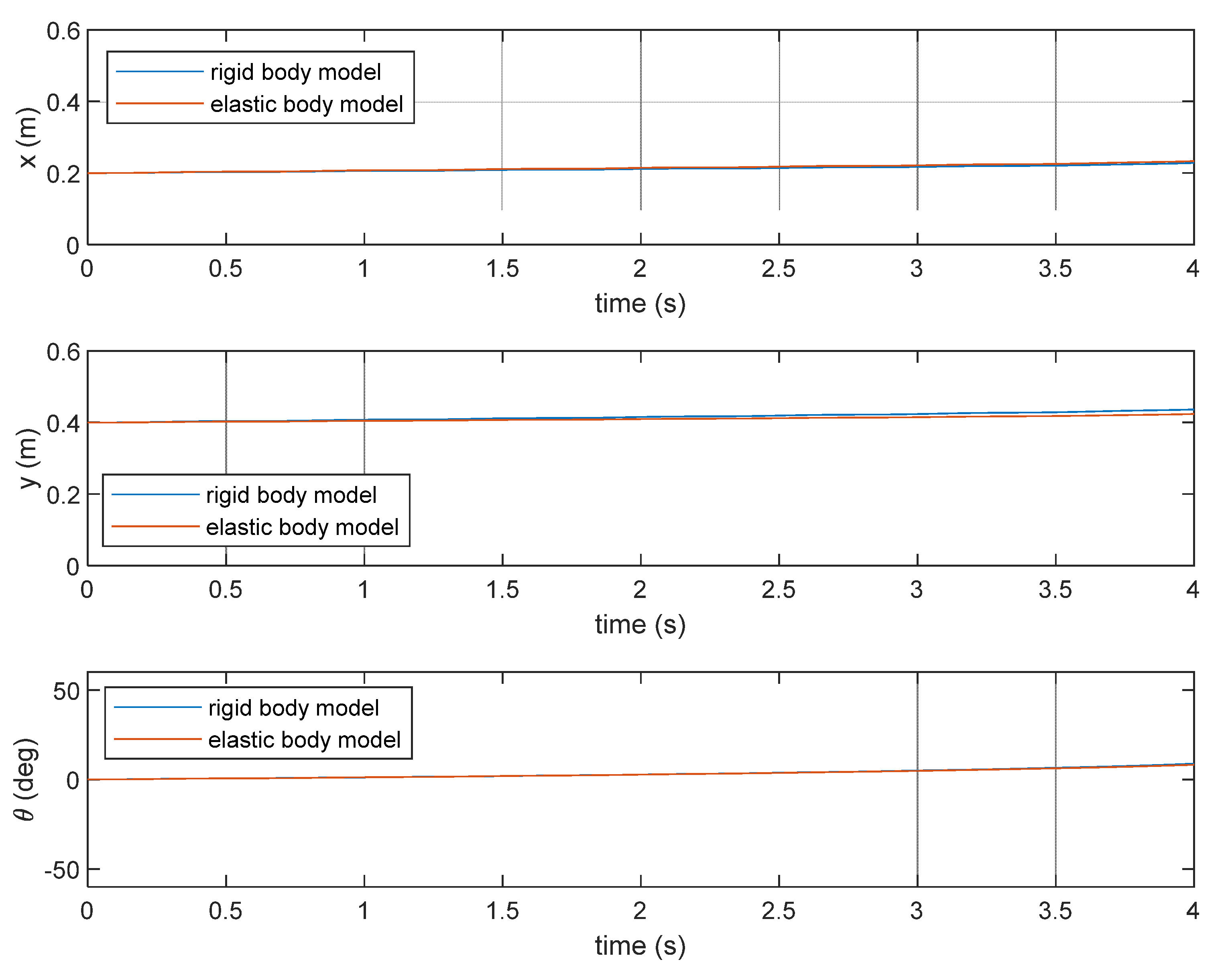
Figure 8 and
Figure 9 show the end-effector position and orientation of the manipulator subject to the sinusoidal loads. Both figures depict the end-effector position and orientation of the manipulator modeled as rigid body and flexible body. The flexible body model used in
Figure 8 is based on the Rayleigh-Ritz method whereas that used in
Figure 9 is based on the finite element method.
For more clarity,
Figure 10 shows the elastic displacements as well as the orientation of the end effector evaluated by using the two methods in the case of sinusoidal loads.
Figure 11 shows the elastic displacements as well as the orientation of the end effector evaluated by using the two methods in the case of the triangular pulse loads. It should be noticed that the orientation plots shown in
Figure 10 and
Figure 11 indicate the absolute orientation values of the manipulator with flexibility of all the links taken into account, not the elastic displacements alone. It is shown that the flexibility of the manipulator links results in infinitesimal displacement in both the translational DOFs and the rotational DOF in addition to the rigid body displacement of the end-effector. This infinitesimal displacement should be taken into account when dealing with a high precision application such as machining. Furthermore, it is shown that the elastic displacement obtained by both the methods have some degree of agreement, with some difference in the magnitude.
It can also be seen that the elastic displacements in the y-direction is larger than that in the x-direction. The former is roughly twice the latter. This can be related to the manipulator stiffness. The larger elastic displacement in the y-direction might be caused by smaller manipulator stiffness in the y-direction. This can be due to less depth of the manipulator in the y-direction compared to its depth in the x-direction during the performed motion. In fact, the stiffness of the manipulator in the y-direction is at its best when the manipulator is standing tall and therefore has a large depth in the y-direction. In such a posture, the stiffness in the x-direction will be reduced. The varying stiffness corresponding with the changing posture is a typical characteristics of parallel manipulators.
Moreover, the magnitude of the elastic displacements which represents the flexibility of the manipulator is shown to be unrelated with the methods as it is shown that the finite element method gives fewer elastic displacements in the case of sinusoidal loading but it gives larger elastic translational displacements in the case of triangular pulse loading. This implies an inconsistent relation between the flexibility of the manipulator and both the methods given a variety of loadings.
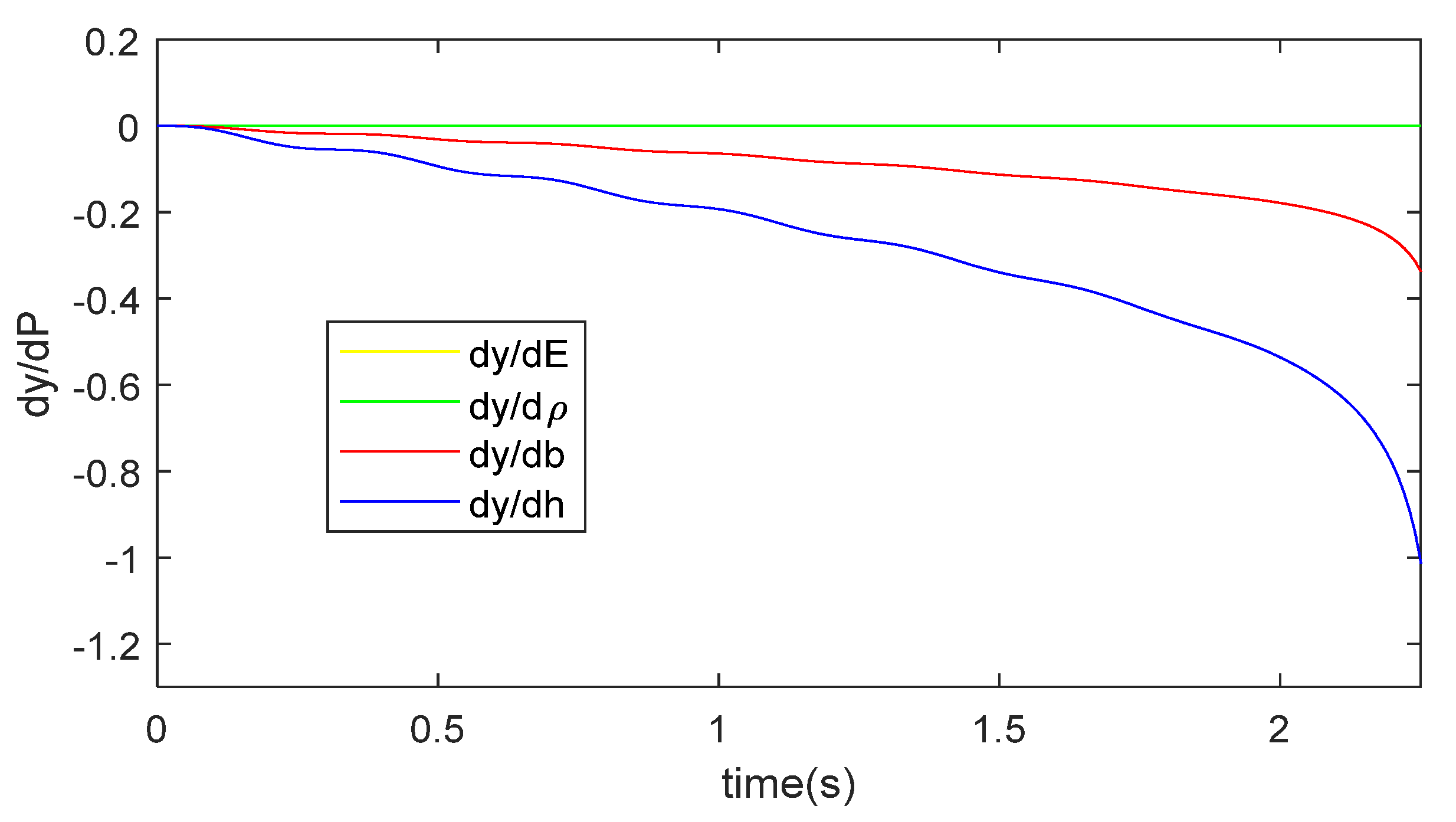
8.4. Sensitivity Analysis
The sensitivity of the displacements x, y and θ with respect to the design parameters was analyzed by evaluating the gradients of those displacements with respect to the design parameters. As all the links of the manipulator are designed to have the same material, the inertial and elasticity properties of the links are dependent on the mass density and the modulus of elasticity E of the links, respectively. Other design parameters affecting both the mass and the elasticity of the links are the cross section geometry. As the links in this case have a rectangular cross section, these parameters are the width b and height h of the rectangular cross section. Thus, the design parameters are P = {E, , b, h}. The gradients of the displacements with respect to the aforementioned design parameters were obtained by using finite difference approach. The difference between the displacements corresponding to perturbed design parameters and the displacements corresponding to unperturbed design parameters is divided by the amount of perturbation. Using SI units for all the design parameters, a perturbation of 1 × 10⁻⁵ was used for all the design parameters.
Figure 12,
Figure 13 and
Figure 14 show respectively the sensitivity of the displacements
x,
y and
θ with respect to the design parameters. All the figures show that the displacements in all the DOFs are more sensitive to the dimension of the cross section than to both the modulus of elasticity and the mass density of the links material. Furthermore, the displacements in all the DOFs are more sensitive to the height
h of the cross section than to the width
b of the cross section. This is expected as the manipulator is working on the XY plane which is the plane where the height
h is defined. In this case, the area moments of inertia of the links, which affect the elasticity of the links, have a cubic relation with the height
h and have a linear relation with the width
b of the cross section. Hence, a change in the height
h will affect more the elasticity of the links than a change of the width
b. Consequently, the rigidity of the links can be significantly increased by increasing the height
h of the links’ cross section.
9. Conclusions
A more realistic model of a flexible parallel manipulator was presented in this paper by assuming that all the links, including the moving platform, are flexible. Since the moving platform connects the end-effector to the legs, in general its flexibility should be taken into account in order to obtain a more accurate end-effector position. Furthermore, the non-symmetry of the manipulator represents a more general topology of planar parallel manipulators. The simulation using both the Rayleigh-Ritz and finite element approximations, as expected, showed that the manipulator undergoes a larger displacement when the link flexibility is taken into account. The comparison between both approximations using Euler-Bernoulli beam to model the links, which is the main contribution of this paper, showed an agreement in the direction and rough magnitude of the elastic displacement. The agreement between the two methods verifies each other. This can serve as a base to use only the finite element method using FFRF framework in the future to evaluate the elastic displacements of the manipulator at hand with complex geometry of the links. In such a case, appropriate 3D finite elements should be used to adequately represent the complex geometry. The huge number of DOFs resulting from the use of 3D finite elements can be reduced, if required, by employing a model order reduction technique. Finally, based on the sensitivity analysis, the rigidity of the links of the manipulator at hand can be significantly increased by increasing the height h of the links’ cross section.


