Potential of Supercritical Carbon Dioxide Power Cycles to Reduce the Levelised Cost of Electricity of Contemporary Concentrated Solar Power Plants

Featured Application

Assessment of the potential of supercritical Carbon Dioxide power cycles to reduce the Levelised Cost of Electricity of contemporary Concentrated Solar Power plants, with the aim to benchmark the cost of electricity of the current and next generation Concentrated Solar Power (CSP) technology.

Abstract

This paper provides an assessment of the expected Levelised Cost of Electricity enabled by Concentrated Solar Power plants based on Supercritical Carbon Dioxide (sCO${}_2$) technology. A global approach is presented, relying on previous results by the authors in order to ascertain whether these innovative power cycles have the potential to achieve the very low costs of electricity reported in the literature. From a previous thermodynamic analysis of sCO${}_2$ cycles, three layouts are shortlisted and their installation costs are compared prior to assessing the corresponding cost of electricity. Amongst them, the Transcritical layout is then discarded due to the virtually impossible implementation in locations with high ambient temperature. The remaining layouts, Allam and Partial Cooling are then modelled and their Levelised Cost of Electricity is calculated for a number of cases and two different locations in North America. Each case is characterised by a different dispatch control scheme and set of financial assumptions. A Concentrated Solar Power plant based on steam turbine technology is also added to the assessment for the sake of comparison. The analysis yields electricity costs varying in the range from 8 to over 11 ¢/kWh, which is near but definitely not below the 6 ¢/kWh target set forth by different administrations. Nevertheless, in spite of the results, a review of the conservative assumptions adopted in the analysis suggests that attaining costs substantially lower than this is very likely. In other words, the results presented in this paper can be taken as an upper limit of the economic performance attainable by Supercritical Carbon Dioxide in Concentrated Solar Power applications.

1. Introduction

1.1. Current Status of Concentrated Solar Power Technology. Expectations Raised by Supercritical Carbon Dioxide Power Cycles

Supercritical Carbon Dioxide power cycles are currently seen as the technology of choice for next generation Concentrated Solar Power plants to produce Solar Thermal Electricity (STE). They promise higher efficiencies than state-of-the-art Concentrated Solar Power (CSP)-STE facilities based on steam technology, and they are reportedly much more compact thanks to the higher density of the working fluid and the simpler layout of the working cycle. Nevertheless, this latter feature, compactness of the power block, does not constitute an essential difference with respect to conventional steam technology, given that the power block contributes a fairly small fraction to the land area occupied by a Concentrated Solar Power plant. On the contrary, the higher efficiency of sCO${}_2$ systems (as compared to contemporary technology) reduces the heat input needed for a given power output and thermal energy storage capacity, which translates into a smaller solar field and TES system. This turns out to be crucial for reducing both the footprint and cost of this new generation of CSP-STE systems based on sCO${}_2$.

In 2011, the SunShot programme, flagship R&D instrument of the United States Department of Energy to foster the development of solar power generation, set the objective to reduce the cost of solar electricity to 6 ¢/kWh in 2020. This ambitious objective was already achieved in 2017 by photovoltaic technology in large-scale facilities, and it has been superseded by a much more ambitious goal of 3 ¢/kWh in 2030. Unfortunately, whilst PV is now cost-effective and competitive against other renewable and non-renewable technologies, even in smaller domestic applications, it looks like CSP-STE is experiencing more difficulties to meet these objectives with the technology currently available. This is where the cumulative cost reduction potential brought about by sCO${}_2$ power cycles in combination with more mature solar field and thermal energy storage technologies, along with the exploitation of economies of scale of the CSP industry, comes in to pave the way for a drastic cost reduction of Solar Thermal Electricity. Figure 1, adapted from the information made public by Solar Energy Technologies Office of the Department of Energy [1], provides this roadmap for CSP-STE technologies.

Figure 1. Progress and goals for Solar Thermal Electricity set by the SunShot programme. Data obtained from [1].

1.2. Technical Hurdles Hindering the Development of Supercritical Carbon Dioxide Power Cycles for CSP Applications

Unfortunately, even if the advent of supercritical Carbon Dioxide technologies in the beginning of the twenty-first century was seen as the perfect opportunity for a drastic cost reduction of CSP-STE, this perception has not materialised. The large research efforts needed to develop the technology, hence reducing the associated capital cost, and the much slower pace at which CSP is being deployed to the market, are hindering the construction of a first commercial (or even pre-commercial) plant demonstrating the concept. Moreover, in recent years, much more attention has been put on a seemingly unsolvable problem in the low temperature section of the sCO${}_2$ cycle, which is the thermodynamic cornerstone of the reportedly better performance of this cycle with respect to conventional steam cycles.

The realisation of efficient supercritical CO${}_2$ power cycles requires that the inlet temperature to the compressor be close to, or even lower than, the critical temperature of this fluid (≈31 °C). When this is possible, and if the peak temperature of the cycle is higher than 600–650 °C, then the sCO${}_2$ cycle outperforms any Rankine cycle running on water/steam with the same boundary conditions. Unfortunately, CSP plants are typically located in arid sites with ambient temperatures well above 35 °C, which makes it impossible to cool the cycle down to the temperatures needed to compress the fluid in the vicinity of the critical point (there where density is very high) with low power requirements. Accordingly, the rapid transition to an almost ideal behaviour of Carbon Dioxide when temperature increases to 40 °C or above increases compression work and reduces the thermal efficiency of the power block, which can only be increased again through a large increase of turbine inlet temperature. Of course, this poses new challenges in the area of receiver technology, heat transfer fluids and materials, and also brings about higher costs.

In order to overcome these thermodynamic problems, the SCARABEUS formulates a new conceptual approach to sCO${}_2$ cycles whereby the composition of the working fluid is tailored to the high ambient temperatures typically found in CSP sites. This is enabled by the addition of certain dopants with higher critical temperature than Carbon Dioxide to the raw CO${}_2$ used in standard sCO${}_2$ cycles. The addition of these dopants increases the critical temperature of the mixture and enables liquid-like compression (in supercritical conditions) even at ambient temperatures as high as 40–45 °C or even 70 °C. The concept has already been formulated by partners of the consortium in [2,3], showing promising results, but it is too early to assess the impact of this new technology on the economic performance of CSP-STE. New equipment (turbomachinery and heat exchangers) is needed and the properties and thermal stability of the dopants considered must be confirmed in long-term operation at high temperature. This falls within the scope of the SCARABEUS project and more information will be presented in the near future.

1.3. Objectives and Novelty. Benchmarking the First Generation of CSP-sCO${}_2$ Power Plants

Akin to what was done several years ago to benchmark the then innovative supercritical Carbon Dioxide cycles in Concentrated Solar Power applications, a new reference is now needed to understand whether or not the SCARABEUS technology will eventually yield lower Levelised Cost of Electricity than standard sCO${}_2$ power cycles. This encapsulates the twofold objective of the present work, in brief: (i) to produce accurate estimates of the Levelised Cost of Electricity that is attainable for Concentrated Solar Power plants using supercritical CO${}_2$ cycles; and (ii) to provide a benchmark for the innovative SCARABEUS technology currently under development.

In this regard, the authors of this paper have carried out an ambitious research to assess the true potential of sCO${}_2$ power cycles, with the aim to provide a structured pathway for the thermo-economic feasibility analysis of this technology when applied to CSP power plants. The results of this research have been published regularly in the last four years, and the present paper represents the last, wrap-up piece of the process. The research starts with a very thorough review of the technical (scientific and industrial) works dealing with sCO${}_2$ technologies [4]. Since the early works by Sulzer, Angelino and Feher [5,6,7], this work provides a comprehensive classification of virtually all the cycle layouts found in the literature with the aim to facilitate the comparison between different layouts. Amongst all these cycles, the twelve candidates fitting best into CSP applications are shortlisted for a rigorous and systematic thermodynamic analysis in [8], with the goal to assess their true potential, free from the inherent technical constraints brought about by contemporary technology-related limitations. The thermodynamic assessment presented in [8] is complemented by two additional papers by the authors, [9,10], aimed at assessing the expected component cost of each major equipment in the plant in order to estimate the installation costs of CSP plants using sCO${}_2$ power cycles. Out of this analysis, two of the twelve configurations are found to provide the best thermal and economic performance: Allam and Partial Cooling. For these two layouts, dedicated models of performance to assess the corresponding off-design performance are developed with the aim to calculate the annual production of electricity (annual yield) for a particular location and set of boundary conditions [11].

With all the information described above, this paper constitutes the last step in this research, leading to the original objective of estimating the Levelised Cost of Electricity f CSP-sCO${}_2$ power plants. As said before, this is the Key Performance Indicator needed to assess whether or not standard sCO${}_2$ cycles or the new SCARABEUS concept will enable meeting the ambitious LCoE objective set forth by the SunShot programme. The value of the present paper lies on two main features. First, the wide portfolio of cycle layouts as produced by the review paper written by the authors in 2017 based on 160 references [4], which ensures that all the candidate cycles are included in the comparison. Second, the fact that the series of papers listed in the previous paragraphs are all consistent in the methodologies used and assumptions made. Indeed, each piece of research is built upon a previous one by the authors and, therefore, the thermodynamic references and environmental conditions are all consistent, the time value of money is taken into account to normalise currency, the on and off-design models of performance used to calculate the yield of each cycle are the same, and there is no bias in the comparative analysis of results. This applies to the entire process, from literature review to LCoE calculation.

2. Techno-Economic Assessment of CSP Based on sCO${}_2$

2.1. Operating Conditions

The initial works on supercritical power cycles acknowledged the superior thermal performance of this technology, with respect to standard steam cycles, when turbine inlet temperatures are higher than 600/650 °C [6]. Below this value, the little gain (if any) brought about by sCO${}_2$ cycles does not pay off the lower reliability and higher cost of a still less mature technology. Unfortunately, even at the lower end of the temperature range where sCO${}_2$ is substantially better than steam, the operating temperatures that are needed are far from the values currently achieved by commercial solar technologies, as recently confirmed by a report issued by the SCARABEUS consortium [12]. Two major hurdles are identified. Receiver technologies able to achieve temperatures in excess of 700 °C are available but they have not reached the commercial stage yet [13]. This also applies to heat transfer fluids able to harvest this high-temperature thermal energy available in the receiver, in order to feed both the power block and Thermal Energy Storage system, which are currently available but not widely commercialised [14]. This availability of high temperature heat transfer fluids is assessed in Table 1 where the characteristics of different intermediate to high-temperature molten salts are listed. Amongst them, this work makes use of FLiNaK for the sake of continuity with past works by the authors. Thermodynamic-wise, this is a very interesting option even though the very high cost of this salt compromises the economic feasibility of its practical implementation. Still, it is assumed that adopting this fluid yields a safe (conservative) estimate of the cost of electricity associated to this technology.

Table 1. Comparison between different molten salts for intermediate-high temperature Concentrated Solar Power (CSP) plants.

Salt	Composition [%]	Freezing Point [°C]	Boiling Point [°C]	Price [$/kg]	Price [$/kWh${}_{\mathit{t}}$] *
NaNO${}_3$-KNO${}_3$ (Solar Salt) [15]	60–40	220	600	0.8	10
LiF-NaF-KF (FLiNaK) [14]	46.5–11.5–42	454	1570	8.6 [16]	54.8
Li${}_2$CO${}_3$-Na${}_2$CO${}_3$-K${}_2$CO${}_3$ [17]	32–33–35	397	662	2.5 [15]	26.1
Na${}_2$CO${}_3$-NaOH [17]	19–81	284	714	-	2.3
MgCl${}_2$-KCl [15]	37.5–62.5	426	1412	0.35	5
ZnCl-NaCl-KCl [15]	69–7–24	204	732	0.8	18

* Values taken from [15] are obtained for $\Delta T_{salt}$ = 200 °C. For the FLiNaK, authors calculated this price for $\Delta T_{salt}$ = 290 °C. Values taken from [17] are estimated with market price of raw components in Q1 2015, for a maximum cycle temperature of 650 °C.

The thermodynamic potential of sCO${}_2$ power cycles for different boundary conditions and applications was assessed by the authors in a previous work [8], based on an earlier, thorough literature review [4]. In a second step, turbine inlet temperature was set to 750 °C, based on several works in literature [18,19] and on private communications with Abengoa (a SCARABEUS partner), and the assessment of thermal performance was complemented by an economic analysis with the aim to calculate the capital cost of a representative CSP plant using each cycle layout [10]. The main specifications of this reference plant are presented in Table 2.

Table 2. Specifications of the reference sCO${}_2$ power plant.

Net Power Output	${\mathit{P}}_{\mathit{max},{\mathit{sCO}}_2}$	TIT	TES${}_{\mathit{capacity}}$	SM	DNI${}_{\mathit{nom}}$	${\mathit{T}}_{\mathit{amb},\mathit{nom}}$
[MWe]	[MPa]	[°C]	[hour]	[-]	[W/m${}^2$]	[°C]
50	30	750	10	2.4	850	15

The thermo-economic performance of the reference power plant in Table 2 considering different cycle layouts is presented in Figure 2 for a pressure range deemed affordable in the medium term (15 to 40 MPa). Akin to the results provided in [8], ${\eta }_{th}$ presents an increasing trend with pressure up 35 MPa. This is common to all cycles except the Recompression cycle (RC), in which the efficiency peaks a little sooner (30 MPa). On the other hand, the minimum Overnight Capital Cost is found between 30 and 35 MPa for all the cycles considered. Based on this, turbine inlet pressure is set to 30 MPa in the reference CSP plant, since this yields the best compromise between thermodynamic and economic performances and has already been proven to be achievable in similar power technologies such as ultra-supercritical steam turbines [20].

Figure 2. Effect of maximum cycle pressure on thermal efficiency and Overnight Capital Cost per kilowatt. Legend: Simple Recuperated (SR), Transcritical (TC), Partial Cooling (PC), Recompression (R), Pre-compression (PrC) and Allam (Al). Data adapted from [10].

2.2. Economic Assessment

The calculations presented in Figure 2b above account for uncertainty regarding the capital costs of components. Using a Montecarlo analysis, each component cost is assigned a probability density function whereby costs are randomly taken from a given range of values with different probability: the cost of components with a lower maturity are allowed to change in a wider range whereas this range is much narrower for well established technologies. According to these calculations, uncertainty can potentially change the capital cost of the power block by plus/minus one-third of the cost, which is aligned with the information provided in the work by Weiland et al. for the National Energy Technology Laboratory and Sandia National Laboratories in the USA. In this latter work, the authors relied on data provided by Original Equipment Manufacturers to estimate the installation costs of small and large power plants operating on gaseous and solid fossil fuels [21]. The results, which also accounted for uncertainty of the input data provided by vendors, were similar to those reported in [10] both in terms of the total values and the variability brought about by uncertainty. As discussed by Carlson et al., this is very likely due to the lack of a well established market that prevents engineering costs from being charged on very few clients [22].

The data presented in Figure 2 in the previous section are expanded in Table 3, the economic values of which are calculated for the 85% confidence interval based on the probability density functions discussed in [10]. The table provides information about the main thermodynamic features—thermal efficiency (${\eta }_{th}$) and temperature rise across the solar receiver ($\Delta T_{solar}$)—and about the Overnight Capital Cost of the plant and the contribution of each major equipment (TES, Solar Field, Tower/Receiver and Power Block). According to these data, the Transcritical CO${}_2$ (TC) and Recompression (RC) layouts yield the lowest and highest installation costs, respectively, 5656 and 6867 $\$/k{W}_{inst}$, while the Partial Cooling (PC) cycle seems to provide the best compromise between thermal and economic features, closely followed by the Allam (Al) cycle.

Table 3. Thermo-economic assessment of different cycle layouts. Adapted from [10].

Cycle	${\mathit{\eta }}_{\mathit{th}}$	$\mathbf{\Delta }{\mathit{T}}_{\mathit{solar}}$	OCC	${\mathit{C}}_{\mathit{TES}}$	${\mathit{C}}_{\mathit{SF}}$	${\mathit{C}}_{\mathit{T}\&\mathit{R}}$	${\mathit{C}}_{\mathit{PB}}$
	[%]	[°C]	[$/kW${}_{\mathit{inst}}$]	[k$]	[k$]	[k$]	[k$]
SR	45.8	290	6404	78,184	85,657	75,123	50,585
TC	48.3	290	5656	76,648	80,675	75,307	21,896
PrC	50.6	254	6515	80,145	76,373	79,697	58,835
RC	50.5	220	6867	91,640	76,547	90,000	52,498
PC	51.1	290	5907	70,230	75,603	70,945	50,568
Al	45.0	290	5943	79,403	87,074	75,778	26,227

The information shown so far confirms that the installation costs based on sCO${}_2$ power cycles are comparable or even lower (for some layouts) than for steam turbines used in state-of-the-art CSP plants −5800 $\$/k{W}_{inst}$ according to [23]. The large cost share of the Thermal Energy Storage system is also confirmed, which puts the temperature rise across the solar receiver stems forward as a critical factor involved in plant design, given its very strong impact on the inventory of salts that is needed to operate a plant of given output and storage capacity. Finally, heat exchangers stem as the most relevant individual component in the power block cost-wise, Figure 3, with a larger share than turbomachinery; this confirms earlier comments in this section.

Figure 3. Breakdown of the Overnight Capital Cost of the power block.

A closer look into the operation of the cycles compared in Table 3 reveals that the Transcritical CO${}_2$ cycle requires the most restricting boundary conditions in order to achieve the lowest installation costs in the list. This is due to the need to enable condensation of the working fluid, which is only possible if the inlet temperature to the Transcritical CO${}_2$ pump is set to about 15 °C (strictly speaking, a temperature lower than the critical temperature of CO${}_2$ would suffice to enable the implementation of a Transcritical cycle. Nevertheless, performance-wise, this layout only makes sense if the saturation temperature in the condenser is substantially lower than the critical temperature. This is why a value of 15 °C at the pump inlet is usually adopted). This translates into ambient temperatures in the order of 8 °C if an evaporative cooling tower is considered or less than 5 °C if air coolers are used, values that are only rarely found in the arid (even desertic) locations where CSP plants are typically found. The dismissal of the Transcritical CO${}_2$ layout for these reasons narrows the selection of cost-effective configurations to the Allam and Partial Cooling cycles, the layouts of which are presented in Figure 4. The main features of these cycles are:

Figure 4. Layouts of the Allam and Partial Cooling cycles.

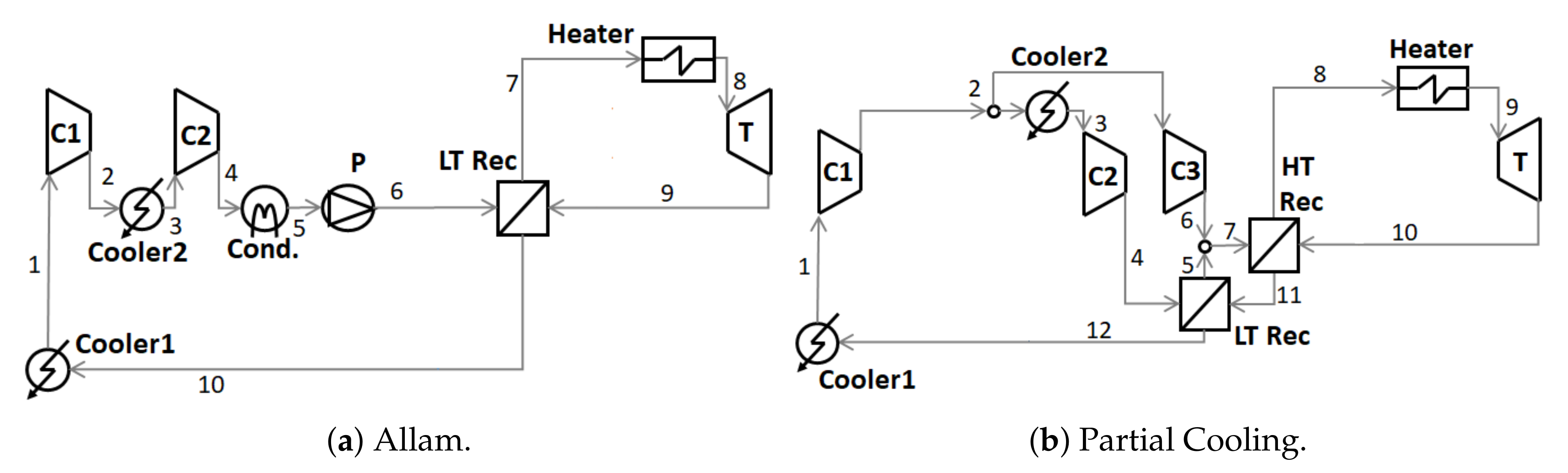
• Allam cycle: it is an extremely high recuperative cycle, an evolution of a standard Brayton cycle incorporating a three-step compression process with two compressors and a pump separated by an intercooler and a condenser respectively. Originally proposed by Allam [24] for oxy-combustion applications, this layout has been adapted considering pure sCO${}_2$ as working fluid [8].
• Partial Cooling cycles: this cycle derives directly from Angelino’s work [6], and it is an evolution of a Recompression cycle with the addition of a cooler and a pre-compressor before the flow-split. The most interesting features of the Partial Cooling cycle are its high specific work [25] and a very low sensitivity of global efficiency to deviations of pressure ratio from the optimum value [26].

The installation costs reported in Table 3 are presented graphically in Figure 3, showing that the high temperature heat exchanger (heat adder or heater) is the key contributor to installation costs, accounting for approximately half of the total OCC of the power block. This is due to the very high operating pressure and temperature of the sCO${}_2$-FLiNaK heat exchanger which, as a consequence, requires the utilisation of special alloys like Inconel 617 [10].

3. Levelised Cost of Electricity of CSP Plants Based on sCO${}_2$

3.1. Preliminary Notes on the Assessment of the Levelised Cost of Electricity ($LCoE$)

In addition to the installation costs presented in earlier sections of this paper, estimating the Levelised Cost of Electricity of CSP plants based on sCO${}_2$ technology requires a model to simulate the off-design performance of the power plant throughout the year. This provides the hourly output of the power plant for the specific boundary conditions—ambient temperature and pressure, available solar radiation, as described in [27] and, more recently [11]. The resulting information is then combined with the installation costs to obtain $LCoE$, as discussed in detail by M. Martin [13]. To this end, the authors have relied on the System Advisor Model SAM developed by the National Renewable Energy Laboratory of the United States’ Department of Energy, since this is widely accepted by the scientific community and already employed in cost estimation for sCO${}_2$ power plants [28,29].

The first part of this section describes the methodology used to incorporate the part-load performance of the Allam and Partial Cooling cycles into SAM’s calculation procedure. Then, this information is used to model the reference 50 MW CSP plant in Table 2, considering either of the cycles selected in the previous section. For each one, two different locations and four different combinations of financial parameters and dispatch control models are assessed. Finally, the results obtained are compared against a state-of-the-art CSP plant using a standard power block based on steam turbines.

The input parameters defining the solar field are set to their default values, meaning that the geometry of the field is optimised according to state-of-the-art specifications that are representative of the current industrial practice. The type and composition of the molten salt (or Heat Transfer Fluid considered) is selected in the Tower and Receiver menu, where either commercial solar salts (NaNO${}_3$KNO${}_3$) or FLiNaK can be selected. The latter is the same molten salt employed by the in-house models developed by the authors and it is therefore selected for this LCoE assessment.

For the power block, SAM is limited to the Recompression layout when it comes to power blocks based on supercritical CO${}_2$ systems, which is a strong limitation in this work. This is why the user-defined option is selected, which enables implementing the off-design performance of the Allam and Partial Cooling cycles modelled with the proprietary code developed by the authors and described in [11]. This is the step where the integration between SAM and the authors’ in-house codes actually takes place, enabling a much more detailed and flexible assessment of supercritical CO${}_2$ cycles than otherwise enabled by SAM. This integration requires the following specific information, in addition to more general technical features like the type of cooling system used (air or water cooled):

• MOD1-Performance as a function of HTF temperature: the part-load performance of the power cycle for variable molten salt (hot) temperature is obtained for three normalised mass flow rates of molten salts, in this case: 0.2, 1 and 1.05. The rated hot temperature of molten salts is set to 770 °C and this parameter is varied between 700 and 800 °C in the analysis.
• MOD2-Performance as a function of HTF mass flow rate: the part-load performance of the power cycles for variable mass flow rate of molten salts is obtained for three values of ambient temperature, in this case: 5, 15 and 40 °C. To this end, the same range of normalised mass flow rate as in the previous bullet point is considered; i.e., between 20% and 105% of the rated mass flow rate of FLiNaK.
• MOD3-Performance as a function of ambient temperature: the part-load performance of the power cycles is obtained when ambient temperature varies between 5 and 40 °C. Again, three molten salt (hot) temperatures are considered: 700, 770 and 800 °C.

The MOD-1 to MOD-3 tables corresponding to the reference power plant based on the Allam and Partial Cooling cycles are provided in Appendix A. They contain information about the specific off-design cycle performance considered in the simulations leading to the calculation of the Levelised Cost of Electricity and, therefore, they are deemed very valuable in terms of credibility of the work. The following list clarifies each parameter reported in Appendix A:

• Net electric output (${\dot{W}}_{cycle}$): power output at generator terminals minus auxiliary power consumption. Auxiliary power accounts for the power needed to drive auxiliary equipment in the power block.
• Heat input ($Q_{in}$): heat supplied to the power block (i.e., absorbed by the working fluid).
• Power consumption of the cooling system (${\dot{W}}_{cooling}$): power consumed by the evaporative cooling system.
• Water mass flow rate of the cooling system (${\dot{m}}_{w,cooling}$): total amount of water needed in the cooling system.

These parameters are obtained for the so-called best control strategy and they must be normalised with respect to their rated values. For a more detailed discussion about how the power cycles are operated off-design, interested readers are referred to a complementary work by the authors [11].

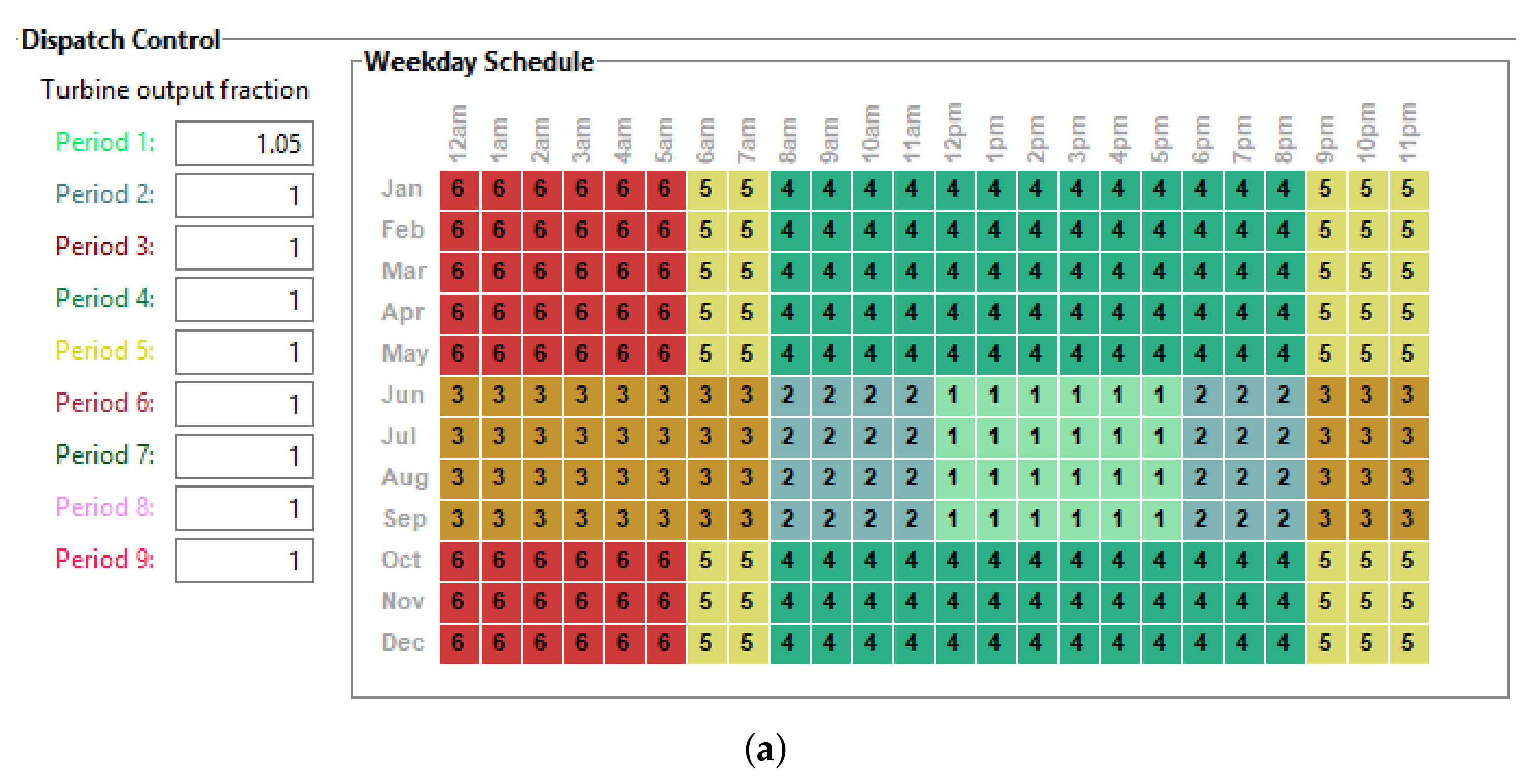
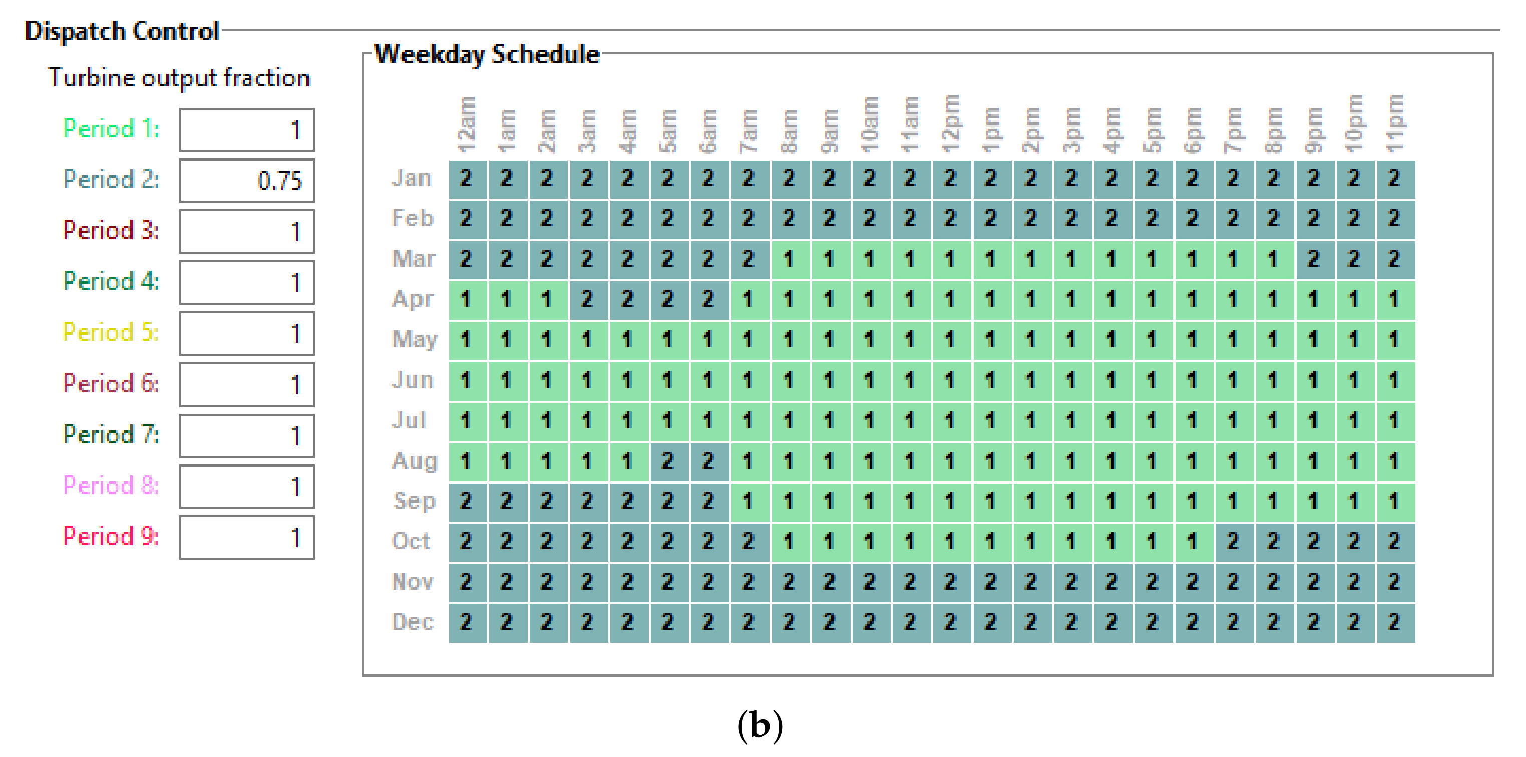
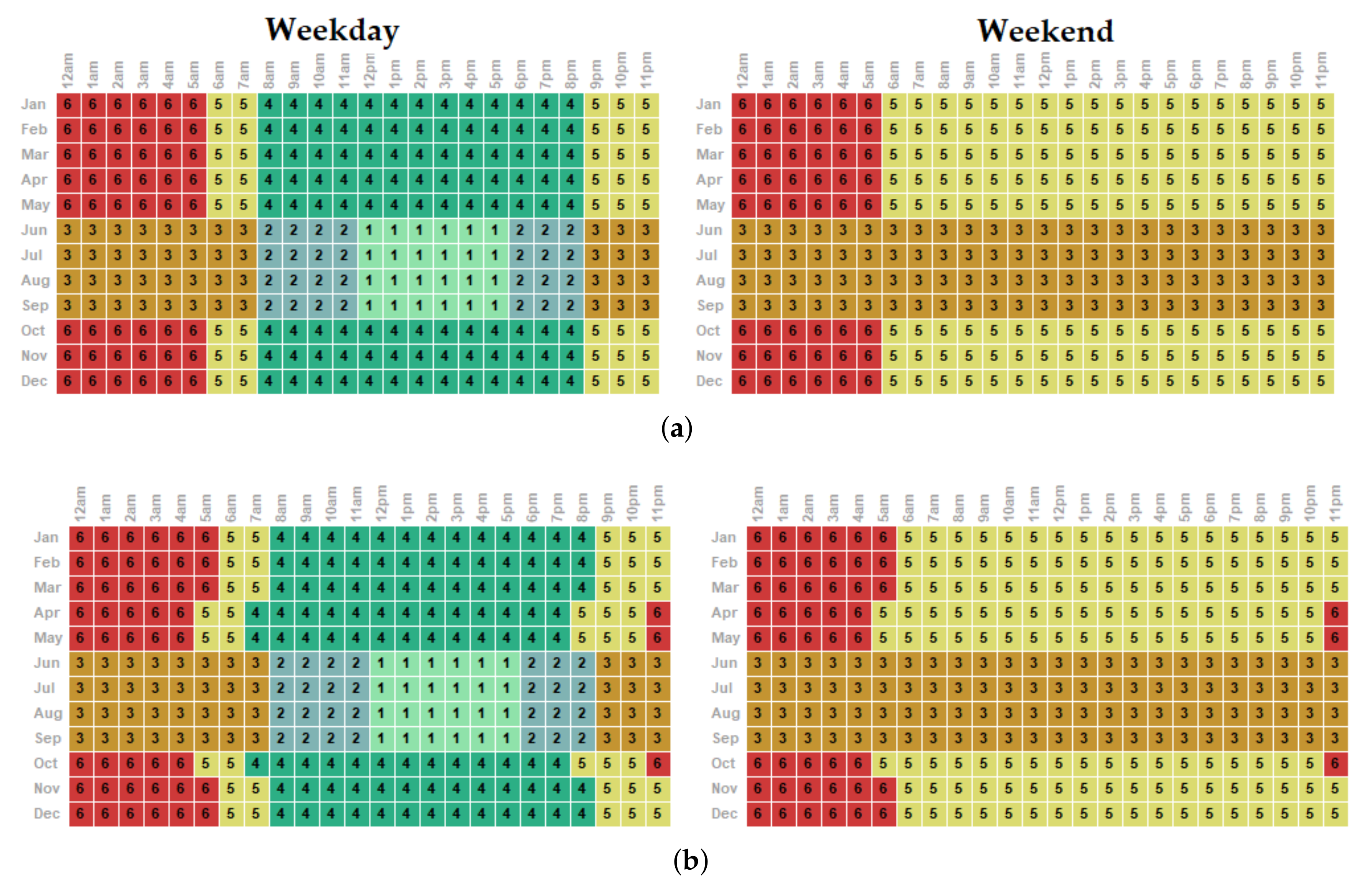
3.2. Dispatch Control and Financial Model

Dispatch control refers to the scheme under which the Thermal Energy Storage System and power block are operated. In other words, the periods and operating conditions during which the power block drains energy from the Thermal Energy Storage to make up for the lack of concentrated solar energy supplied from the solar field directly (in a power plant using molten salts, heat input to the power block is always provided by the Thermal Energy Storage system. The text refers to situations where the net energy balance in the Thermal Energy Storage systems is negative), in order to achieve the desired turbine output.

Two different dispatch control schemes are considered in this work: the default scheme reported by SAM and the scheme proposed by the SunShot Vision Study [28]. A graphical representation of these is presented in Figure 5 which confirms that these schemes merely define an overall schedule of plant operation but they do not substitute or interfere with the off-design control strategies described in another work from the same authors [11]. Actually, the control schemes are aimed at enabling the output setting assigned by the dispatchability scheme. In particular, for SAM’s default dispatch control, the plant runs at full capacity whenever possible, enabling a 5% over-charge during the central hours of the day in summer time, characterised by the highest solar irradiation. Running the plant in these conditions increases the average output of the plant but this is, potentially, at the cost of fewer operating hours in seasons with fewer sun hours. As opposed to this, the dispatch control scheme adopted by the SunShot Vision case drains energy from the Thermal Energy Storage system to sustain operation at 75% load during off-sun hours or during the day in seasons with lower solar radiation. This reduced load operation, marked in dark green (also number 2) in Figure 5, enables longer operating hours and reduces the number of shut-down/start-up manoeuvrers throughout the year.

Figure 5. Different dispatch controls used to assess the Levelised Cost of Electricity. (a) System advisor model’s (SAM’s) default dispatch control. (b) Dispatch control scheme for the SunShot Vision case [28].

The different sets of financial assumptions adopted by SAM and the SunShot Vision study are listed in Table 4. The information includes the target internal rate of return and time (year) when this should be achieved, lifetime of the project, inflation rate, nominal discount rate (also termed rate of return), debt ratio, payback time and interest rate. These parameters are needed to calculate the corresponding Power Purchase Agreement ($PPA$) required to meet the target IRR according to the remaining financial settings. This $PPA$ is actually another difference between the financial models based on SAM’s and Sunshot cases, in particular regarding the Time-of-delivery factors ($TOD$) shown in Figure 6 and Table 5 which are multiplied by the $PPA$ bid price to calculate the energy price in the corresponding hour. These $TOD$s are therefore correction factors to take into account the variable sales price of electricity ($PPA$) throughout the day.

Table 4. Financial parameters employed in the SAM’s default and SunShot Vision cases. The parameters that are not reported here are set to the values used by SAM’s default model in Table 6.

	SAM Default	SunShot Vision Study
IRR target [%]	11	15
IRR target Year	20	30
Analysis period [years]	25	35
Inflation rate [%]	2.5	3
Nominal Discount rate [%]	8.14	8.66
Loan Percent of total capital cost [%]	50	60
Loan Duration [years]	18	15
Loan Annual interest rate [%]	7	7.1

Figure 6. Different Time-of-Delivery factors used to assess the Levelised Cost of Electricity. (a) SAM’s default Time-of-Delivery factors. (b) Delivery factors of the SunShot Vision Study case [28].

Table 5. Different Time-of-Delivery factors employed by SAM’s Default and SunShot Vision Study’s financial models.

Financial Model	Period 1	Period 2	Period 3	Period 4	Period 5	Period 6
SAM Default	2.064	1.2	1	1.1	0.8	0.7
SunShot Vision Study	3.28	1.28	0.67	1.02	0.82	0.65

The combination of dispatchability and financial schemes described in this section yields the four cases listed in Table 6. These are studied in the next section to check the associated Levelised Cost of Electricity.

Table 6. Cases showing different combinations of Dispatch Control and Financial Models.

Case No.	Financial Model	Dispatch Control
Case 1	Default SAM	Default SAM
Case 2	Default SAM	SunShot Vision Study
Case 3	SunShot Vision Study	Default SAM
Case 4	SunShot Vision Study	SunShot Vision Study

3.3. Overall Analysis of the Levelised Cost of Electricity

The results obtained for the three CSP power plants described before, and for the four possible cases, are presented in Figure 7 and Figure 8 for two reference locations in North America: Las Vegas and Tonopah (NV). These two locations are selected for their vicinity to existing Concentrated Solar Power plants using either collector technology, parabolic trough and central receiver, including the then first-of-a-kind Crescent Dunes project which made use of tower technology and an impressive Thermal Energy Storage system enabling operation at full capacity for ten hours. Five figures of merit are taken into account, spanning across the thermal and financial features of the plant:

Figure 7. Annual yield and capacity factor for the three power cycles and two locations considered. Designation of cases is explained in Table 6.

Figure 8. Levelised Cost of Electricity and Net Present Value of the three different cycles and four combinations of financial/dispatch control settings. Two locations in Nevada are considered: Las Vegas and Tonopah.

• Thermal performance:

  -

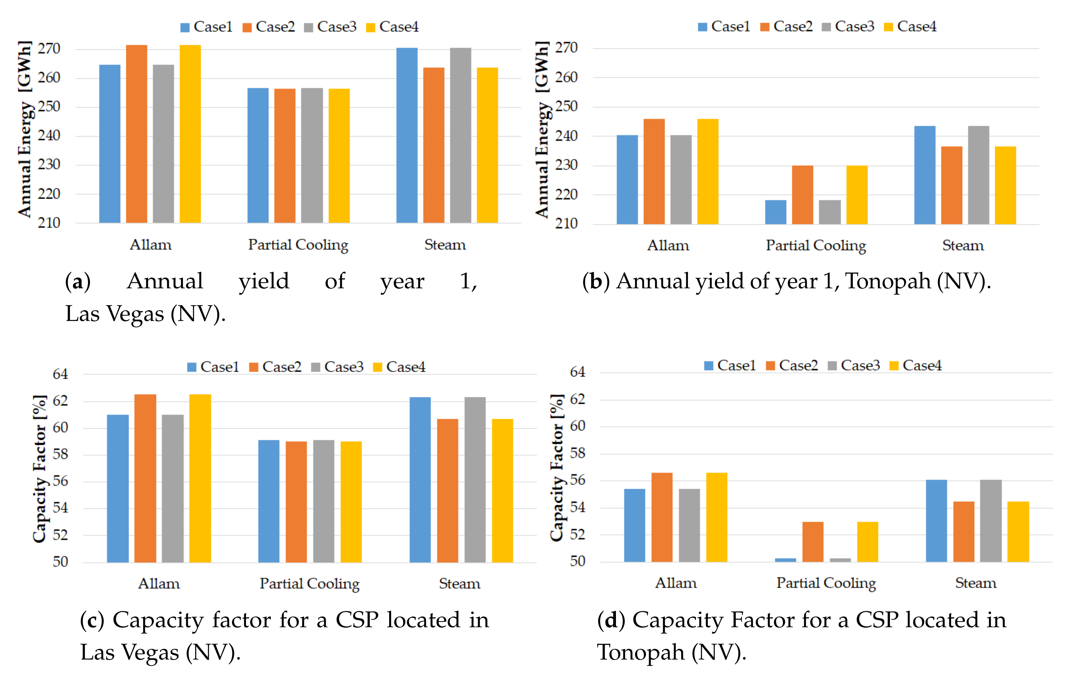
  Yield ($E_{year}$), [GWh]: this is the annual production of electricity of the power plant.

  -

  Capacity Factor ($CF$), [%]: ratio from the system’s annual production of electricity in the first year of operation to the theoretical energy production, should the system run at the rated capacity throughout the entire year. This is a measure of the electricity that the system would be able to produce if it were operated at its nominal capacity for every hour of the year, and it can be significantly affected by the plant location and by the operation (dispatch control) of the Thermal Energy Storage system.

• Financial:

  -

  Levelised Cost of Electricity $LCoE$ [¢/kWh]: a measure of the total project life cycle costs relative to the total production of energy throughout the entire project lifetime.

  -

  Net Present Value $NPV$ [$]: discounted (present) value of the net cash inflow.

  -

  Internal Rate of Return $IRR$, [%]: the nominal discount rate that would yield null $NPV$ for given economic and financial assumptions (including the sales price of electricity specified in the Power Purchase Agreement—$PPA$.

Several observations are worthwhile in Figure 7. The location of a CSP plant is expected to have a very strong impact on the annual yield. This is to be expected and is confirmed here by the larger production of electricity of the plant in Las Vegas.

Another interesting aspect, which is not as evident, is the impact of the dispatch control scheme, which yields a very variable plant performance pattern. For supercritical Carbon Dioxide plants based on the Allam cycle, the dispatch control proposed in SAM by default (Cases 1 and 3) is able to produce 5 GWh/year more energy than that proposed in the SunShot Vision Study. In order to find the reasons for this, it is reminded that the latter scheme was based on lower power settings to extend the operating time of the plant in periods with expectedly low solar availability, as opposed to the scheme proposed by SAM where power generation is maximised regardless of a potentially higher number of start-ups. The superior performance of this approach will have to be compared against the economic impact of the latter on maintenance costs in an actual power plant. Alas, as expected, the higher yield of Cases 1 and 3 in both locations translate into higher capacity factors.

Interestingly, the impact of dispatch control on plant performance for a conventional CSP plant based on a steam cycle is exactly the opposite. The dispatch control proposed in the SunShot Vision Study produces a higher yield than the default control proposed by SAM. The margin between the two is again in the order of 5 GWh/year, and the reasons for this are found in the off-design performance of the steam cycle, and to make it even more interesting, for a CSP plant using sCO${}_2$ technology based on the Partial Cooling cycle, the annual production of electricity seems to be totally insensitive to the dispatchability scheme adopted, as shown in Figure 7. The patterns discussed are applicable to both locations, which supports their dependence on the characteristics of the power block and not on the boundary conditions of the power block. All this opens a very interesting research pathway incorporating the combined optimisation of both cycle technology, cycle layout and dispatch control scheme.

From a quantitative standpoint, the foregoing qualitative considerations translate as follows, for the cases considered. A CSP plant based on the Allam cycle in Las Vegas achieves 10% higher yield and capacity factor than if it were located in Tonopah and the difference would increase to about 12.5% if a Partial Cooling sCO${}_2$ or a steam cycle were used. Regarding dispatch control, the SunShot Vision Study setting yields 3% higher $E_{year}$ and $CF$ when using the Allam cycle whereas a 3% drop in these parameters must be expected when considering a steam-turbine CSP plant. Further to the discussion in the previous paragraph, this can also be explained by the fact that SAM’s Default and SunShot Vision Study’s dispatch control modes are specifically designed for steam and sCO${}_2$ power cycles respectively.

The same capacity to significantly change the results is not observed when assessing the two sets of financial assumptions. The input parameters considered in the SunShot Vision Study always lead to better financial results than SAM’s, yielding higher $NPV$ and lower $LCoE$ for a given location, as shown in Figure 8. This is mostly due to the longer lifetime and higher IRR considered, even if the former model presents a larger debt fraction, set to 60% (versus 50% for SAM’s default case) of the total capital cost. It is also observed that $NPV$ depends on the financial model given the minor deviations seen between different locations, cycles or dispatch control systems. On the other hand, $LCoE$ happens to be strongly affected by all the factors considered so far. In particular:

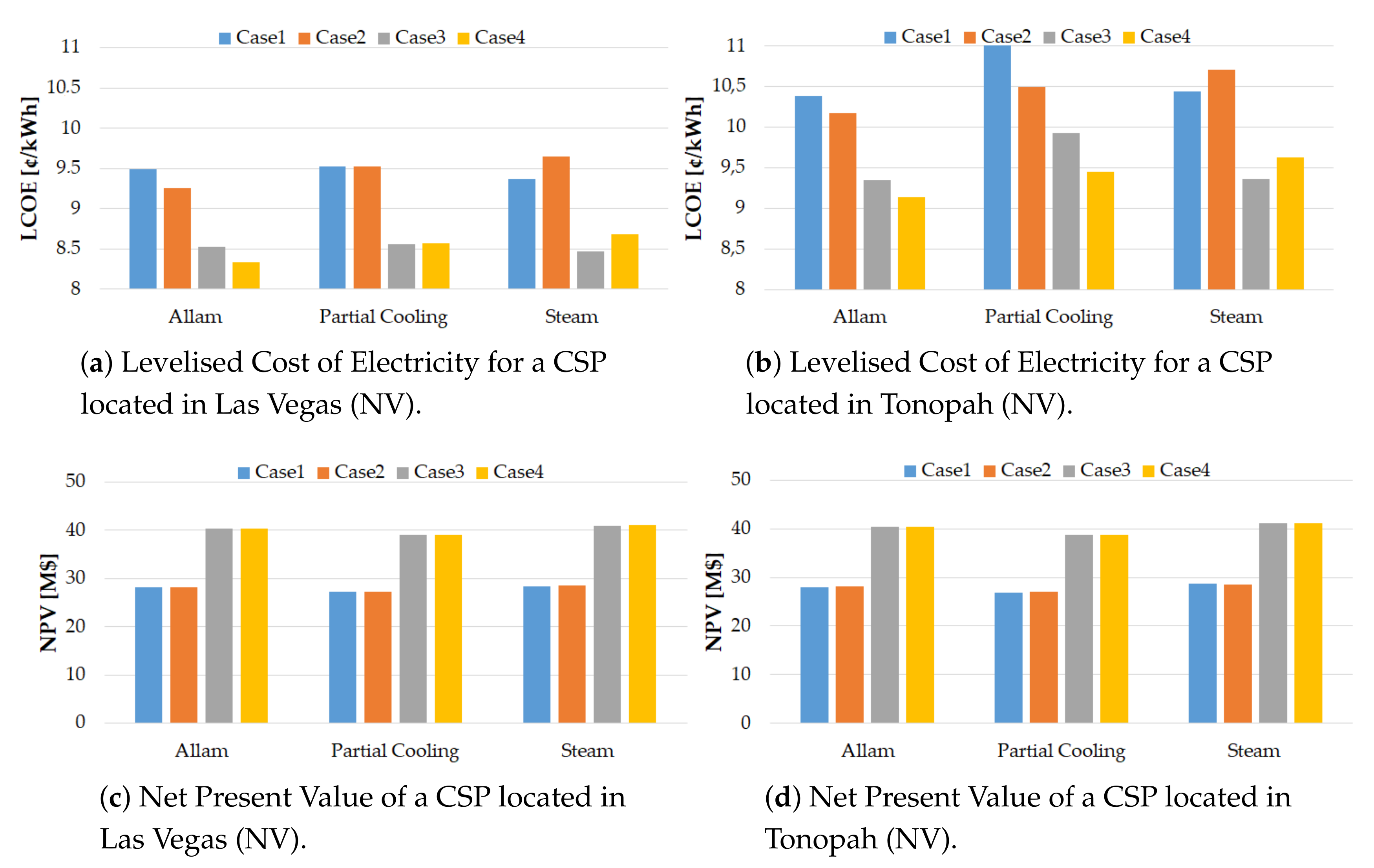
• Las Vegas yields lower $LCoE$, even if some $LCoE$s obtained with the SunShot Vision Study case considering the Allam cycle in Tonopah are comparable to those obtained by the SAM setting in Las Vegas, regardless of the cycle used.
• The trend followed by $LCoE$ is approximately symmetrical to the figures of merit indexing thermal performance ($CF$ and $E_{year}$) and balanced by the financial model. Higher $CF$ usually comes with lower $LCoE$ but, if the two options with the lowest $CF$ are considered—Partial Cooling cycle located in Tonopah for Cases 1 and 2—it is found that Case 1 always yields the highest $LCoE$ whereas the SunShot model can compensate for the $CF$ effect in Case 3.
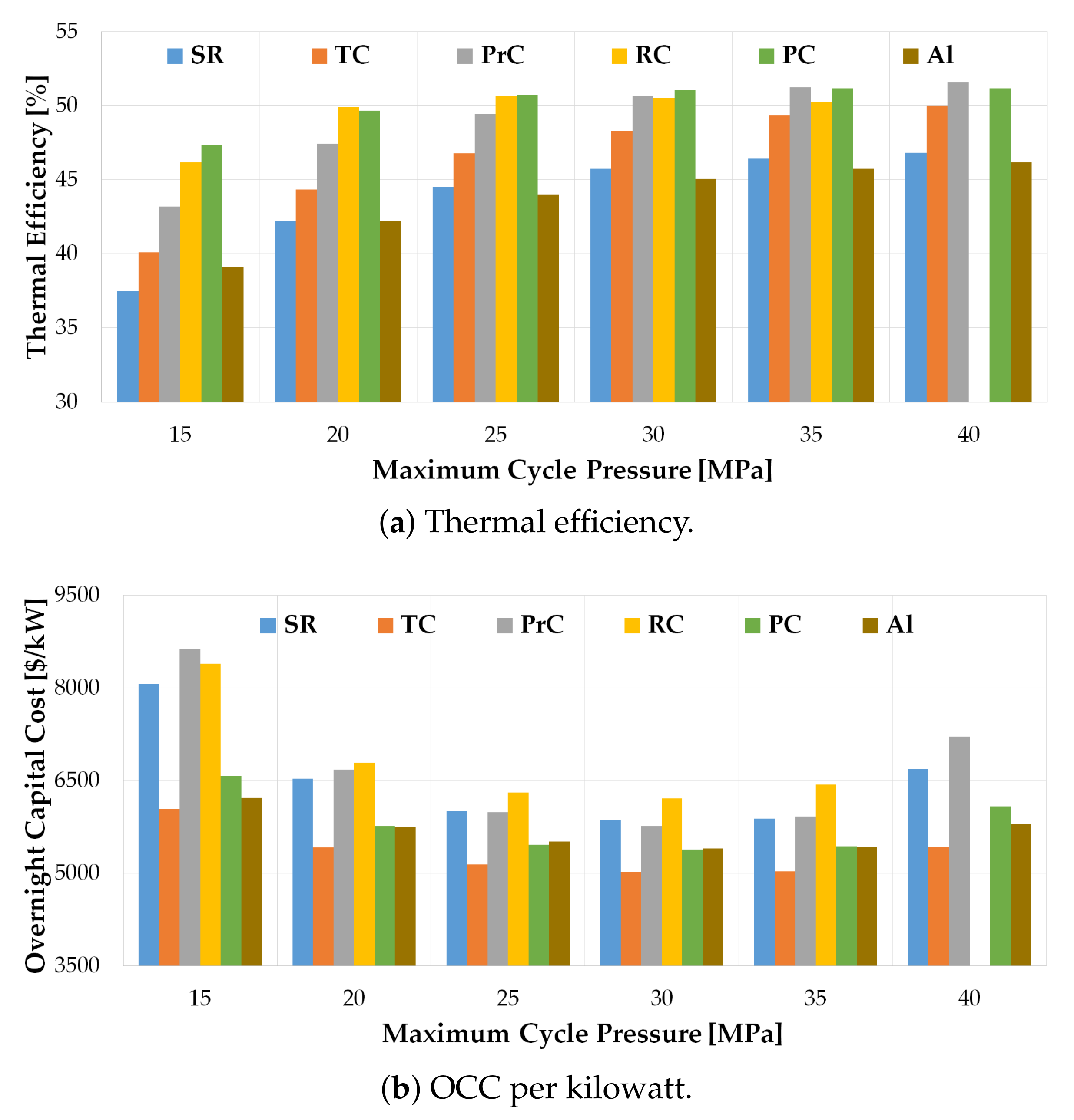
• If the same financial model is considered (Cases 1–2, Cases 3-4), the lowest $LCoE$s are achieved by plants presenting better performance metrics (higher $CF$ and $E_{year}$), as observed in Figure 7a,b and Figure 8a,b. Based on this foreseeable result, increasing the capacity factor of a plant (and therefore its annual yield) is confirmed to be of capital importance to increase the feasibility of sCO${}_2$-based CSP plants.

Based on the foregoing results, it is difficult to ascertain the best power cycle, given that the three power cycles yield very similar $LCoE$ in the order of 8.5–9.5 ¢/kWh, see Figure 8a,b. Moreover, the small differences observed lie within the cumulative uncertainty incurred by all the assumptions made throughout the analysis.

Figure 9 presents the final comparison of $LCoE$ for the reference plant using the power cycles considered. The length of each bar comes determined by the values taken by $LCoE$ for the different cases considered in Table 6. The lowest cost of electricity is obtained for the best combination of the Allam cycle (8.33 ¢/kWh), while the worst case based on the Partial Cooling cycle yields the highest $LCoE$ (11.02 ¢/kWh). Interestingly, the range of $LCoE$ for plants based on steam turbine technology falls entirely within the values covered by the other cycles. This confirms the lack of a clear, unambiguous conclusion about the optimum CSP plant concept stemming from this work, as suggested in the introductory section of the paper. To the authors’ opinion, however, this result does confirm the large potential of sCO${}_2$ power cycles for CSP applications, which must be considered as a solid alternative to the standard steam Rankine cycle approach in spite of the apparently marginal gain suggested by Figure 9. Such a strong statement is based on the fact that, even if the results obtained are still far from the 6 ¢/kWh target set by the SunShot programme (or 3 ¢/kWh in the longer term), it must not be forgotten that the $LCoE$ values presented in this paper for sCO${}_2$ are estimates based on deliberately conservative assumptions. For instance, the utilisation of molten salts that are less costly than FLiNaK, which is a reasonable assumption for an actual power plant in the future, would certainly cut down installation costs and, therefore, $LCoE$ by a large fraction given the dominant role of the Thermal Energy Storage System in determining the economic performance of the plant. This is a very likely possibility in the near future which would cut LCoE down for the sCO${}_2$ cases in Figure 9 but would not affect the cost of the steam-based case. Therefore, it may as well be the case that mid-term CSP plants employing Allam and Partial Cooling cycles are able to achieve $LCoE$s lower than those obtained in this research, and closer to the SunShot objective, once the very strong economies of scale that are characteristic of CSP start impacting sCO${}_2$ power blocks. There is no reason why a cost decline similar to that experienced by conventional CSP-STE plants cannot be experienced by this new technology in the near term.

Figure 9. Range of Levelised Cost of Energy ($LCoE$) for CSP plants based on different power cycles.

With this in mind, it is concluded that more accurate part-load models and integration schemes in SAM or equivalent software will prove that either the Allam or Partial Cooling cycle layouts have the potential to make a strong case for the next generation of CSP plants based on sCO${}_2$ power cycles, enabling the ambitious objectives targeted by the SunShot Program. In this regard, it is interesting to see how the selection of a particular set of assumptions (both financial, economic and thermal) has the potential to turn the Recompression cycle into a competitive option to achieve the 6 ¢/kWh target of the SunShot programme [28], which is certainly in contrast with the conclusions obtained in this work. Far from discussing the credibility of other research works, the latter statement aims to highlight that much more work on the assessment of appropriate sets of non-technical boundary conditions is still required.

4. Some Considerations about Uncertainty

Assessing a trustworthy and thorough feasibility analysis of CSP plants employing sCO${}_2$ power blocks is very challenging, mostly due to the low TRL and MRL of sCO${}_2$ technology and to the scarcity of reliable cost-related information. To overcome this limitation, this work is based on a series of assumptions, in order to reduce the complexity of the problem down to a manageable level. In this section, these assumptions are revisited with the aim to assess the reliability of the results, highlighting both the positive features and also the main flaws.

There are two types of uncertainty when exploring the potential of disruptive technologies: avoidable and unavoidable. Avoidable uncertainty that is incurred in the simulation of processes due to the lack of precise information about the operating conditions and specifications of certain components. The same applies to the calculation of capital and operating costs of a technology that is not commercially available yet. As far as this work is concerned, previous publications by the authors have justified the simplifying assumptions made to carry out the thermal assessment [8,11] and to estimate the capital costs of sCO${}_2$ technology [9,10]. In this former case, the performance results have been validated against results in literature and also against experimental data [30]. For capital costs, given the lack of mass production of the equipment needed (sCO${}_2$ compressors, expanders and heat exchangers and also high pressure and temperature solar receivers), a dedicated Monte Carlo- based uncertainty quantification analysis is incorporated in the calculations. In either case, uncertainty can be classified as avoidable inasmuch as the continuous development of the technology and, later, the deployment of a commercial plant will expectedly yield more accurate technical and economic information.

The financial boundary conditions set to calculate the Levelised Cost of Electricity of the technology is affected by the so-called unavoidable uncertainty. Future economic scenarios are not foreseeable and, more often than not, previsions are drastically altered by unpredictable political and/or social changes; the twenty-first century is still in its infancy and it has already seen several of these crises. As a consequence of this, setting the discount rate turns out an uncertain process that includes thorough considerations about how investments in a particular market might unfold in the future. The same applies to other local assumptions related to foreseen energy policies and subsidies, especially in unstable regions of the world [31]. These aspects involved in the economic valuation of constructing innovative CSP plants are inherently uncertain and, therefore, cannot be removed from the analysis completely.

With all this in mind, the results obtained are deemed as trustworthy as possible for a technology that is still far from the marketplace. Moreover, as reported in the concluding remark of the previous section, the results obtained are thought to provide a very solid upper limit of the expected $LCoE$ enabled by sCO${}_2$ power cycles in CSP applications. From here, future works will continuously reduce avoidable uncertainty to values comparable to those reported for state-of-the-art CSP plants based on steam turbines.

5. Conclusions

This paper is focused on the assessment of the Levelised Costs of Electricity that should be expected if supercritical CO${}_2$ power cycles were adopted in next generation Concentrated Solar Power plants for Solar Thermal Electricity generation. A simulation platform developed by the authors for the techno-economic analysis of Concentrated Solar Power plants has been integrated with the Solar Advisor Model to produce a larger simulation tool enabling the assessment of technical and non-technical plant characteristics to a level of detail not enabled by the latter software alone.

Plants based on steam turbine technology and on sCO${}_2$ cycles have been analysed under different financial/economic boundary conditions and for two different locations which can be regarded as above-average for CSP installations. In all cases, the net output of the plant is 50 MW and the Thermal Energy Storage system is sized to enable operation at full capacity for ten hours. In the most favourable cases, the Partial Cooling and Allam cycles provide an $LCoE$ of 8.56 ¢/kWh and 8.33 ¢/kWh respectively, along with a Capacity Factor of around 59% and 62.5%. On the contrary, in the worst case, the $LCoE$ of the Partial Cooling cycle increases to 11 ¢/kWh, with a $CF$ slightly higher than 50%, while the values of the Allam cycle are 10.38 ¢/kWh and 55.4% respectively.

When these figures of merit are compared with a reference plant based on a state-of-the-art steam Rankine cycle, the main finding is that both sCO${}_2$ cycles have the potential to yield $LCoE$s comparable to those of the reference plant, or even lower. Taking into account the conservative approach employed throughout the present work, especially in terms of installation costs, this comes to confirm that sCO${}_2$ power cycles are an interesting alternative to enhance the competitiveness of CSP-STE plants in the mid to long term, even if the drastic cost reductions claimed by some authors seem not to be so straightforward in the short term. In the longer term, mass deployment and a further refinement of the technology (technology/cost-wise) will very likely increase the economic gains of CSP-sCO${}_2$ plants but, at the moment, this remains yet to be verified.

In this regard, it is worth highlighting the groundbreaking concept proposed by the SCARABEUS project, funded by the European Commission and running from 2019 to 2023. In this project, CO${}_2$ is doped with certain compounds to modify the critical properties of the resulting mixture, shifting the critical temperature to higher values and enabling the practical implementation of condensing sCO${}_2$ cycles (for instance, the Transcritical CO${}_2$ cycle would be realisable even at very high ambient temperatures). Substituting these new CO${}_2$ mixtures for pure CO${}_2$ in the same layouts would, in turn, boost the efficiency of the resulting power plant, which translates into a smaller footprint of the solar field and also smaller size of the Thermal Energy Storage system. If these were eventually possible, as already suggested by the preliminary results in [3], the resulting power plant would easily reduce the LCoE reported in this paper by a large margin, possibly achieving the ambitious targets set forth by the SunShot programme.

References

- Office of Energy Efficiency & Renewable Energy—The Sunshot Iniciative. Available online: https://www.energy.gov/eere/solar/sunshot-initiative (accessed on 15 March 2019).
- Manzolini, G.; Binotti, M.; Bonalumi, D.; Invernizzi, C.; Iora, P. CO2 mixtures as innovative working fluid in power cycles applied to solar plants. Techno-economic assessment. Solar Energy 2019, 181, 530–544. [Google Scholar] [CrossRef]
- Binotti, M.; Di Marcoberardino, G.; Iora, P.; Invernizzi, C.M.; Manzolini, G. Supercritical carbon dioxide/alternative fluids blends for efficiency upgrade of solar power plant. In Proceedings of the 3rd European Conference on Supercritical CO2 (sCO2) Power Systems 2019, Paris, France, 19–20 September 2019; pp. 222–229. [Google Scholar]
- Crespi, F.; Gavagnin, G.; Sánchez, D.; Martínez, G. Supercritical Carbon Dioxide Cycles for Power Generation: A Review. Appl. Energy 2017, 195, 152–183. [Google Scholar] [CrossRef]
- Sulzer, G. Verfahren zur Erzeugung von Arbeit aus Warme. Swiss Patent 269599, 15 July 1950. [Google Scholar]
- Angelino, G. Carbon Dioxide Condensation Cycles for Power Production. J. Eng. Power 1968, 90, 287–295. [Google Scholar] [CrossRef]
- Feher, E. The supercritical thermodynamic power cycle. Energy Conv. Manag. 1968, 8, 85–90. [Google Scholar] [CrossRef]
- Crespi, F.; Gavagnin, G.; Sánchez, D.; Martínez, G. Analysis of the Thermodynamic Potential of Supercritical Carbon Dioxide Cycles: A Systematic Approach. J. Eng. Gas Turb. Power 2017, 140, 051701. [Google Scholar] [CrossRef]
- Crespi, F.; Sánchez, D.; Rodríguez, J.; Gavagnin, G. Fundamental Thermo-Economic Approach to Selecting sCO2 Power Cycles for CSP Applications. Energy Procedia 2017, 129, 963–970. [Google Scholar] [CrossRef]
- Crespi, F.; Sánchez, D.; Sánchez, T.; Martínez, G.S. Capital Cost Assessment of Concentrated Solar Power Plants Based on Supercritical Carbon Dioxide Power Cycles. J. Eng. Gas Turb. Power 2019, 141, 071011. [Google Scholar] [CrossRef]
- Crespi, F.; Sánchez, D.; Sánchez-Lencero, T.; Martínez, G.; Muñoz, A. Off-design operation of Supercritical Carbon Dioxide Power Cycles in Concentrated Solar Power plants. Appl. Thermal Eng. 2020, in press. [Google Scholar]
- SCARABEUS. D5.1 Report on Best Available Technologies (BAT) for Central Receiver Systems; Technical Report; Abengoa Energia, University of Seville: Seville, Spain, 2019. [Google Scholar]
- Martin, M. Techno-Economic Assessment of Concentrated Solar Power Tower Plants Integrating Pressurised Air Rceivers and Gas Turbines. Ph.D. Thesis, University of Seville, Seville, Spain, 2018. (In Spanish). [Google Scholar]
- Williams, D. Assessment of Candidate Molten Salt Coolants for the NGNP/NHI Heat-Transfer Loop; Technical Report; Oak Ridge National Lab (ORNL): Oak Ridge, TN, USA, 2006.
- Mehos, M.; Turchi, C.; Vidal, J.; Wagner, M.; Ma, Z.; Ho, C.; Kolb, W.; Andraka, C.; Kruizenga, A. Concentrating Solar Power Gen3 Demonstration Roadmap; Technical Report; National Renewable Energy Lab (NREL): Golden, CO, USA, 2017.
- Yoon, S.; Sabharwall, P.; Kim, E. Analytical Study on Thermal and Mechanical Design of Printed Circuit Heat Exchanger; Technical Report; Idaho National Laboratory: Idaho Falls, ID, USA, 2013.
- Prieto, C.; Fereres, S.; Ruiz-Cabañas, F.J.; Rodriguez-Sanchez, A.; Montero, C. Carbonate molten salt solar thermal pilot facility: Plant design, commissioning and operation up to 700 °C. Renew. Energy 2020, 151, 528–541. [Google Scholar] [CrossRef]
- Turchi, C.S.; Ma, Z.; Neises, T.W.; Wagner, M.J. Thermodynamic study of advanced supercritical carbon dioxide power cycles for concentrating solar power systems. J. Solar Energy Eng. 2013, 135, 041007. [Google Scholar]
- Dyreby, J.; Klein, S.; Nellis, G.; Reindl, D. Design considerations for supercritical carbon dioxide Brayton cycles with recompression. J. Eng. Gas Turb. Power 2014, 136, 101701. [Google Scholar] [CrossRef]
- Silvestri, G. Eddystone Station, 325 MW Generating Unit, A Brief History; ASME: Philadelphia, PA, USA, 2003. [Google Scholar]
- Weiland, N.T.; Lance, B.W.; Pidaparti, S.R. sCO2 Power Cycle Component Cost Correlations From DOE Data Spanning Multiple Scales and Applications. In Proceedings of the ASME Turbo Expo 2019: Turbomachinery Technical Conference and Exposition, Phoenix, AZ, USA, 17–21 June 2019. [Google Scholar]
- Carlson, M.D.; Middleton, B.M.; Ho, C.K. Techno-economic comparison of solar-driven SCO2 Brayton cycles using component cost models baselined with vendor data and estimates. In Proceedings of the ASME 2017—11th International Conference on Energy Sustainability Collocated with the ASME 2017 Power Conference Joint With ICOPE-17, the ASME 2017 15th International Conference on Fuel Cell Science, Engineering and Technology, and the ASME 2017 Nuclear Forum (Digital Collection); American Society of Mechanical Engineers (ASME): New York, NY, USA, 2017. [Google Scholar]
- IRENA. Renewable Power Generation Costs in 2018; International Renewable Energy Agency: Abu Dhabi, UAE, 2019. [Google Scholar]
- Allam, R.; Fetvedt, J.; Forrest, B.; Freed, D. The Oxy-Fuel, Supercritical CO2 Allam Cycle: New Cycle Developments to Produce Even Lower-Cost Electricity From Fossil Fuels Without Atmospheric Emissions. In Proceedings of the ASME Turbo Expo 2014: Turbine Technical Conference and Exposition, Düsseldorf, Germany, 16–20 June 2014. [Google Scholar]
- Kulhánek, M.; Dostal, V. Thermodynamic analysis and comparison of supercritical carbon dioxide cycles. In Proceedings of the Supercritical CO2 Power Cycle Symposium, Boulder, CO, USA, 24–25 May 2011; pp. 1–7. [Google Scholar]
- Neises, T.; Turchi, C. Supercritical CO2 Power Cycles: Design Considerations for Concentrating Solar Power. In Proceedings of the 4th Supercritical CO2 Power Cycles Symposium, Pittsburgh, PA, USA, 9–10 September 2014; Volume 2, pp. 9–10. [Google Scholar]
- Crespi, F. Thermo-Economic Assessment of Supercritical CO2 Power Cycles for Concentrated Solar Power Plants. Ph.D. Thesis, Unviersity of Seville, Seville, Spain, 2019. [Google Scholar]
- Schmitt, J.; Wilkes, J.; Allison, T.; Bennett, J.; Wygant, K.; Pelton, R. Lowering the Levelized Cost of Electricity of a Concentrating Solar Power Tower With a Supercritical Carbon Dioxide Power Cycle. In Proceedings of the ASME Turbo Expo 2017: Turbomachinery Technical Conference and Exposition (Digital Collection), Charlotte, NC, USA, 26–30 June 2017. [Google Scholar]
- Ho, C.; Mehos, M.; Turchi, C.; Wagner, M. Probabilistic Analysis of Power Tower Systems to Achieve Sunshot Goals. Energy Procedia 2014, 49, 1410–1419. [Google Scholar] [CrossRef][Green Version]
- Crespi, F.; Sánchez, D.; Hoopes, K.; Choi, B.; Kuek, N. The Conductance Ratio Method for Off-Design Heat Exchanger Modeling and its Impact on an sCO2 Recompression Cycle. In Proceedings of the ASME Turbo Expo 2017: Turbomachinery Technical Conference and Exposition (Digital Collection), Charlotte, NC, USA, 26–30 June 2017. [Google Scholar]
- Sánchez, D.; Bortkiewicz, A.; Rodr’íguez, J.; Martínez, G.; Gavagnin, G.; Sánchez, T. A methodology to identify potential markets for small-scale solar thermal power generators. Appl. Energy 2016, 169, 287–300. [Google Scholar] [CrossRef]