On the Procedure of Draught Rate Assessment in Indoor Spaces

Featured Application

In case the ventilation system design leads to low-frequency high-amplitude air velocity pulsations, strong time variation of the draught rate (DR) index may exist and the thermal environment categorization requires for space-distributed long-term computations and measurements.

Abstract

The objective of the paper is to demonstrate the importance of the unsteady Computational Fluid Dynamics (CFD) simulations and long-term measurements for the reliable assessment of thermal comfort indoors, for proper categorization of the indoor thermal environment and for identifying the reasons for complaints due to draught discomfort. Numerical simulations and experimental measurements were applied in combination to study ventilation in a field laboratory, a university classroom with a controlled indoor environment. Strong unsteadiness of the airflow was registered both in the unsteady RANS results and the real-scale long-term velocity data measured with thermo anemometer. Low-frequency high-amplitude velocity fluctuations observed lead to substantial time variation of the draught rate. In case of categorization of a thermal environment, the point measurements or steady-state RANS computations would lead to wrong conclusions as well as they cannot be used for identification of the reasons for people’s complaints due to draught discomfort if strong unsteadiness of the airflow exists. It is demonstrated that the length of the time interval for draught rate (DR) assessment may not be universal if low-frequency high-amplitude pulsations are present in the room airflow.

1. Introduction

The indoor environmental quality (IEQ) depends on both indoor air quality (IAQ) and human comfort (thermal, visual, acoustic). A poor IEQ could precondition different discomforts and health problems that result in short or and long-term absence from work and decreased productivity [1,2,3].

Olesen et al. [4] reported that in more than 40% of enclosures people complain from the comfort or health-related issues. The situation is worsening in schools, where the occupation density is 1.8–2.4 m²/person, compared to 10 m²/person in offices [5]. Improving the working environment and related costs can be offset by better productivity [6] and overall comfort [7]. There is a need for studies on the assessment of ventilation strategies in terms of their efficiency while aiming to provide the comfort of the occupants [8,9,10].

According to ISO 7730:2005 [11], the thermal environment in an indoor space can be assessed in 3 categories. Two factors determine each category: the thermal state of the body, evaluated by the Predicted percentage of dissatisfied (PPD) index, and the local discomfort. One of the indices for local discomfort is the draught rate (DR). The achievement of air distribution without draught is one of the goals of the ventilation methods for indoor spaces. The high air velocity in the occupied zone could be easily perceived as draught that provokes thermal comfort dissatisfaction and complaints.

Various studies assessed DR as a part of the evaluation of the thermal environment. Gendelis et al. [12] investigated test buildings with a variety of wall envelops and different heating/cooling systems. They calculated the local discomfort due to DR for 2-hour periods and the value of 40% for local turbulence intensity. Simone et al. [13] determined DR and thermal asymmetry as the most important factors for complaints among the cashiers in the studied supermarket. However, the study could not prove the statistical significance of DR on the overall thermal sensation of the occupants.

Mumovic et al. [14] investigated the winter IAQ and thermal comfort in new secondary schools, applying ISO 7730:2005 [11]. They have found out that both mechanical and hybrid ventilation systems caused problems with draughts (the draught risk exceeded 15%). On this basis, the authors suggested a more careful design of the ventilation systems in classrooms. Recently, Kiil et al. [15] reported their assessment of the draught and thermal comfort in an office building. It was found that DR was below 10% in heating and transient period measurements, but the risk of draught was assessed for the intensive cooling mode. In a later paper [16], it was concluded that avoiding fan coil units for cooling would not guarantee better thermal comfort for the occupants without draught complaints.

Numerical studies that involved DR assessment were also performed. Koper et al. [17] used numerical predictions to evaluate the thermal comfort of people in an indoor swimming pool. Though it was concluded that in a significant part of the pool the thermal comfort conditions were not reached, the authors reported that there was no draught risk. Deng and Tan [18] investigated a naturally ventilated plan office, applying a numerical analysis of local thermal comfort. They reported an effect of the high outdoor wind speed and low air temperature on the increment of the indoor DR.

Several other studies [19,20,21,22,23,24] identified DR to be the main cause of thermal discomfort even in the case that other characteristics of the thermal environment have been within the standard limits. Therefore, the correct determination of DR is of crucial importance, and each case study may help to improve the knowledge of its evaluation.

The assessment of the DR is performed, following the approach of Fanger et al. [25], implemented in ISO 7730:2005 [11]. Attempts for different calculation of DR also exist, like the innovative method in [26], developed for semi-outdoor spaces. Other standards that deal with thermal comfort models used for design, assessment, and categorization of the indoor thermal environment, are ANSI/ASHRAE Standard 55-2017 [27] and EN 16798-1:2019 [28].

ISO 7730:2005 [11] defines, and EN 16798-1:2019 [28] applies four types of local discomforts: radiant asymmetry in both the horizontal (left-right, front-back) and the vertical plane (top-bottom), the vertical temperature difference between the ankle and head level, floor temperature, and DR. ANSI/ASHRAE Standard 55-2017 [27] applies only the first three discomforts. ISO 7730:2005 [11] provides models for evaluation of the percentage of dissatisfied (PD) due to each of these discomforts. The two other standards [27,28] prescribe design criteria for the indoor thermal environment and suggest some procedures for the design.

Satisfying all requirements of one of the standards during the design of the thermal environment in densely occupied spaces with total volume ventilation is a complicated task. The numerical simulations based on Computational Fluid Dynamics (CFD) are relatively easy tools for designing the thermal environment indoors [29,30,31]. Typically, RANS (Reynolds Averaged Navier-Stokes) technique combined with a turbulence model and models for evaluation of all indices characterizing the indoor thermal environment is applied [32]. There are models for all indices, except for the DR.

The prediction of DR, based on steady-state CFD simulations with applied RANS technique, is relatively easy since all needed quantities are provided by the numerical solution [33]. However, RANS results depend strongly on the particular turbulence model used. RANS uncertainties could be significant, especially when modelling is applied to a fully-developed turbulent jet in combination with a moderate Reynolds number flow in low-velocity occupied zone [34]. To get more accurate predictions of turbulent flows, an unsteady eddy-resolving technique should be applied, like Large Eddy Simulation, LES [35], implicit LES or, in case of limited computational resources, Unsteady RANS (URANS). Calculation of DR based on discrete physical measurements or unsteady CFD simulation, e.g., URANS technique, is much more complicated. DR assessment based on numerical predictions and measurements requires information for the length of the time interval, over which mean air temperature, mean air velocity, and turbulence intensity, are calculated. Information about the sampling rate (1/Δτ) is also needed. No version of [11], even the last one, has provided information for these quantities.

The reason is that the DR model was developed based on an exposure period of 15 min [25]; an analogue constant temperature thermo anemometer measured the air velocity, and the definition of a sampling rate was meaningless. A procedure for assessment of DR in practice was developed later in collaboration between the Technical University of Denmark and Technical University of Sofia research groups; this procedure was described in detail in [36]. The measuring interval and the sampling rate were set to 3 min and 5 Hz, respectively. However, these values cannot be universally applied since impulse sources (fans, fan coils) and air terminal devices (ATD) with different characteristics are used in the ventilated spaces (with different size and shape). As a result, flows characterized by a wide variety of time and length scales would exist in the particular indoor space.

Kiil et al. [16] also provided criticism towards the existing standards in terms of DR: they found out that the standards do not specify how to select relevant conditions and locations for measurement of DR. The study has also concluded that the standards do not provide questionnaires for the assessment of occupant dissatisfaction, which are detailed enough.

The objective of this paper is to initiate discussions for improvement of the ISO 7730:2005 [11] procedure for DR assessment in indoor spaces when strong unsteadiness of the airflow is expected. It does not provide the remedy but points the attention to possible problems with DR assessment in large spaces with more than one air supply opening. Numerical simulations and experimental measurements were applied in combination to study ventilation in a test university classroom with a controlled indoor environment. The paper demonstrates the importance of the unsteady computer simulations and long-term measurements for the reliable assessment of thermal comfort indoors, for proper categorization of the indoor thermal environment, and for identifying the reasons for complaints due to draught discomfort.

2. Problem Formulation

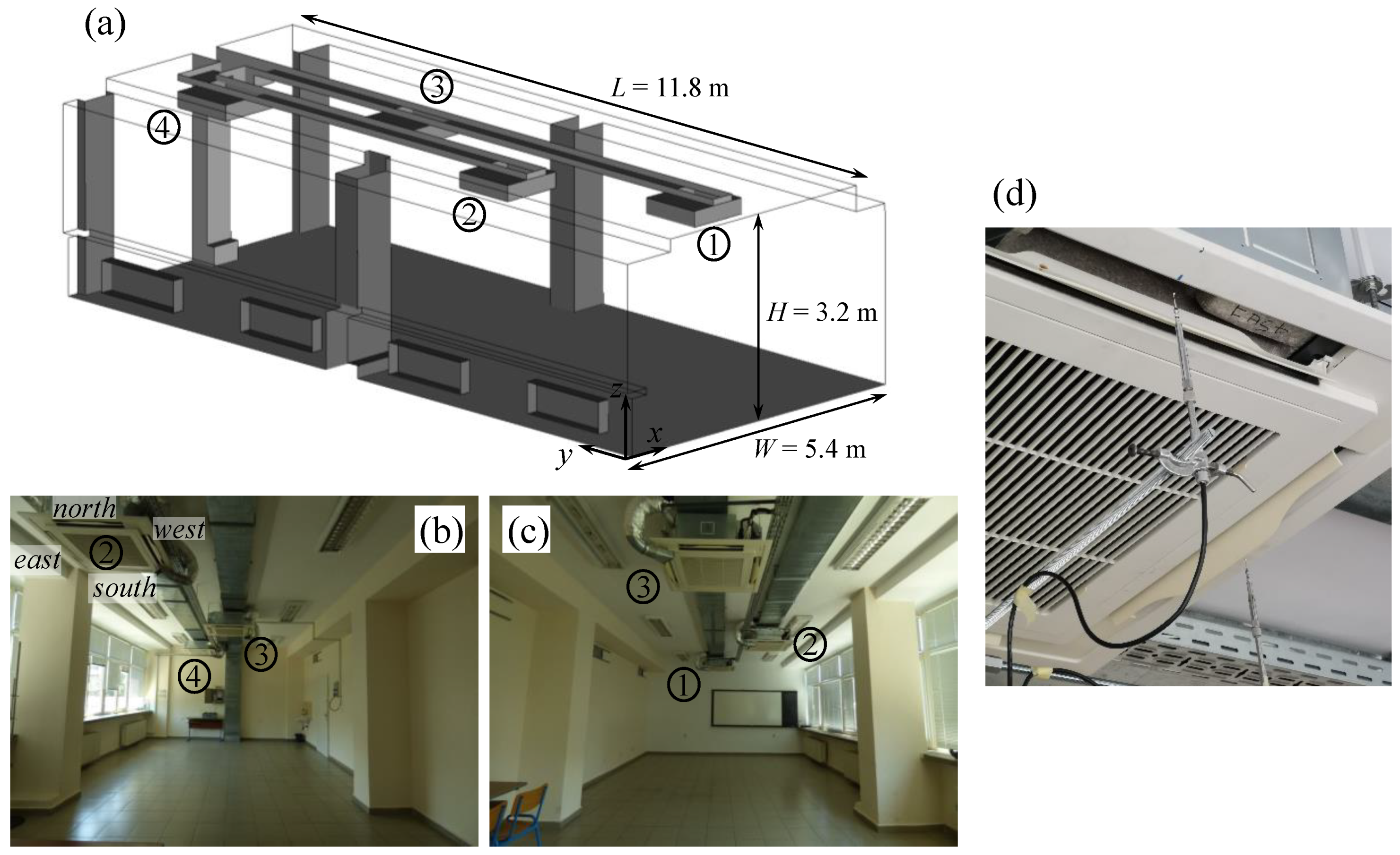
2.1. Description of the Room Geometry

The test classroom under consideration is located at the Technical University of Sofia and during the academic year it is used for teaching purposes (up to 25 persons). Figure 1 presents the geometry model built for URANS CFD calculations (Figure 1a), alongside with the classroom interior photos (Figure 1b,c) and a close-up of the fan coil (Figure 1d). In the present study, the geometry model of the room interior includes the window sill, four radiators, four columns, two ceiling beams, four ceiling diffusers (fan coils, marked as #1–4 in Figure 1a–c) and both horizontal and vertical ventilation ducts. The form of the room is a parallelepiped with the width of W = 5.4 m, the length of L = 11.8 m, and the height of H = 3.2 m. The floor area of the room is equal to W × L = 64 m² and the volume of the room is W × L × H = 204 m³. The detailed description of all room elements could be found in [37].

The air is supplied to the room by the four-way type MMU-AP0092H fan coils that could be used either in an isothermal regime or for cooling/heating purposes. Four fan coils are installed in the room in the staggered arrangement to provide various conditions for ventilation tests. The size of a fan coil is 1.0 × 1.0 × 0.25 m. It has four peripheral supply sections with the size of l_in × w_in = 0.5 × 0.07 m equipped with turning blades (louvers) and one central suction section with the size of 0.5 × 0.5 m (Figure 1b–d). The supply sections are marked as cardinal points: north, east, south, and west (Figure 1b). The louver at each supply section has five preset angles of inclination, θ, to the ceiling, namely 25°, 30°, 35°, 40°, and 45°. Figure 1d demonstrates the louver inclined at the extreme position of 45°. In the present study, two values of θ were considered, θ = 25° and θ = 45°, and it is one of the varied parameters that specifies the list of cases considered, see

Table 1. The list of cases considered.

Case	Study	θ	Cooling Mode	Time-Sample, s
#1	Experimental	25°	Nonisothermal	3600
#2	Experimental CFD	25°	Isothermal	360 7500
#3	Experimental CFD	45°	Isothermal	300, 2100 7500

. For each fan coil the fan speed could vary in the range up to 300 rpm, the maximum fan speed was set for the present experiments.

2.2. Description of Measurement Technique and Equipment

The experimental program comprised two sets of measurements. In each experiment simultaneous measurements of air velocity and air temperature at four points were performed. An 8-channel thermo anemometer composed of a multichannel power supply module SENSOR HT-430 and four thermo anemometer transducers SENSOR HT-428, each equipped with a SENSOR HT-412 (omnidirectional probe sensitive to both air velocity and air temperature) were used. The HT-412 probes meet all requirements of ISO 7726:1998 [38] standard for class C (comfort)-category desirable, i.e., accuracy better than ± (0.02 m/s + 7% of readings) and response time (90%) better than 0.2 s. The thermo anemometers were calibrated for two measurement ranges for better accuracy of the polynomial fit. The first range was between 0.03 m/s and 2.65 m/s, which corresponds to room airflow velocities. The second range was between 2 m/s and 5 m/s, which corresponds to the velocities of fan coil jets. The mean absolute error (MAE) and the normalized mean bias error (NMBE) were calculated for each sensor and both measurement ranges. The maximum sensor MAE was 0.01 m/s for measurement range 1, and 0.03 m/s for measurement range 2. It roughly corresponds to 1% normalized mean absolute error for both ranges. There was a small positive bias for the sensors in range 1 with normalized mean bias error between 0.02% and 0.05%. For range 2, the bias was practically zero with NMBE in the range ± 0.002%. The 8 voltage signals (4 proportional to air velocity and 4 proportional to air temperature) generated by the HT-412 probes were simultaneously read and stored on the hard drive of a PC by a data acquisition system manufactured by DATAQ Instruments. This system was composed of a DI-2108-P high-speed DAQ board controlled by the WinDaq recording and playback software.

The first measurement set was devoted to the characterization of airflow near the fan coil exhausts. These measurements aimed to evaluate the level of uniformity in the supply flow rates and to get data for inlet boundary conditions to be set in the CFD simulations. All fan coils were set to isothermal recirculation mode with the louver inclination of θ = 45° (case #3 in Table 1, with longer time sample). For each fan coil, the measurements of air velocity and air temperature at the middle points of four supply sections were performed simultaneously. The sensors were placed below the middle point of each opening at the distance of 0.017 m from the surface (Figure 1d). The total measuring period for each fan coil was 35 min (2100 s) long, with the sampling rate of 5 Hz. The results of this measurement set are discussed in Section 3.1.

In addition to the local measurements, at the same fan coil operation conditions the measurements of the volume flow rate Q, at each supply section of each fan coil were performed by an ALNOR Balometer.

Table 2. Air flow rate, Q, m³/h, through the supply openings of each fan coil.

Fan coil Number	East Section	South Section	West Section	North Section
#1	212	146	190	196
#2	174	158	203	191
#3	170	163	197	168
#4	164	189	193	173

summarizes the Q values.

The second set of measurements was devoted to the characterization of the airflow in the room occupied zone. Air velocity and air temperature data were collected simultaneously at four points placed one above another along a vertical line at coordinates z = 0.1 m, 0.6 m, 1.1 m, 1.7 m. According to ISO 7730:2005 [11], z = 0.1 m corresponds to the ankle level of a person, z = 0.6 m corresponds to the level of body center of gravity for a seated person, z = 1.1 m is the head level of a seated person and the body center of gravity level of a standing person, and z = 1.7 m is the head level of a standing person. The line was placed at x = 1.9 m, y = 7.4 m being the intersection of two vertical planes: the plane passing through the middle of the north supply section of fan coil #4 and the plane passing through the middle of the east supply section of fan coil #3. Monitoring points are located along this vertical line since there the supply jets from three fan coils meet – north jet of fan coil #4, the east jet of fan coil #3, and south jet of fan coil #2. The reason for selecting this vertical line is to compare velocity fluctuations parameters in the above-specified jets with the velocity fluctuation parameters in the monitoring points. Based on this a conclusion may be drawn about the reasons of velocity fluctuations at the monitoring points. Measurement point positions will be illustrated below in Section 4.1.

The measurements in the occupied zone were performed for three cases presented in Table 1. Various time intervals used for measurement data collection are given in Table 1. Both the louver inclination angle value and the fan coil operation mode varied from case to case. Isothermal recirculation mode with no outdoor air supply and no cooling/heating was provided for cases #2 and #3, while case #1 was non-isothermal. To avoid direct sunlight influence, all the measurements were done in the afternoon. However, it was not possible to keep the room temperature constant during a long measurement period. Thus, in case #1 during the whole period of 3600 s, the fan coils have been working in the cooling mode to keep an appropriate moderate temperature level in the room.

2.3. Computational Aspects

Two sets of CFD simulations of turbulent airflow in the room were performed. The aim of the first set was to reproduce the experimental conditions as much as possible. It allowed collecting the detailed data on the airflow in the room and draught rate (DR) indices. It also allowed validating the numerical data using the experimental data. The turbulent airflow in the first set of computations was modelled using the unsteady Reynolds-Averaged Navies-Stokes (URANS) approach with a fine computational grid; all geometry and boundary conditions were set as close to the experimental conditions as possible. Particular computational aspects for these CFD simulations are described in detail in Section 2.3.1.

The main goal of the second set of the CFD simulations was to demonstrate the possibilities of the up-to-date engineering CFD tools (the steady-state RANS) with a coarse computational grid to predict the DR indices. Keeping, in general, the room geometry, the problem was set with non-isothermal conditions and took into account the effects the room equipment, such as desks and chairs, as well as the occupants. Details of the problem formulation for the second set of computations are given in Section 2.3.2.

As it was mentioned in the Introduction, the RANS approach applied in the current study for turbulence modelling depends on the particular turbulence model used, and the uncertainty due to the turbulence model influence could be high. However, for multi-jet configuration considered in the study, it is not possible to use less-empirical scale-resolving simulation due to enormous computational resources required. From the literature data [39,40], it is evident that a k-ε turbulence model and the baseline SST k-ω model accurately predict jet flows and qualitatively reproduce separation zones behavior that gave a basis for the turbulence model choice in the current computations.

2.3.1. Unsteady RANS (URANS) Simulations for Computational Fluid Dynamics (CFD) Validation

Air was assumed as an incompressible fluid with constant physical properties (ρ = 1.2 kg/m³, μ = 1.8 × 10⁻⁵ kg/m⋅s). The boundary conditions at the supply sections were based on the supply flow rate values, measured in the experiments, and the effective cross-sectional area of the supply section. The mean value of volume flow rate entering the room through one supply section (averaged in time and overall 16 supply sections, Table 2) was equal to 190 m³/h (mass flow rate of 0.0647 kg/s). The area of the supply section was decreased as compared with the l_in value given in Section 2.1. The cross-section of the supply channel has smaller length then l_in (Figure 1d); the effective opening length l_{in, effective} = 0.177 m was set in the URANS computations that gave the mean inlet velocity value of U_bulk = 4.26 m/s (it corresponds to the local velocity values detected in the first set of measurements).

The uniform distribution of U_bulk was set at each supply section of each fan coil (being an inlet for the computational domain). The Reynolds number calculated using the supply section width was equal to Re = ρw_in U_bulk /μ = 2 × 10⁴. Two cases with different airflow angle values, θ = 25° and θ = 45°, were considered (they correspond to the fixed positions of the louver during the measurements, cases #2 and #3, Table 1). At the outlet boundaries (i.e., at each square suction section of each fan coil), the pressure outlet boundary condition was set assuming uniform pressure distribution. A no-slip boundary condition was set at the solid walls.

A quasi-structured grid consisted of hexahedral cells was built with the grid generator ANSYS ICEM CFD 18.2. The total cell number was 33 million cells; the cells with the smallest size were located in the corners of the inlet and outlet sections: the dimensions of these cells were 3 × 3 × 3 mm. The cells adjacent to the solid walls had the same height of 20 mm (the only exception was the solid wall at the surface of the fan coils). Depending on the local flow features, this height corresponds to the normalized distance from the center of the first near-wall cell to the wall, y⁺, in the range from the values less than one up to values exceeding 60. The sensitivity analyses of different computational parameters influence on the CFD results were performed previously and are discussed in [37]. In particular, the results of the mesh sensitivity analysis were presented in detail in [37].

The turbulence modelling of the airflow in the room was performed using the URANS approach coupled with the standard k-ε turbulence model in combination with the enhanced wall treatment. To specify the inlet boundary conditions for the turbulence characteristics the ratio of the turbulent to molecular viscosity of ν_turb/ν = 10 and the turbulent intensity of 5% were set at each supply section.

The numerical simulations were performed using the CFD package ANSYS Fluent (version 18.2) based on the finite volume method with the cell-centered variable arrangement. The iterative SIMPLEC method was used to link the continuity and momentum equations. The second-order schemes for the spatial and time discretization were chosen. The value of the time step was 0.5 s. The time step value, Δt, was varied in [37], from Δt = 0.004 s to Δt = 0.5 s, and it was found that the lower frequencies and the time-averaged flow patterns were the same in the Δt range considered. The computations were performed using the resources of Peter the Great St.Petersburg Polytechnic University Supercomputer Center (scc.spbstu.ru). In total, up to 504 cores were used for the parallel computations.

2.3.2. RANS Simulations

The steady-state RANS simulation was set for the modified geometry model, as compared with the geometry shown in Figure 1a. Namely, the ventilation ducts were removed, and the form of columns and ceiling beams was simplified. The fan coil geometry model was also modified: the fan coils were placed directly at the ceiling, and the height of each fan coil was increased to 0.3 m. The supply opening dimensions were also changed, l_in,RANS × w_in,RANS = 0.4 × 0.1 m, so that the opening area was 3.2 times larger than in URANS problem formulation. Opposite to the URANS problem formulation (and the experimental conditions) with empty room interior, the room for the RANS simulation contained 8 desks, 24 chairs, and 24 persons of simplified shape in seating positions, and one person standing upright. The detailed geometry model for this case was presented in [41].

The RANS simulation was performed for non-isothermal conditions with heat transfer problem solving. At each surface the constant values of heat flux, q, were set (

Table 3. Temperature boundary conditions for room interior elements.

Section	Wall						Seated Persons	Standing Person
	x = 0	x = 5.4 m	y = 0	y = 11.8 m	z = 0	z = 3.2 m
q, W/m2	2.32	11.67	10.15	8.04	17.52	18.23	51.41	43.50

). The mass flow inlet boundary condition was set at each supply opening, with the mass flow rate of 0.227 kg/s. This increased mass flow rate value allowed to keep almost the same value of the bulk velocity as in URANS computations, U_bulk = 5 m/s. Two cases with different air flow angle values were considered again, with the flow angle corresponded to θ = 25° and θ = 45°. It was assumed that cooled air is supplied to the room, and the constant temperature value of 17.7 °C was set at the inlets. A uniform velocity distribution, U_{bulk_out} = −0.69 m/s, was set at suction (outlet) fan coil sections. The model included also four addition outlets located at the sidewall y = 5.4 m (Figure 1b,c). They were assumed to be open, and the pressure outlet conditions were set there.

The grid used in the calculations was built in Gambit 2.4.6 grid generator. The grid consisted of cubic elements and the edge length of each cell was equal to 0.1 m. Thus, a grid suitable for engineering usage was generated, with a small number of cells (approximately 200,000). The chosen coarse grid allowed obtaining a steady-state solution due to high numerical dissipation. The problem was solved in ANSYS Fluent 6.3 using RANS approach connected with k-ω SST turbulence model. The Boussinesq approximation for buoyancy forces was used (according to the thermal balance evaluation the bulk temperature in the room was set to 24.5 °C).

3. Measurement Data

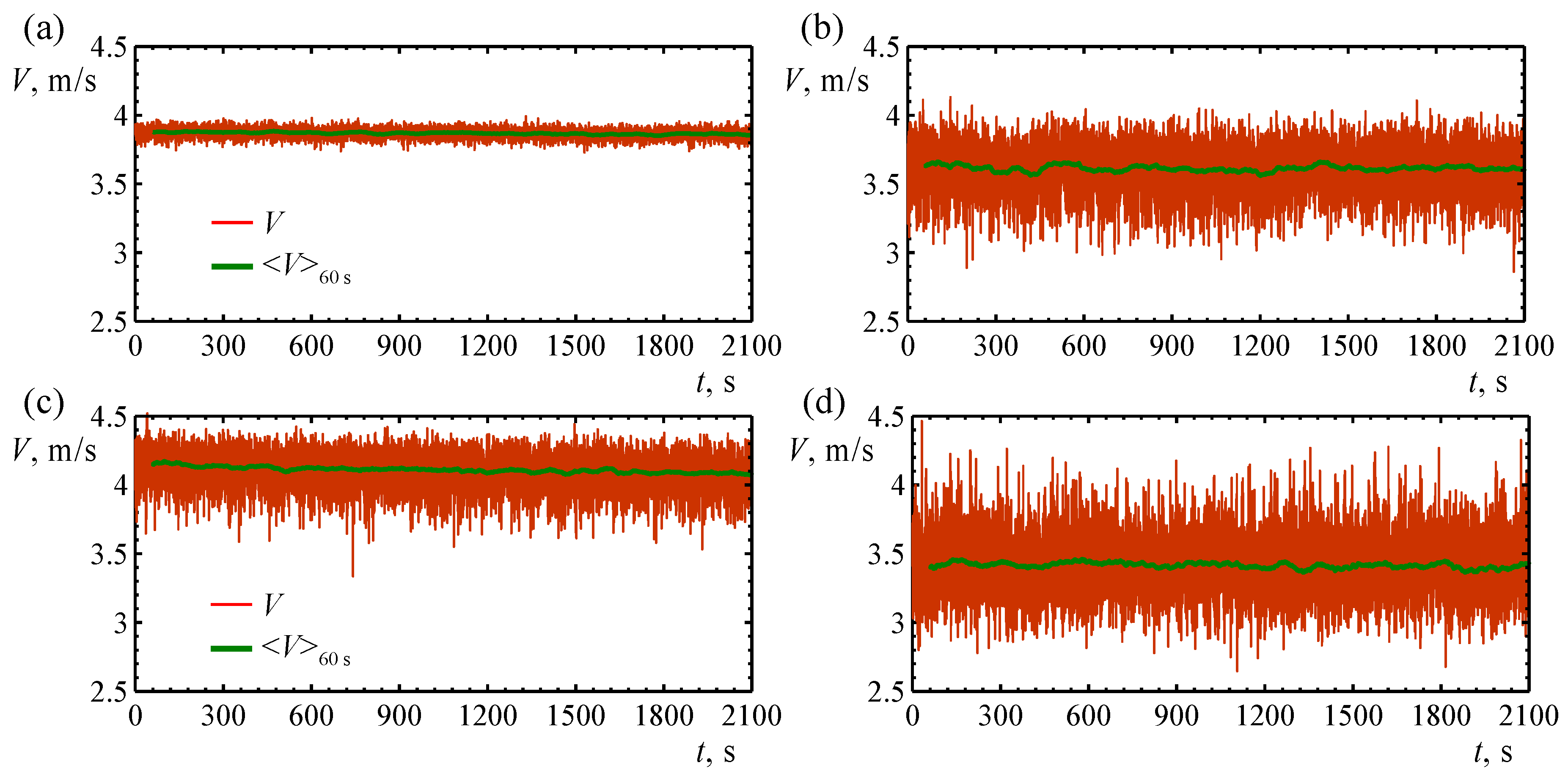
3.1. Airflow near the Fan Coil

This section presents the near fan coil velocity experimental data obtained for case #3 (Table 1) with θ = 45°. Figure 2 is an example of the velocity behavior: the data at four points located near supply sections of fan coil #4 are presented. In addition to the instantaneous velocity data (red curves), the evolution curves of the velocity time-averaged for 60 s, <V>_{60 s}, are plotted (green curves).

Table 4. Velocity characteristics at four points located near four supply sections of fan coil #4.

Supply Section	Vmin, m/s	Vaver, m/s	Vmax, m/s	Vmax − Vmin, m/s
East	3.73	3.87	3.99	0.27
South	2.86	3.61	4.13	1.27
West	3.34	4.11	4.52	1.18
North	2.65	3.42	4.46	1.82

presents the integral information on the mean velocity near the supply sections of fan coil #4 collected from the whole measurement interval of 2100 s, as well as the lowest and the highest velocity values over the measurement sample.

Table 5. Turbulent intensity at four points located near four supply sections of fan coil #4.

Outlet	<Tu>10 s, %			<Tu>30 s, %			<Tu>60 s, %
	min	mean	max	min	mean	max	min	mean	max
East	0.53	0.81	1.14	0.68	0.82	0.98	0.72	0.83	0.95
South	2.80	4.53	6.04	3.67	4.59	5.50	4.01	4.61	5.18
West	1.96	2.99	4.41	2.43	3.01	3.64	2.64	3.02	3.43
North	3.78	5.92	9.12	4.75	5.99	7.78	5.13	6.00	7.05

presents the corresponding information on the turbulence intensity: Tu = 100% [∑(V_i − <V>)²/(N − 1)]^0.5/<V>, where N is the number of measurements of instantaneous local air velocity V_i, the summation is from i = 1 to i = N. The values of Tu (Table 5) are averaged over three intervals: 10 s, 30 s, and 60 s (the variables <Tu>_{10 s}, <Tu>_{30 s}, and <Tu>_{60 s}, correspondingly).

Velocity time variation records presented in Figure 2 and the data in Table 4 clearly show that the near fan coil velocity characteristics vary much from one supply opening to another. The range of variation of air velocity at the east supply section is the smallest one (0.26 m/s) while the largest one is observed at the north supply section (1.82 m/s). Velocity variation range over the supply sections of fan coil #4 is 1.87 m/s, which is comparable with its range of variation at the north supply section. The range of variation of mean air velocity at the supply sections of fan coil #4 is 0.69 m/s. The smallest mean air velocity appears at the north supply section (3.42 m/s) and the largest one appears at the west supply section (4.11 m/s). It is evident that the pattern of the jets generated by the supply sections of fan coil #4 is different, which preconditions dissimilar interaction of the supply air jets with the room air along the direction of the jets spread.

Table 5 demonstrates that the turbulence intensity also varies significantly from one supply opening to another. Following the velocity variation data, the lowest mean <Tu>_{60 s} = 0.83% is at the east opening, where the range of variation of velocity is the smallest (0.27 m/s), while the highest mean <Tu>_{60 s} = 6.00% is at the north opening, where the range of variation of velocity is the largest (1.82 m/s). The <Tu> variation at each supply section is also pronounced. For example, at the north supply section the maximum value of <Tu>_{60 s} is 7.05%, while the minimum value of <Tu>_{60 s} is 5.13%. However, with an increase in the length of the interval for Tu assessment the range of variation of Tu at each supply section becomes narrower. Minimum Tu increases and maximum Tu decreases while the mean value increases slightly.

Various time variation patterns of both air velocity and Tu at the inspection points are due to different configuration, shape, and area of the supply channels between the fan and the supply port at the face plate of the fan coil. The measurements have shown that the other three fan coils also demonstrate noticeable variation in the supply opening velocity characteristics. This variation is in accordance with the flow rate variation visible from the data measured independently (Table 2). Both the flow rate and velocity measurements at the supply openings provided a basis for the CFD problems boundary conditions setting. It could be concluded, however, that the uniform velocity and turbulence intensity distribution adopted in the computations could be treated as the first approach only.

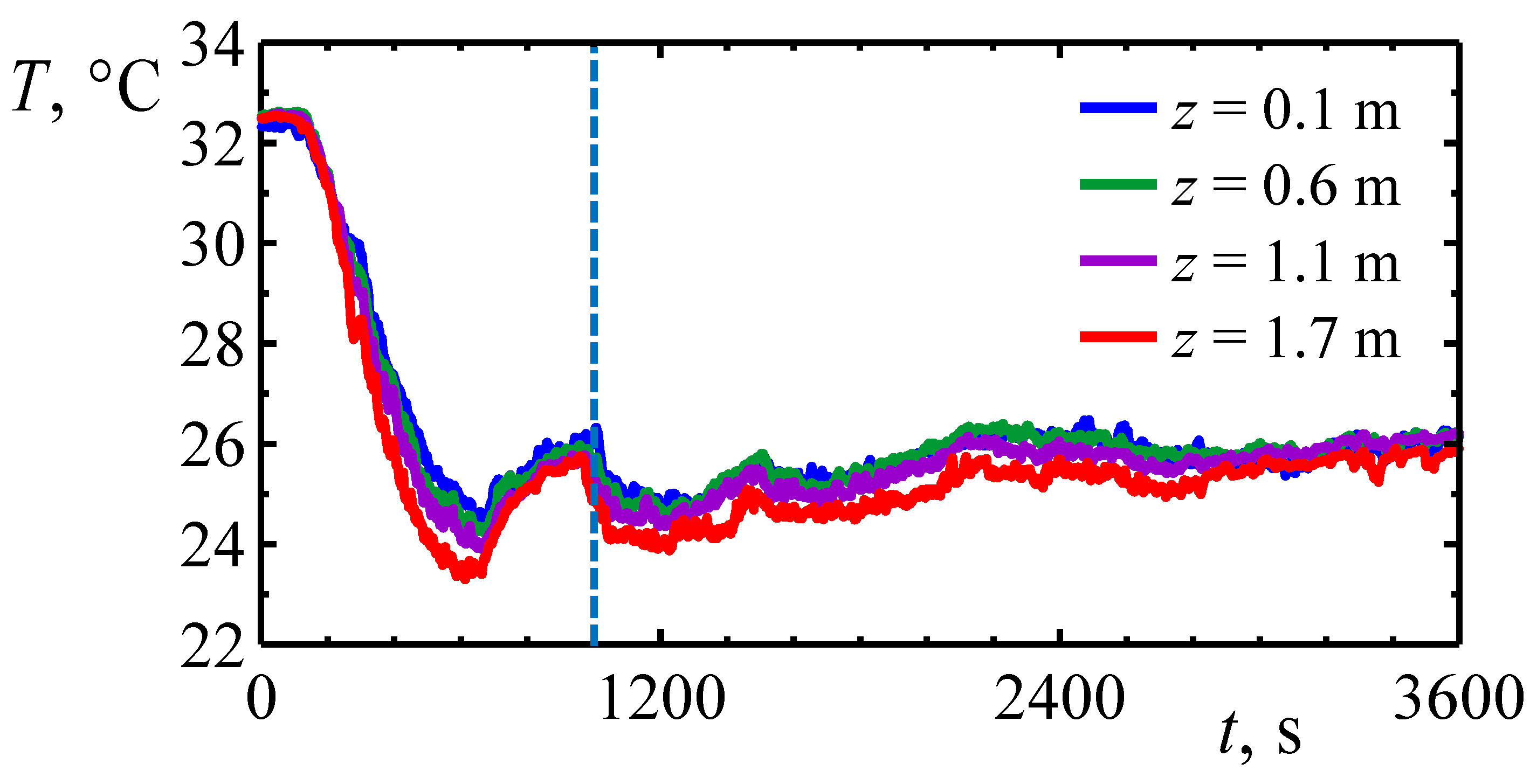
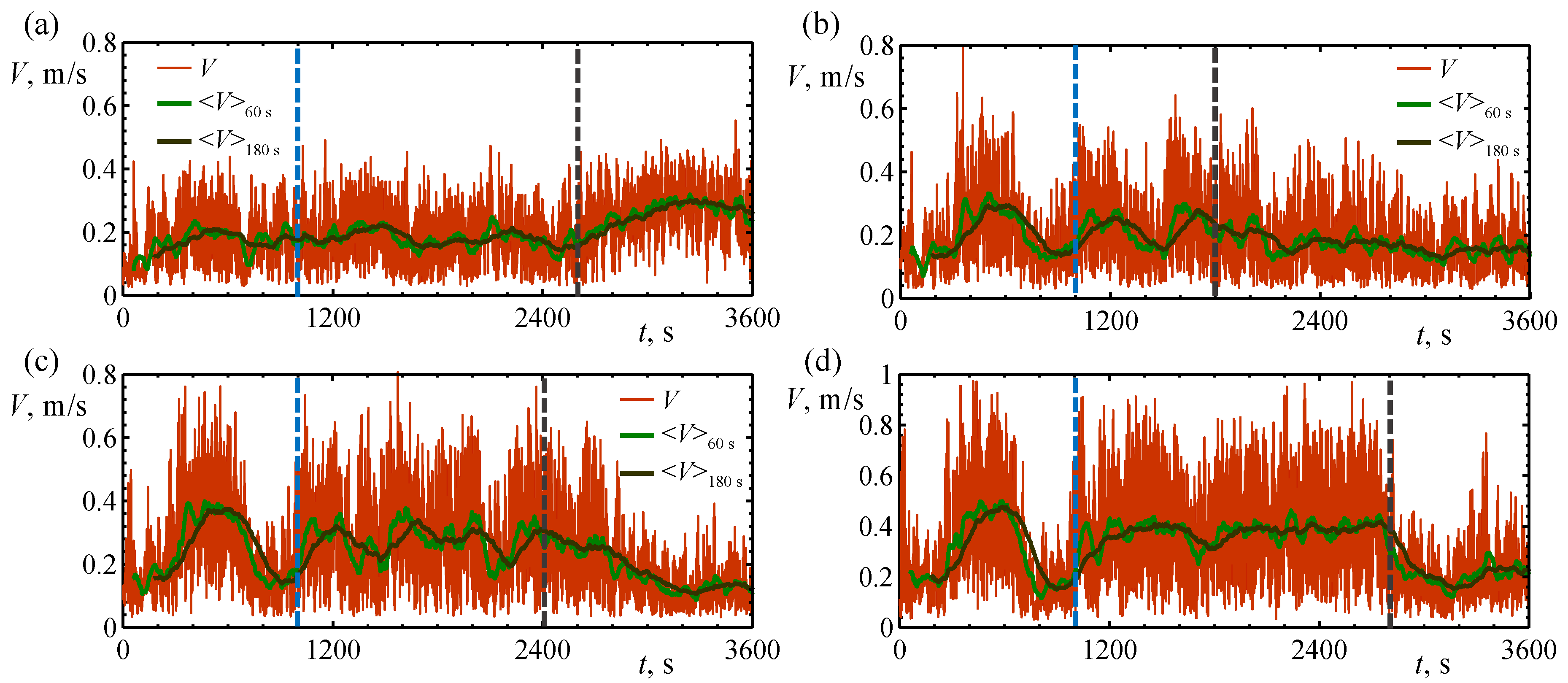
3.2. Airflow in the Room

The velocity characteristics in the occupied zone were measured during a one-hour period. However, not the whole sample could be used for analysis, as the case was non-isothermal during the whole period of measurements. Fan coils operated in a cooling mode to reduce the initial temperature and to keep the room air temperature at an approximately constant moderate level. Figure 3 presents the air temperature time variation at the four inspected points. The temperature records at all heights can be divided into 2 phases: the transient period and the quasi-steady-state period. The transient phase takes about 1000 s; the air temperature at the inspected locations drops from 32.44 ± 0.1 °C to 25.16 ± 0.2 °C. During the quasi-steady-state period the air temperature at point z = 0.1 m varies in the interval [24.7, 26.5] °C; at z = 0.6 m the interval is [24.6, 26.4] °C; at z = 1.1 m it is [24.3, 26.2] °C, and at z = 1.7 m it is [23.9, 25.9] °C. Therefore, the assessment of Tu and DR at the inspected locations was done for the temperature quasi-steady-state phase only, i.e., for the period starting from the instant of 1020 s (marked with the blue dashed line in Figure 3).

The time variation of air velocity at the inspected locations during the whole period of observation is presented in Figure 4. Besides the instantaneous velocity data (red curves), Figure 4 presents the evolution of the time-averaged air velocity with the averaging period of 1 min, <V>_{60 s} (green curves), and the averaging period of 3 min, <V>_{180 s} (black curves). The blue dashed vertical line marks the start of the temperature quasi steady-state phase of the records.

The temperature quasi-steady-state period could be divided into two sub-periods according to two different phases of the velocity behavior. At z = 1.7 m the mean air velocity (180 s long interval) has a plateau of about 0.4 m/s in the time interval [1200, 2700] s. Starting from t = 2700 s (the dark grey dashed vertical line in Figure 4d) it decreases down to 0.2 m/s during a short period of about 5 min. Relatively low velocities are detected at this point until the end of the sample. Simultaneously, an increase in the velocity is detected at z = 0.1 m (Figure 4a). At this point the mean air velocity varies around 0.18 m/s during the time interval [1200, 2580] s, and at the instant t = 2580 s a gradual increment of up to 0.3 m/s is visible. Contrary to that, at z = 0.6 m (Figure 4b) the plateau is relatively short, and a gradual decrease of the mean air velocity starts at the moment t = 1680 s, while at z = 1.1 m the plateau is longer again, and velocity reduction starts at t = 2400 s. The general conclusion from the measurement results is that in addition to the high-frequency turbulence, low frequency pulsations of the velocity field in the room exist, with a period of ten to twenty minutes or even more.

4. URANS Data on Airflow

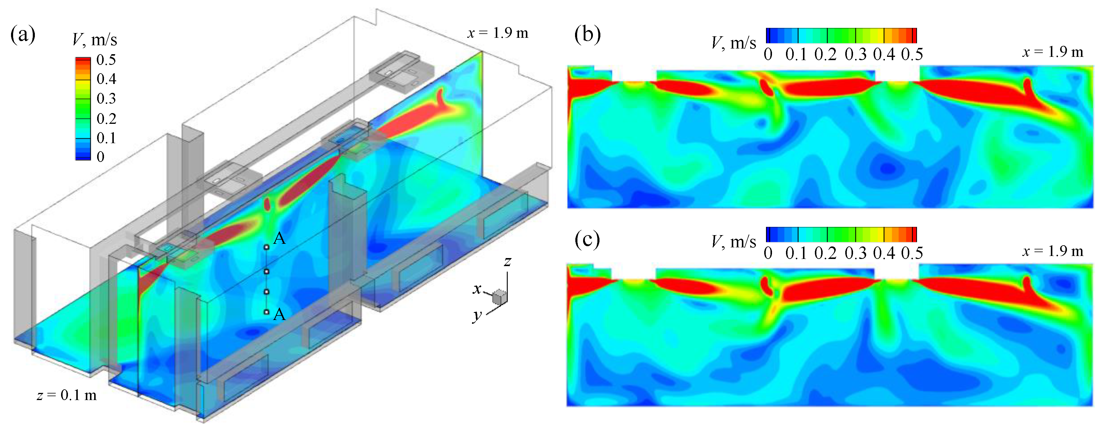
4.1. Global Unsteady Airflow Pattern

The results from the numerical simulation of the turbulent airflow in the room are shown in Figure 5. Figure 5a also illustrates the vertical line A-A placed at x = 1.9 m, y = 7.4 m; four circles mark the measurement point positions. For the flow angle θ = 25° (case #2, Table 1), the plots illustrate instantaneous velocity magnitude fields at two successive instants. Sixteen jets, supplying air to the room, form the complicated three-dimensional flow pattern. For the case with the relatively small value of θ, illustrated in Figure 5, the jets are attached to the ceiling and their positions do not change much from one time instant (Figure 5b) to another (Figure 5c). However, at a distance from fan coil supply openings, strong jet interaction is visible. The process is substantially unsteady, with visible changes in the flow field.

The vertical section, chosen for post-processing, crosses fan coil #2 (the right part of the plot) and fan coil #4 (the left part of the plot), and demonstrates the flow structure only partially. Even at this particular plot, the interaction between two and even three jets is visible. Another source of unsteadiness is the jet impingement to the sidewalls. Detailed analysis of the airflow pattern evolution through velocity field animation at various sections allows concluding that all jets undergo quasi-periodic low-frequency oscillations. Strong three-dimensional unsteadiness is also detected in the low-velocity occupied zone. Note that the used URANS approach resolves only very large eddies evolution, and all other scales (pulsations at higher frequencies) are modelled.

For the flow angle θ = 45° (case #3, Table 1) the unsteadiness is even more pronounced as the jets are detached from the ceiling and spread freely.

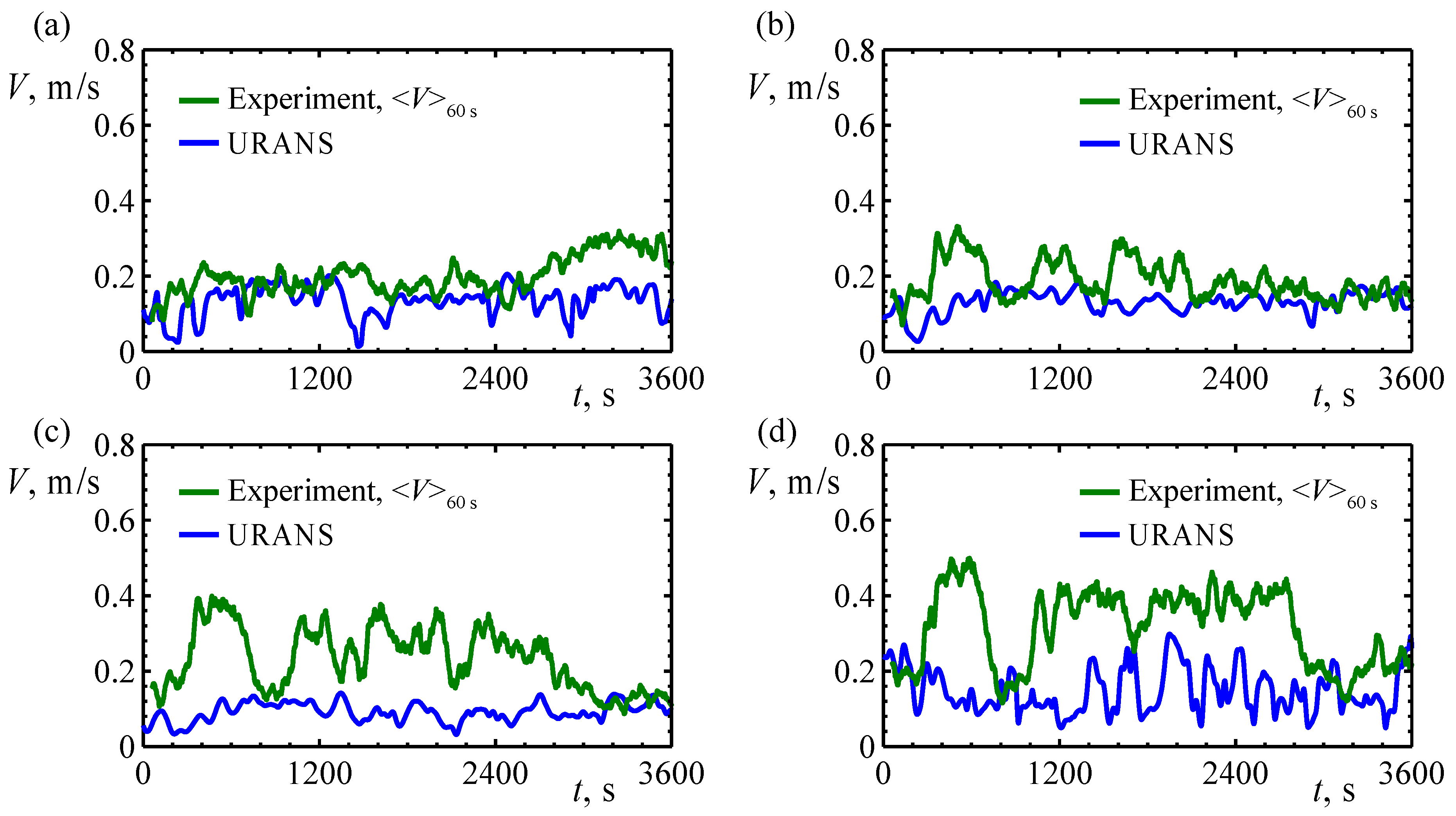
4.2. Comparison of CFD and Experimental Data

The CFD velocity magnitude data were collected at the four points for which the experimental data are available. For both the cases, the samples of 7500 s correspond to the self-oscillations with the invariant mean value, i.e., the statistically developed regime.

Figure 6 compares the evolution of computed and measured velocity magnitude for case #2, θ = 25°. The entire measured sample of one hour is given in the plot; the computed sample is presented partially. As the URANS technique resolves only low-frequency pulsations, the time-averaged measured velocity data with the averaging period of 1 min, <V>_{60 s}, are used for comparison. This type of measurement data processing filters the high frequencies that are useless for the URANS data validation. The low-frequency pulsations kept in the experimental data after processing are reproduced qualitatively in the URANS computations, though there is some quantitative difference. Thus, at the highest point, at z = 1.7 m (Figure 6d) the period of the oscillations is approximately 300 s in the numerical solution and approximately 200 s in the experimental data. The large amplitude of the measured pulsations at this point is attributed to the non-isothermal effects; if the temperature quasi-steady-state period in the time interval [1200, 2700] is considered, the measured amplitude is lower than the computed one. The amplitude of the pulsations obtained in CFD simulation is also higher than the measured amplitude at the lowest point, at z = 0.1 m (Figure 6a); the satisfactory agreement between the computed and measured frequencies is demonstrated. On the contrary, at the remaining two points higher amplitude of pulsations is obtained in the measurements. The main conclusion is that both the experimental and computational data confirm the low-frequency pulsations in the occupied zone that is very important for the thermal comfort evaluation.

The computed and measured mean velocity data are compared in Figure 7. The computed data, extracted from the time-averaged computational solution, are presented as solid lines covering the whole room height (both the jet zone and the occupied zone). The symbols illustrate all the experimental data available for the occupied zone.

The comparison performed for the two cases demonstrates perfect agreement between the measured and computed mean velocity data at the three lower points, z ≤ 1.1 m. The non-isothermal effects influence the values of <V>_{3600 s}, resulting in some increase in the values as compared with <V>_{360 s} (Figure 7a). The largest difference between the measured and computed data is seen at the highest point, z = 1.7 m. This difference could occur due to the point being not far from the jet, especially for case #3 (Figure 7b), and the non-isothermal effects could be more pronounced there.

5. Draught Rate Evaluation Discussion

According to [25], DR values could be calculated if the mean velocity magnitude, <V>, turbulent intensity, Tu, and ambient temperature, T_a, are known:

DR = (34 − T_a) (<V> − 0.05)^0.62 (0.37<V>Tu + 3.14).

(1)

In the present study, three data sets for DR evaluation are available. The first data set is from the RANS solution: the steady-state mean velocity components and Tu coupled with the temperature field. The second data set is from the URANS solution: instantaneous 3D velocity and turbulence kinetic energy fields ready for statistical analysis; URANS study is an isothermal case, and to apply Equation (1) an appropriate constant T_a value should be set. The third data set comprises results obtained with local thermo anemometer measurements: the measured values of <V>, Tu, and T_a at four points in the occupied zone.

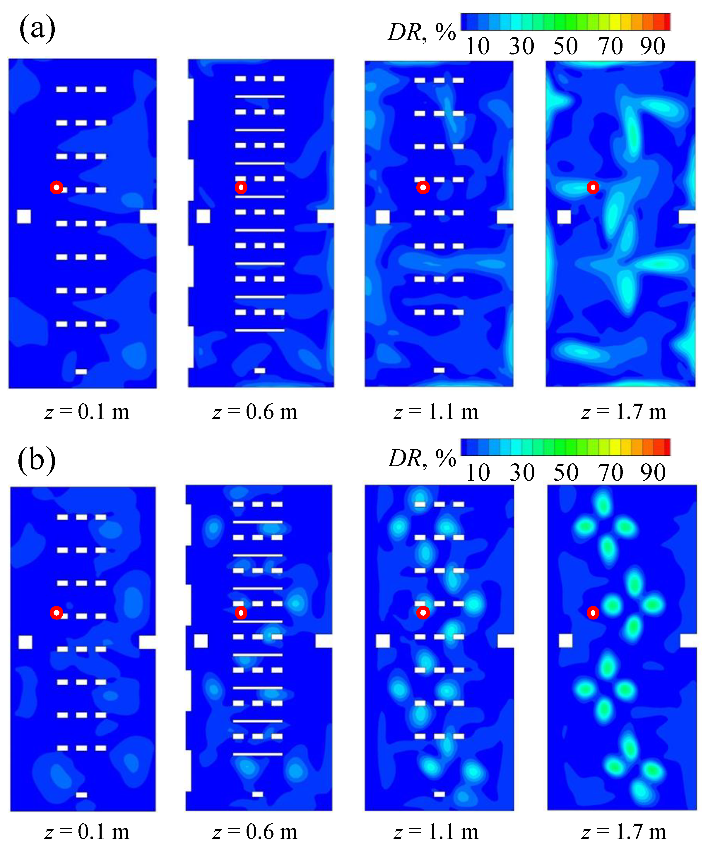
5.1. RANS-Based Draught Rate (DR) Evaluation

The calculation of DR based on the results of RANS CFD simulations is a straightforward procedure since all needed quantities (velocity, turbulence intensity, and air temperature) are provided by the solution. Steady-state distributions of DR are given in Figure 8 at the horizontal planes z = 0.1 m, z = 0.6 m, z = 1.1 m, and z = 1.7 m for two cases with θ = 25° (Figure 8a) and θ = 45° (Figure 8b).

According to the plots, the RANS-obtained DR values correspond, in general, to a small percentage of people, dissatisfied due to draught. However, the room classification differs from one level to another, and there is strong spatial non-uniformity in the distributions due to localization of the steady-state jets. At θ = 25° when the jets are attached to the ceiling (Figure 8a) at z = 0.1 m and z = 0.6 m DR ≤ 10% is detected almost everywhere (EN 16798-1:2019 category I). At z = 1.1 m there are at least two localized zones with 10% ≤ DR ≤ 20% (EN 16798-1:2019 category II). At z = 1.7 m there are several zones where 20% ≤ DR ≤ 30% (EN 16798-1:2019 category III). At θ = 45° with the detached jets (Figure 8b) the DR values are locally higher: at z = 0.1 m and z = 0.6 m DR ≤ 10% is again visible almost everywhere (EN 16798-1:2019 [28] category I), but there are several spots where 10% ≤ DR ≤ 15%. There are 16 high-DR spots at z = 1.1 m that correspond to the jet penetration locations, where 25% ≤ DR ≤ 30% there. These spots are more pronounced at z = 1.7 m, with 30% ≤ DR ≤ 35% inside the jets.

The conclusion from the engineering RANS data analysis is that the ventilation scheme used is designed well and provide satisfying DR values. However, the RANS computations provide information on mean components of velocity that define the mean velocity magnitude, or simply “velocity”. To evaluate the thermal comfort indices (and DR in particular), the time-averaged velocity magnitude, <V>, called the mean “speed” distributions, must be used [42]. It is known that in case of large velocity fluctuations that is detected for the test classroom, both in the experiments and in the unsteady computations, the “speed” values could be much higher than the “velocity” values [40].

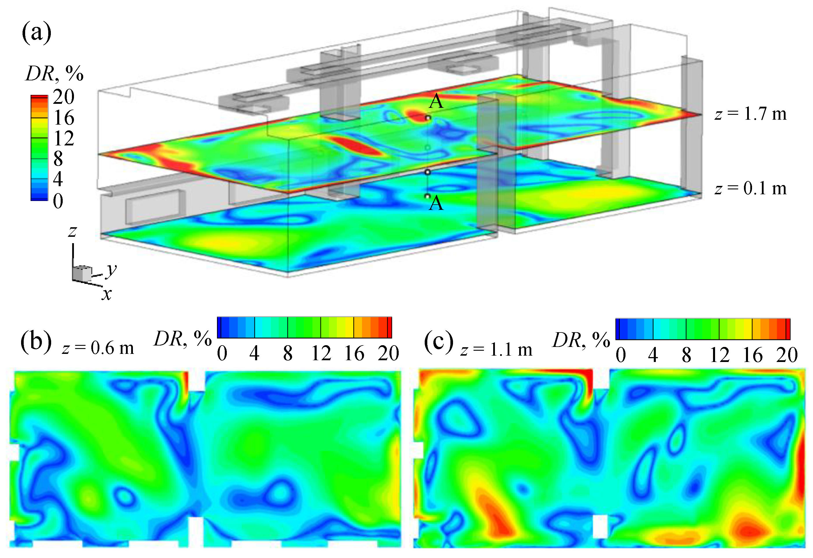
5.2. URANS-Based DR Evaluation

URANS simulations are the first step on the way of the velocity fluctuations accounting. After time-averaging, URANS data provide the 3D fields of mean velocity magnitude, <V>, and turbulent kinetic energy, k. Tu could be computed from k using the following relation: Tu = (2<k>/3)^0.5/<V>. Equation (1) could be applied to the isothermal URANS data after some temperature level is set. The DR distributions computed with the indoor air temperature taken as 27 °C are presented in Figure 9. The DR fields are plotted at the same horizontal cross-sections: z = 0.1 m, z = 0.6 m, z = 1.1 m, and z = 1.7 m. The integral DR value area-averaged over four z-planes under consideration is about 10%, but thermal comfort evaluation based on the averaged DR value is incomplete. First, it does not take into account the DR stratification visible in the occupied zone. Second, it does not take into account strong DR non-uniformity at each section, both spatial and temporal. The latter was not considered in the RANS simulation, but in the URANS fields, per the unsteady behavior of velocity distribution, discussed in Section 4.1, the DR fields are substantially unsteady.

Due to pronounced unsteady effects, the instantaneous distributions given in Figure 9 differ from the RANS-obtained fields presented in Figure 8a. In general, the URANS solution reports stronger draft discomfort than the RANS data. Thus, the spots with local values of DR exceeding 20% at two z-coordinate levels: z = 1.1 m and z = 1.7 m, change their locations from one instant to another, and the resulting high-DR zones cover a larger area as compared with the RANS data (category III in EN 16798-1:2019 [28]). The DR values exceed 10% at z = 0.1 m and z = 0.6 m (category II in EN 16798-1:2019 [28] instead of category I, resulted from the RANS data).

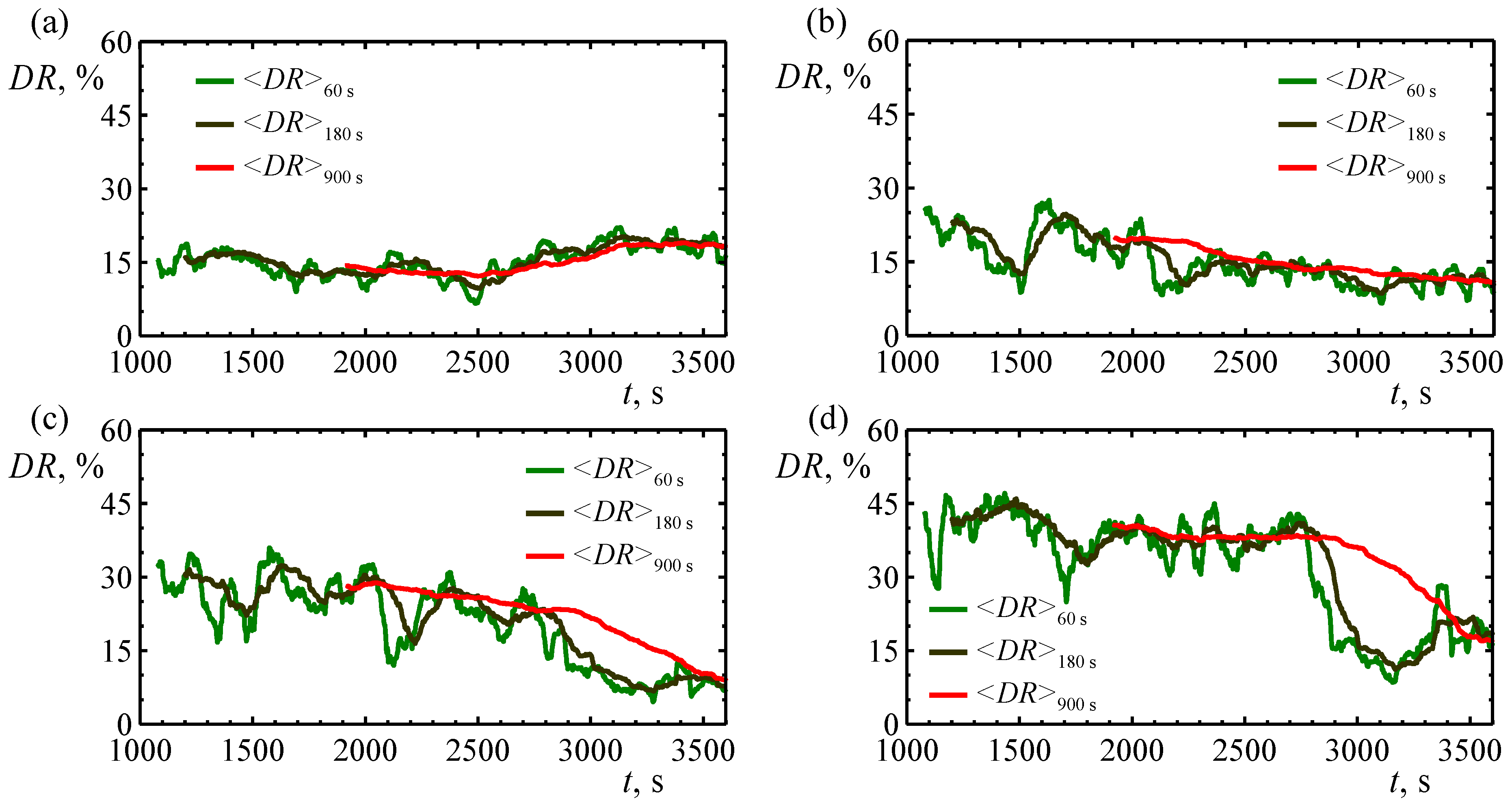
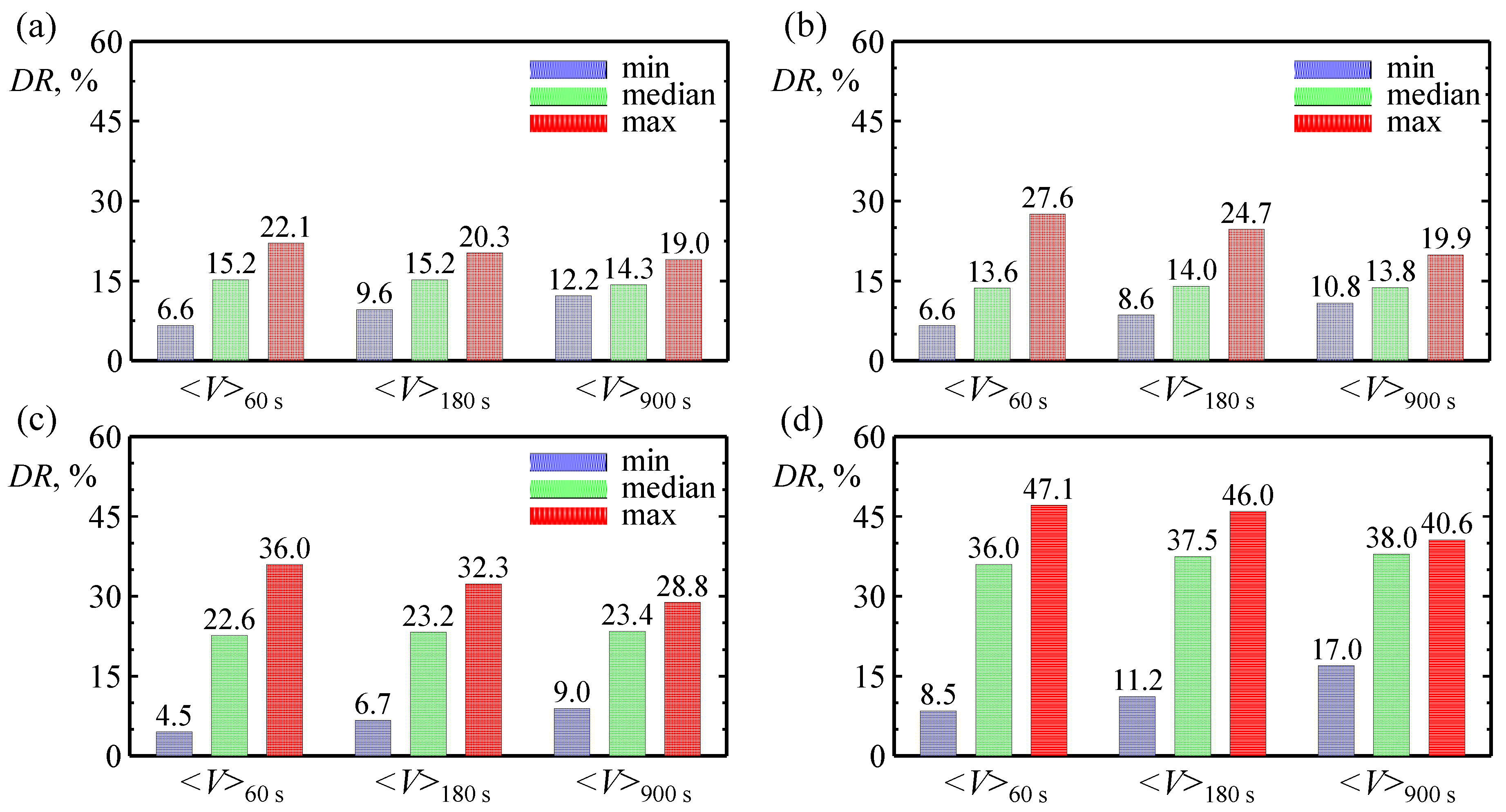
5.3. DR Evaluation Based on the Measurement Data

The measured DR time evolution curves plotted in Figure 10 represent data at four measurement points, processed with three different averaging procedures. The DR values are calculated using three moving intervals: the period of one minute, <DR>_{60 s}; the period of three minutes, <DR>_{180 s}, that corresponds to the practical procedure for evaluation of DR in ventilated spaces presented in [36]; and the period of fifteen minutes, <DR>_{900 s}, which is in coherence with the experimental protocol, reported in [25]. The data processing started at the instant of t = 1020 s (the blue dashed lines in Figure 4) that corresponds to the beginning of the temperature quasi-steady-state phase. At all z levels considered, the time-averaged DR varies in time. The DR evolution reproduces to some extent the unsteady velocity behavior, presented previously in Figure 4 and Figure 6: characteristic periods of 200–300 s are registered for the two quantities. It is evident that the DR assessment depends much on the averaging period. Remarkably that for the longest averaging period of 900 s, the time-averaged DR values also change in time significantly, see the red curve, especially at z = 0.6 m (Figure 10b) and z = 1.7 m (Figure 10d).

In addition to the time evolution curves, Figure 11 presents the integral range of the DR time variation: for three intervals of averaging (60 s, 180 s, 900 s) the minimum, maximum, and median values over the thermal quasi-steady-state period are given. With the increase in the averaging interval, the range of DR variation becomes narrower. The minimum value grows up, the maximum value decreases, while the mean and the median values remain almost the same for the whole temperature quasi-steady-state period. At each level, the difference between the maximum DR and minimum DR is the lowest for the 900 s long interval; this difference varies from one point to another: at z = 1.7 m this difference is 23.6%, at z = 1.1 m it is 9.1%, at z = 0.6 m it is 19.8%, and at z = 0.1 m it is 6.8%. For the three intervals of assessment, the maximum difference between the DR median values is observed at z = 1.7 m, where the median value of <DR>_{60 s} is 2.0% lower than that of <DR>_{900 s}.

The conclusion is that it is necessary to pay much attention to the measurement period for a reliable DR estimation. If the median values from a set of numerous measurements are used, the DR assessment interval for the room under consideration could be 180 s long since median values for <DR>_{180 s} and <DR>_{900 s} are practically equal. However, for the practical categorization of the room, it is insufficient, as a single measurement of 180 s long could be performed during a high-DR or low-DR period and the input used for categorization would be far from the median. The recommendation for the averaging period choice is that the range of variation of DR, i.e., the difference between the maximum and the minimum <DR> values, for the sufficient averaging period, must be lower than 10% of the median value. Note that among the four points under consideration, at two points this condition is not fulfilled even for the longest period of 900 s (see Figure 11c,d).

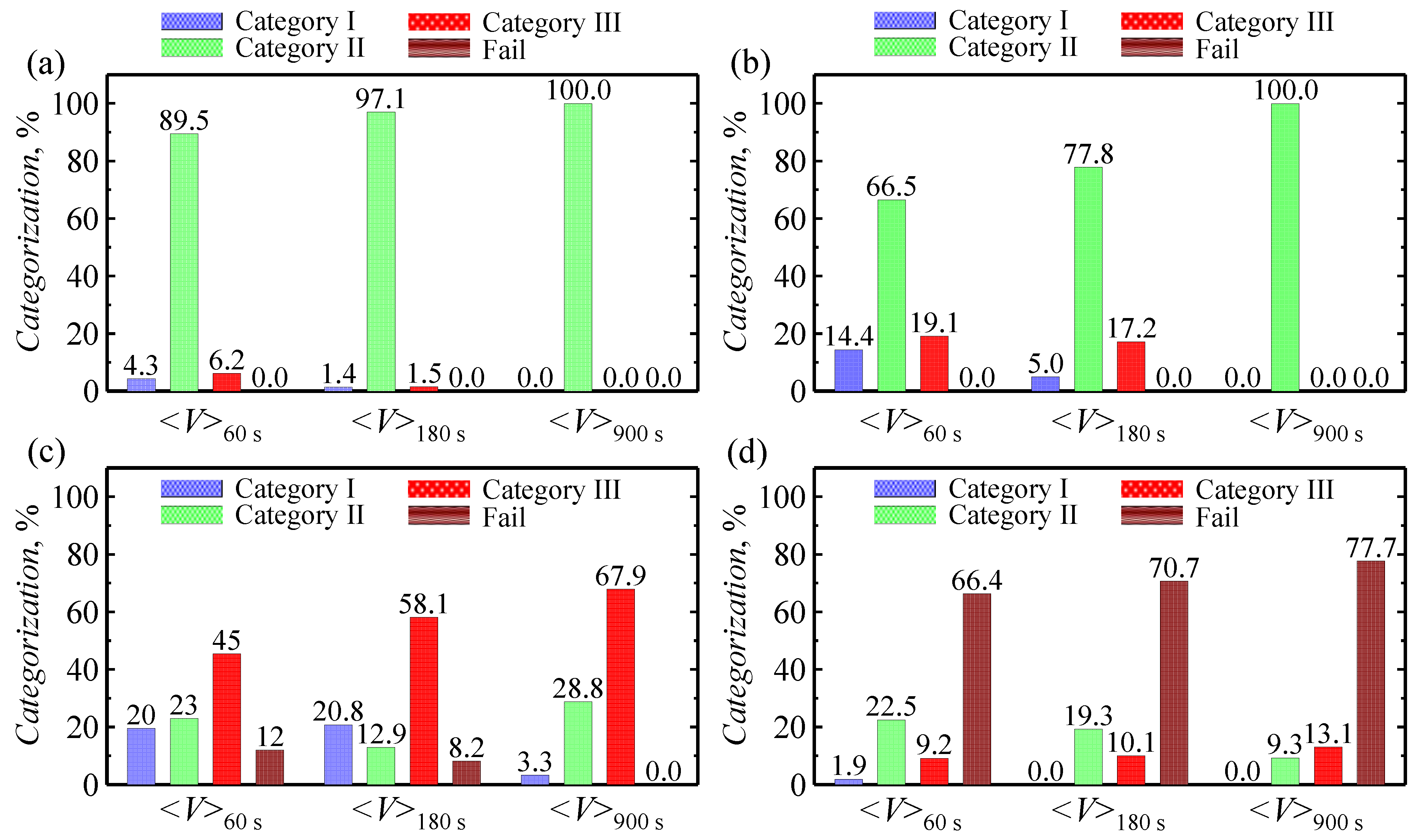
5.4. Categorization of the Classroom Environment Based on Measured DR

Information for the categorization for DR at the monitored locations is presented in Figure 12. At the monitored location, based, for example, on the measured data at z = 1.1 m, the probability to categorize the thermal environment with respect to DR, using a 60 s long interval for assessment, is as follows: 19.6% as Category I, 23.0% as Category II, and 45.4% as Category III. A probability of 12.0% exists that the categorization evaluated at this point does not meet the requirements of the standard (categorization is attributed to be “Fail”). If 900 s long intervals are used for measurements at the same point, there is no probability of the DR categorization to be assessed as “Fail”. This example shows both the importance of the long-term measurements for assessment of the thermal environment with respect to DR and the way of how to cope with the draught complaints.

6. Conclusions

The paper presents the results of a combined numerical and experimental study of room air movement in a test university classroom with a controlled indoor environment. Both the 3D field results computed with the unsteady RANS technique and the real-scale long-term point velocity data measured with the thermo anemometer report about strong unsteadiness of the airflow. Low-frequency high-amplitude velocity fluctuations emerging due to airflow instability lead to strong time variation of the draught rate that corresponds to possible uncertainty in the percentage of dissatisfied persons due to unwanted local cooling/heating related to draught.

For large indoor spaces with numerous interacting air supply jets, it is recommended to assess DR based on time records of both air velocity and air temperature not shorter than half an hour. The categorization procedure must be done for a sufficiently long interval. The recommendation/guidance of such kind must be given in the standards since not all people dealing with categorization and assessment of the indoor thermal environment are professionals in the field of fluid mechanics. However, as it is not possible to specify a universal length of the time interval for the DR assessment procedure in case of a low-frequency unsteadiness occurs, a preliminary study of the DR sensitivity to the averaging period should be done during a categorization procedure.

In case of categorization of the thermal environment, the time-point measurements or steady-state RANS computations would lead to wrong conclusions as well as they cannot be used for identification of the reasons for complaints due to draught discomfort, if strong unsteadiness of the airflow is expected. In general, the presented analyses demonstrated the importance of the combination of the unsteady computer simulations and long-term measurements for the correct assessment of both DR and thermal comfort, as well as for the proper categorization of the indoor thermal environment.

The general recommendation is to perform measurements and simulations under design conditions, with respect to both occupancy and mode of operation. If geometry details and occupants are modelled in an engineering study, the grid has to be coarse to reduce the computational cost. Even in this case, the CFD problem formulation must be unsteady, and the turbulence model and the quality of the mesh must be sufficient to reproduce the main low-frequency pulsations. A study of the DR variation effects in case of an indoor space is filled with the furniture and occupants is planned as future work.

To summarize, the DR assessment must be done for a sufficiently long interval allowing identification of the velocity field variations and the DR variation in the interval for assessment should be as small as possible. However, even if these conditions are fulfilled, the indoor space categorization could be uncertain, e.g., the indoor space could be related to different categories for successive relatively long periods of time. It is necessary to investigate what happens with the occupant’s complaints if categorization in an indoor space varies in time. Thus, additional research is needed on how people perceive the thermal environment under the low-frequency unsteadiness. Analysis of the possible complaints about the thermal environment that cannot be discovered by local short-time measurements is also a field for future work.

References

1. Sakellaris, I.; Saraga, D.; Mandin, C.; de Kluizenaar, Y.; Fossati, S.; Spinazzè, A.; Cattaneo, A.; Szigeti, T.; Mihucz, V.; de Oliveira Fernandes, E.; et al. Personal Control of the Indoor Environment in Offices: Relations with Building Characteristics, Influence on Occupant Perception and Reported Symptoms Related to the Building—The Officair Project. Appl. Sci. 2019, 9, 3227. [Google Scholar] [CrossRef] [Green Version]
2. Branco, P.T.B.S.; Alvim-Ferraz, M.C.M.; Martins, F.G.; Sousa, S.I.V. Quantifying indoor air quality determinants in urban and rural nursery and primary schools. Environ. Res. 2019, 176, 108534. [Google Scholar] [CrossRef] [PubMed]
3. Chen, Y.; Chen, B. The Combined Effect of Indoor Air Quality and Socioeconomic Factors on Health in Northeast China. Appl. Sci. 2019, 10, 2827. [Google Scholar] [CrossRef] [Green Version]
4. Olesen, B.; Bluyssen, P.; Roulet, C.A. Ventilation and Indoor Environmental Quality; Taylor & Francis: Abingdon, UK, 2007; pp. 62–105. [Google Scholar]
5. van Dijken, F.; van Bronswijk, J.E.M.H.; Sundell, J. Indoor environment in Dutch primary schools and health of the pupils. Build. Res. Inform. 2006, 34, 437–446. [Google Scholar] [CrossRef]
6. Holcomb, L.C.; Pedelty, J.F. Comparison of employee upper respiratory absenteeism costs with costs associated with improved ventilation. ASHRAE Trans. 1994, 100, 914–921. [Google Scholar]
7. Schreuder, E.; van Heel, L.; Goedhart, R.; Dusseldorp, E.; Schraagen, J.M.; Burdorf, A. Effects of newly designed hospital buildings on staff perceptions: A pre-post study to validate design decisions. HERD Health Environ. Res. Des. J. 2015, 8, 77–97. [Google Scholar] [CrossRef]
8. Bode, F.I.; Croitoru, C.V.; Dogeanu, A.M.; Nastase, I. Thermal comfort and IEQ assessment of an under-floor air distribution system. In Proceedings of the BS2013 Conference, Chambéry, France, 26–28 August 2013; pp. 2334–23399. [Google Scholar]
9. Dhalluin, A.; Limam, K. Comparison of natural and hybrid ventilation strategies used in classrooms in terms of indoor environmental quality, comfort and energy savings. Indoor Built Environ. 2014, 23, 527–542. [Google Scholar] [CrossRef]
10. Rohdin, P.; Molin, A.; Moshfegh, B. Experiences from nine passive houses in Sweden–Indoor thermal environment and energy use. Build. Environ. 2014, 71, 176–185. [Google Scholar] [CrossRef] [Green Version]
11. ISO 7730. Ergonomics of the Thermal Environment. Analytical Determination and Interpretation of Thermal Comfort Using Calculation of the PMV and PPD Indices and Local Thermal Comfort Criteria; International Organization for Standardization: Geneva, Switzerland, 2005. [Google Scholar]
12. Gendelis, S.; Jakovičs, A.; Ratnieks, J. Thermal comfort condition assessment in test buildings with different heating/cooling systems and wall envelopes. Energy Procedia 2017, 132, 153–158. [Google Scholar] [CrossRef]
13. Simone, A.; Della Crociata, S.; Martellotta, F. The influence of clothing distribution and local discomfort on the assessment of global thermal comfort. Build. Environ. 2013, 59, 644–653. [Google Scholar] [CrossRef]
14. Mumovic, D.; Palmer, J.; Davies, M.; Orme, M.; Ridley, I.; Oreszczyn, T.; Judd, C.; Critchlow, R.; Medina, H.A.; Pilmoor, G.; et al. Winter indoor air quality, thermal comfort and acoustic performance of newly built secondary schools in England. Build. Environ. 2009, 44, 1466–1477. [Google Scholar] [CrossRef]
15. Kiil, M.; Mikola, A.; Thalfeldt, M.; Kurnitski, J. Thermal comfort and draught assessment in a modern open office building in Tallinn. In E3S Web of Conferences; EDP Sciences: Les Ulis, France, 2019; Volume 111. [Google Scholar]
16. Kiil, M.; Simson, R.; Thalfeldt, M.; Kurnitski, J. A comparative study on cooling period thermal comfort assessment in modern open office landscape in Estonia. Atmosphere 2020, 11, 127. [Google Scholar] [CrossRef] [Green Version]
17. Koper, P.; Lipska, B.; Michnol, W. Assessment of thermal comfort in an indoor swimming pool making use of the numerical prediction CFD. Archit. Civ. Eng. Environ. 2010, 3, 95–104. [Google Scholar]
18. Deng, X.; Tan, Z. Numerical analysis of local thermal comfort in a plan office under natural ventilation. Indoor Built Environ. 2019, 1420326X19866497. [Google Scholar] [CrossRef]
19. Fanger, P.O.; Christensen, N.K. Perception of draught in ventilated spaces. Ergonomics 1986, 29, 215–235. [Google Scholar] [CrossRef]
20. Griefahn, B.; Künemund, C.; Gehring, U. The impact of draught related to air velocity, air temperature and workload. Appl. Ergon. 2001, 32, 407–417. [Google Scholar] [CrossRef]
21. Hens, H.S. Thermal comfort in office buildings: Two case studies commented. Build. Environ. 2009, 44, 1399–1408. [Google Scholar] [CrossRef]
22. Olesen, B.; D’Ambrosio-Alfano, F.R.; Parsons, K.C.; Palella, B.I. The history of international standardization for the ergonomics of the thermal environment. In Proceedings of the 9th International Windsor Conference, Cumberland Lodge, Windsor, UK, 7–10 April 2016; pp. 7–10. [Google Scholar]
23. Lampret, Ž.; Krese, G.; Butala, V.; Prek, M. Impact of airflow temperature fluctuations on the perception of draught. Energy Build. 2018, 179, 112–120. [Google Scholar] [CrossRef]
24. Abid, H.; Baklouti, I.; Driss, Z.; Bessrour, J. Experimental and numerical investigation of the Reynolds number effect on indoor airflow characteristics. Adv. Build. Energy Res. 2019, 1–26. [Google Scholar] [CrossRef]
25. Fanger, P.O.; Melikov, A.K.; Hanzawa, H.; Ring, J. Air turbulence and sensation of draught. Energy Build. 1988, 12, 21–39. [Google Scholar] [CrossRef]
26. Pinto, D.; Rocha, A.; Simões, M.L.; Almeida, R.M.; Barreira, E.; Pereira, P.F.; Ramos, N.M.; Martins, J.P. An innovative approach to evaluate local thermal discomfort due to draught in semi-outdoor spaces. Energy Build. 2019, 203, 109416. [Google Scholar] [CrossRef]
27. American Society of Heating; Refrigerating and Air-Conditioning Engineers. Thermal Environmental Conditions for Human Occupancy: ANSI/ASHRAE Standard 55-2017; ASHRAE: Peachtree Corners, GA, USA, 2017. [Google Scholar]
28. EU Standard 16798-1. Energy Performance of Buildings—Ventilation for Buildings—Part 1; International Organization for Standardization: Geneva, Switzerland, 2019. [Google Scholar]
29. Zhai, Z.J.; Zhang, Z.; Zhang, W.; Chen, Q.Y. Evaluation of various turbulence models in predicting airflow and turbulence in enclosed environments by CFD: Part 1—Summary of prevalent turbulence models. HVAC R Res. 2007, 13, 853–870. [Google Scholar] [CrossRef]
30. Thool, S.B.; Sinha, S.L. Simulation of room airflow using CFD and validation with experimental results. Int. J. Eng. Sci. Technol. 2014, 6, 192. [Google Scholar]
31. Risberg, D.; Vesterlund, M.; Westerlund, L.; Dahl, J. CFD simulation and evaluation of different heating systems installed in low energy building located in sub-arctic climate. Build. Environ. 2015, 89, 160–169. [Google Scholar] [CrossRef]
32. Hirsch, C.; Tartinville, B. Reynolds-Averaged Navier-Stokes modelling for industrial applications and some challenging issues. Int. J. Comput. Fluid Dyn. 2009, 23, 295–303. [Google Scholar] [CrossRef]
33. Koskela, H.; Heikkinen, J. Calculation of thermal comfort from CFD-simulation results. In Proceedings of the International Conference on Indoor Air Quality and Climate, Monterey, CA, USA, 30 June–5 July 2002; Volume 3, pp. 712–717. [Google Scholar]
34. Li, Y.; Nielsen, P.V. CFD and ventilation research. Indoor Air 2011, 21, 442–453. [Google Scholar] [CrossRef]
35. Ivanov, N.G.; Zasimova, M.A. Mean air velocity correction for thermal comfort calculation: Assessment of velocity-to-speed conversion procedures using Large Eddy Simulation data. J. Phys. Conf. Ser. 2018, 1135, 012106. [Google Scholar] [CrossRef]
36. Markov, D. Practical evaluation of the thermal comfort parameters. In Proceedings of the First Annual International Course: Ventilation and Indoor climate, Pamporovo, Bulgaria, 21–25 October 2002. [Google Scholar]
37. Ivanov, N.; Zasimova, M.; Smirnov, E.; Abramov, A.; Markov, D.; Stankov, P. Unsteady RANS Simulation of Air Distribution in a Ventilated Classroom with Numerous Jets. E3S Web Conf. 2019, 111, 02010. [Google Scholar] [CrossRef] [Green Version]
38. ISO 7726. Ergonomics of the Thermal Environment—Instruments for Measuring Physical Quantities; International Organization for Standardization: Geneva, Switzerland, 1998. [Google Scholar]
39. Kosutova, K.; Van Hoof, T.; Vanderwel, C.; Bloocken, B.; Hensen, J. Cross-ventilation in a generic isolated building equipped with louvers: Wind-tunnel experiments and CFD simulations. Build. Environ. 2019, 154, 263–280. [Google Scholar] [CrossRef]
40. Ivanov, N.G.; Zasimova, M.A.; Smirnov, E.M.; Markov, D. Evaluation of mean velocity and mean speed for test ventilated room from RANS and LES CFD modeling. E3S Web Conf. 2019, 85, 02004. [Google Scholar] [CrossRef]
41. Mijorski, S.G.; Markov, D.G.; Pichurov, G.T.; Stankov, P.; Ivanov, N.G.; Simova, I.S. CFD based design of a ventilated space. In IOP Conference Series: Materials Science and Engineering; IOP Publishing: Bristol, UK, 2019; Volume 618, p. 012049. [Google Scholar]
42. Koskela, H.; Heikkinen, J.; Niemela, R.; Hautalampi, T. Turbulence correction for thermal comfort calculation. Build. Environ. 2001, 36, 247–255. [Google Scholar] [CrossRef]
Figure 1. (a) Geometry model for Unsteady RANS (URANS), (b,c) room interior photos with four fan coils numbered, (d) photo near a fan coil.
Applsci 10 05036 g001
Figure 2. Time evolution of measured velocity at four points located near four supply sections: (a) east, (b) south, (c) west, and (d) north of fan coil #4.
Applsci 10 05036 g002
Figure 3. Air temperature time variation at the inspected points.
Applsci 10 05036 g003
Figure 4. Evolution of velocity at the inspected points: (a) z = 0.1 m, (b) z = 0.6 m, (c) z = 1.1 m, (d) z = 1.7 m.
Applsci 10 05036 g004
Figure 5. Instantaneous velocity magnitude at various cross-sections in two moments of time: (a,b) t = t0 and (c) t = t0 + 5000 s (data for θ = 25°, case #2).
Applsci 10 05036 g005
Figure 6. Time evolution of velocity magnitude at four monitoring points: (a) z = 0.1 m, (b) z = 0.6 m, (c) z = 1.1 m and (d) z = 1.7 m (data for θ = 25°, experimental case #1 and computational case #2).
Applsci 10 05036 g006
Figure 7. Comparison of the computed mean velocity profile with the experimental data, (a) θ = 25°, case #2, and (b) θ = 45°, case #3.
Applsci 10 05036 g007
Figure 8. RANS-computed fields of draught rate (DR) at four cross-sections of the room for two cases: (a) θ = 25° and (b) θ = 45°; red circles indicate the A-A vertical line position.
Applsci 10 05036 g008
Figure 9. Unsteady RANS (URANS)-obtained instantaneous distributions of DR values at four cross-sections of the room (data for θ = 25°, case #2).
Applsci 10 05036 g009
Figure 10. Time evolution of DR at four monitoring points: (a) z = 0.1 m, (b) z = 0.6 m, (c) z = 1.1 m, and (d) z = 1.7 m (data for θ = 25°, case #1).
Applsci 10 05036 g010
Figure 11. Range of DR variation for three different averaging periods at four monitoring points: (a) z = 0.1 m, (b) z = 0.6 m, (c) z = 1.1 m, and (d) z = 1.7 m (data for θ = 25°, case #1).
Applsci 10 05036 g011
Figure 12. Categorization of the classroom environment, based on measured DR time variation: (a) z = 0.1 m, (b) z = 0.6 m, (c) z = 1.1 m, and (d) z = 1.7 m (data for θ = 25°, case #1).
Applsci 10 05036 g012