Techno-Economic Analysis of a Solar Thermal Plant for Large-Scale Water Pasteurization

Abstract

Water pasteurization has the potential to overcome some of the drawbacks of more conventional disinfection techniques such as chlorination, ozonation and ultraviolet radiation treatment. However, the high throughput of community water systems requires energy-intensive processes, and renewable energy sources have the potential to improve the sustainability of water pasteurization plants. In case of water pasteurization by solar thermal treatment, the continuity of operation is limited by the intermittent availability of the solar irradiance. Here we show that this problem can be addressed by a proper design of the plant layout, which includes a thermal energy storage system and an auxiliary gas boiler. Based on a target pasteurization protocol validated by experiments, a complete lumped-component model of the plant is developed and used to determine the operating parameters and size of the components for a given delivery flow rate. Finally, we report an economic analysis of the proposed plant layout, which allows its optimization for different scenarios based on two design variables, namely the solar multiple and the duration of the thermal energy storage. Based on the analyzed cases, it is found that the proposed plant layouts may yield a unit cost of water treatment ranging from ≈32 EUR-cents m⁻³ to ≈25 EUR-cents m⁻³.

1. Introduction

High quality standards for drinkable water supply are essential to health protection and personal hygiene [1]. Securing safety of drinking water is particularly critical in large-scale community distribution, to prevent outbreaks of waterborne diseases [2]. Community water systems, in general, mostly resort to groundwater sources, where the major contaminants may include: heavy metals, such as arsenic, cadmium, chromium, nickel and lead; organic compounds, such as chloroform, gasoline, pesticides and herbicides; pathogens, such as protozoa, bacteria and viruses and emerging pollutants [3,4,5]. Water treatment lines must be then properly designed to eliminate specific target contaminants, which generally require different purification techniques and protocols [6,7,8]. In this sense, microbiological inactivation—i.e., disinfection—accounts for most violations with respect to the prescribed quality standards [3].

Conventional water disinfection technologies rely on chlorination, ozonation and treatment by ultraviolet (UV) radiation [9]. Chlorination is one of the most effective techniques and, thanks to the reduced operational costs, is widely adopted. Water disinfection is obtained by the hypochlorous acid formed from chlorine when introduced in water. However, chlorination may give rise to disinfection by-products that could be harmful to the human health and environment, besides affecting the taste and smell of the treated water [10,11]. Ozonation represents a valid alternative to chlorination, thanks to its increased effectiveness against viruses and bacteria. In addition, ozone increases the dissolved oxygen, improving the water quality. However, ozone is corrosive, extremely irritating and eventually toxic, very sensitive to dosages and not cheap [12,13]. Finally, UV treatment inactivates the exposed microorganisms and viruses by damaging their DNA/RNA, which reduces their functionality and ability to reproduce. This treatment has the advantage to avoid harmful by-products; however, it requires important capital and operational costs for electricity and consumables [14,15].

An alternative method to overcome some of the drawbacks of the previous techniques relies on the use of heat for water treatment, commonly known as pasteurization. This method has been traditionally adopted for inactivation of pathogens and microorganisms in milk and food. Heating is indeed effective in eliminating pathogens; however, this effectiveness strongly depends on the treatment temperature and exposure time [16,17]. The high throughput of modern systems for community water treatment typically requires short treatment times, thus resulting in higher temperatures and thus energy-intensive processes. In this sense, renewable energy sources and waste-heat recovery have the potential to reduce the environmental footprint and allow design of sustainable water treatments, as already demonstrated in a variety of different applications [18,19,20,21,22,23].

In the case of solar thermal energy, continuous water processing is limited by the intermittent availability of the solar irradiance. This issue can be overcome using thermal energy storage [24,25,26] and ancillary power units, opportunely integrated in the plant layout. In this view, here we develop a complete lumped-component model of large-scale solar thermal water disinfection based on a pasteurization protocol validated by experiments. This model is employed to size the components of the plant and determine its operating parameters given the mass flow rate of water to be treated. We also report an economic analysis of the proposed plant layout, which allows to optimize the unit cost of water purification based on specific design variables.

The article is organized as follows. In Section 2 we first select and experimentally test the target pasteurization protocol. In Section 3 we develop the plant model and discuss its technical implementation. Section 4 is dedicated to the economic analysis of the proposed solutions for different possible scenarios. Finally, the conclusions are drawn in Section 5.

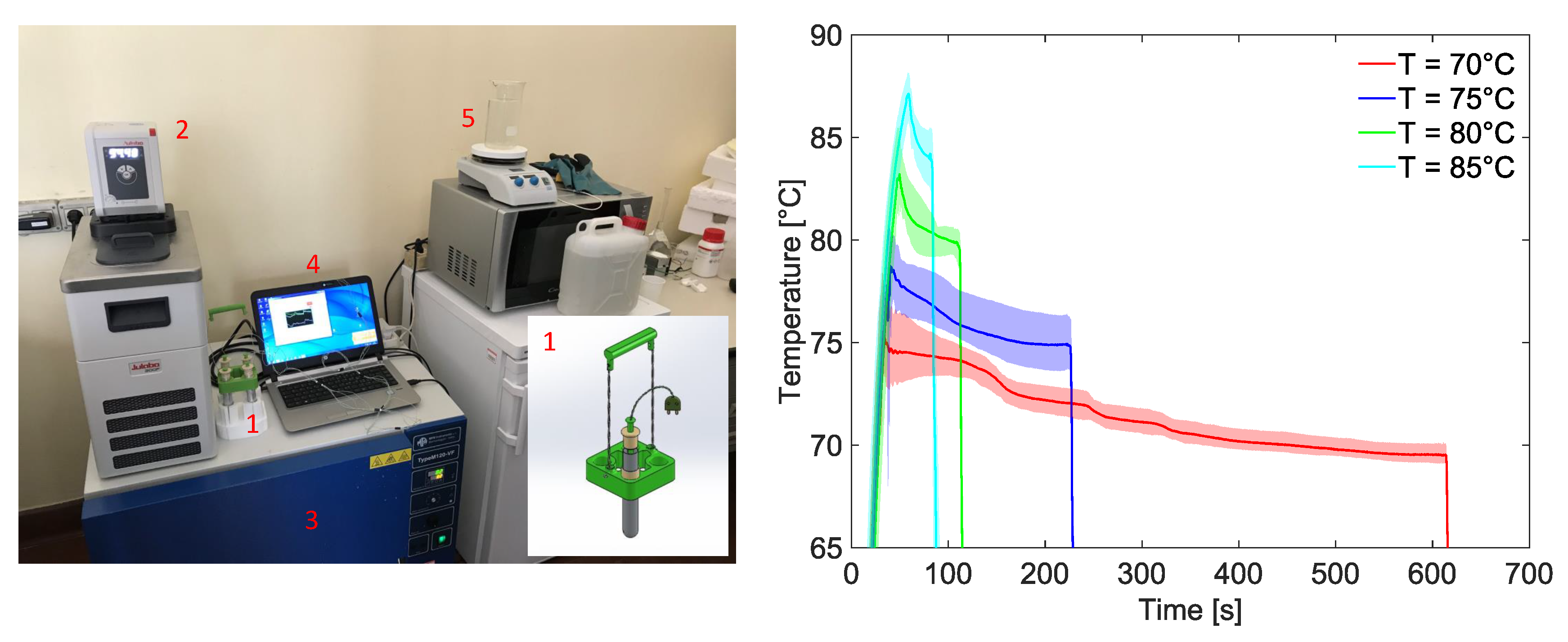
2. Experimental Pasteurization Tests

The starting point for the design and optimization of the solar thermal plant for water treatment is the identification of the target operating parameters for the pasteurization protocol. In this section, we experimentally test the effectiveness of different protocols for water pasteurization, which will be then employed to build the lumped-component model of the plant. The key parameters, that is, the treatment temperature and the residence time, are commonly chosen according to the Safety Zone in the temperature-time diagram for water pasteurization [27], which allows to easily identify the proper treatment to be adopted according to the target pathogens to inactivate. Here, we consider one point on the inactivation curve for enteric viruses (540 s at $70{}^{\circ }$C), which is the most conservative choice for short-time pasteurization processes, and other three points obtained by regression at higher temperatures (114 s at $75{}^{\circ }$C, 30 s at $80{}^{\circ }$C and 8 s at $85{}^{\circ }$C).

The set up for the experimental tests has been designed considering two main requirements: water has to be maintained at uniform temperature during the pasteurization; the heating up phase of water to the treatment temperature has to be fast, to avoid spurious effects on the observed disinfection results. The equipment for the experimental pasteurization tests is shown in Figure 1 (left). Four aluminum test tubes—positioned into a tailor-made 3D-printed bracket (1) to easily handle the water samples during the experiment (see a detail of the CAD drawing in the inset)—allow to carry out four repetitions per test. Each tube is filled with a reduced amount of sample water per test (10 mL) to reduce thermal inertia during the tests. The temperature of each sample is measured using a thermocouple (K-type, RS Pro [28]; temperature range –75 to $260{}^{\circ }$C and accuracy ±$1.5{}^{\circ }$C), which is positioned at the center of the water sample using a tailor-made 3-D printed gasket. This latter gasket has been designed to hold the tip of the thermocouple in the bulk water, thus measuring the mean temperature of the sample. All the thermocouples are connected to a laptop (4) for digital acquisition of the temperature signals (LabVIEW©, National Instruments, Austin, TX, USA). The water samples are first heated up quickly to the target treatment temperature using a (2) thermostatic water bath (CORIO CD-300F, Julabo, Seelbach, Germany), which is maintained at a controlled temperature of $95{}^{\circ }$C. The samples are then quickly moved into (3) an industrial furnace for thermostatic applications (TypeM120-VF, MPM Instruments, Bernareggio, Italy), which is maintained at the tested treatment temperature and used for the pasteurization. After the target resident time, an ice bucket is used to cool down the water samples to the environment temperature. Each test is repeated three times, in order to obtain the necessary amount of water for the microbiological analysis of the results (provided by the SMAT laboratories in Torino, Italy). All the tools in contact with the water samples (i.e., aluminum tubes, thermocouples and related brackets) are sanitized after each test, by immersing them for 120 s into a beaker filled with 700 mL of water maintained at a constant temperature of $95{}^{\circ }$C thanks to a (5) digital hot plate stirrer (AREX Digital, VELP Scientifica, Usmate Velate MB, Italy).

The temperature of the water samples during the experimental tests for the four selected pasteurization protocols are shown in Figure 1 (right). The solid lines represent the average value of the four repetitions for one protocol, while the semi-transparent band the minimum–maximum range observed. The three stages of the adopted thermal protocol can be clearly noticed from the reported temperature transients. The steep initial temperature increase corresponds to the rapid pre-heating in the thermostatic bath, followed by the pasteurization in the oven at nearly constant temperature and by the fast cooling to ambient conditions. Notice that, in the experiments, the average pasteurization temperature is kept for at least 582 s at ≈$71{}^{\circ }$C, 185 s at ≈$76{}^{\circ }$C, 60 s at ≈$81{}^{\circ }$C and 23 s at ≈$85{}^{\circ }$C, therefore achieving the target treatment time with some tolerance.

The bacterial load (in terms of total coliforms and Escherichia coli) is provided according to the Most Probable Number (MPN [29]) method using a Colilert Quanti-Tray 2000 assay (IDEXX). Starting from an initial bacterial load in the raw water samples (taken from the Po river in Torino) of 2419.6 and 143.9 MPN of total coliforms and Escherichia coli per 100 mL, respectively, the results of the microbiological analysis on the treated samples show no residual bacteria in all cases (up to the detection limit of the tests, i.e., <1 MPN/100 mL). Therefore, each pasteurization protocol confirms its effectiveness in eliminating water pathogens. In the following, we adopt the 114 s at $75{}^{\circ }$C protocol for the model design of the plant, since it represents a good compromise between the required temperature and resident time to be realized in a solar thermal plant.

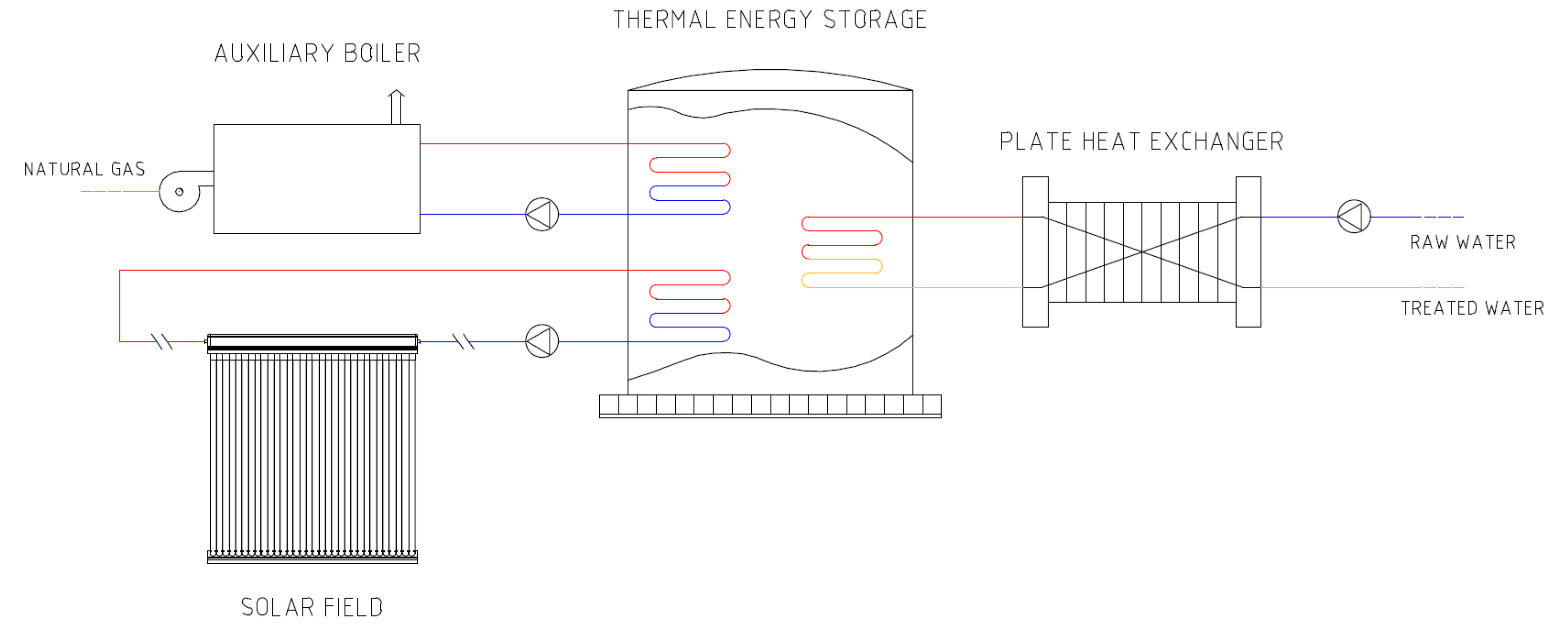
3. Plant Model Design

An overview of the plant layout for the solar thermal water treatment is shown in Figure 2. The pasteurization takes place in the coil immersed in the thermal energy storage tank, where the target treatment temperature must be maintained. The required thermal energy is provided by the solar thermal collectors together with an auxiliary boiler, which is employed as backup heat supplier to levelize the intermittent nature of solar source. To reduce the utilization of the auxiliary boiler and better exploit the intermittent solar source, the system includes a sensible heat storage [30] system that allows to maintain a constant temperature for the pasteurization. A plate heat exchanger is used to recover the waste-heat from the treated water and pre-heat the raw water inflow. In the following, we analyze each component of the plant, set up and test the related Simulink${}^{\circledR }$ model block, and finally merge all the blocks into the complete model of the plant.

3.1. Solar Field

For the solar field, we have considered evacuated-tube solar collectors (Sky Pro 18 Advanced CPC, by Kloben Industries) with Compound Parabolic Concentrator (CPC). These collectors show low sensitivity of their efficiency with respect to external temperature variations, since the vacuum between the absorber and the glass envelope allows to reduce convective losses. The outlet temperature of the heat transfer fluid $T_{sf,out}$ can be computed via an energy balance on the collector, that is

$$T_{sf,out}=T_{sf,in}+\frac{{\Phi }_{sf}}{{\dot{m}}_{sf}{c}_p},$$

(1)

where $T_{sf,in}$ is the inlet temperature and ${\dot{m}}_{sf}$ the mass-flow rate of the heat transfer fluid. The useful output thermal power of the solar field ${\Phi }_{sf}$ is obtained as

$${\Phi }_{sf}={\eta }_o{I}_s{A}_{sf}-{\Phi }_{hl,sf},$$

(2)

where ${\eta }_o=0.72$ is the optical efficiency of the collectors taken from the data-sheet provided by the manufacturer [31], $I_s$ is the normal solar irradiance for Torino (Italy) obtained on hourly basis from PVGIS [32,33] and $A_{sf}$ is the total aperture area of the collectors. The thermal losses ${\Phi }_{hl,sf}$ have been obtained for each value of the incoming irradiance following an iterative procedure, to match the useful power as a function of the mean temperature inside the collector provided in the available data-sheet [31].

3.2. Auxiliary Gas Burner

The gas burner is designed to provide the necessary thermal power to the treatment unit when an insufficient heat supply is available from the solar field (e.g., during the night hours) or from the stored thermal energy. The gas burner supplies a thermal power equal to

$${\Phi }_{gb}={\dot{m}}_{gb}{c}_p(T_{gb,out}-T_{gb,in}),$$

(3)

where $T_{gb,in}$ is the inlet temperature and ${\dot{m}}_{gb}$ the mass-flow rate of the heat transfer fluid. In the implemented model, the gas burner is designed to keep constant the outlet temperature of the heat transfer fluid $T_{gb,out}$ by means of a thermostatic controller. The related natural gas consumption is ${\dot{m}}_{gas}={\Phi }_{gb}/\left({\eta }_{gb}{H}_i\right)$, being ${\eta }_{gb}=0.94$ [34,35] the efficiency of the gas burner and $H_i=35.9$ MJ Nm${}^{-3}$ the lower heating value of the natural gas.

3.3. Plate Heat Exchanger

The plate heat exchanger in the plant operates as an economizer, recovering the waste-heat available from the outgoing treated water to pre-heat the incoming raw water. Therefore, this component plays a key role to improve the energy efficiency of the plant. Considering the possible large mass-flow rates of water to be treated, a plate heat exchanger has been chosen to this purpose. This solution allows to combine the compactness of the component with good heat exchange performance and modularity. The heat exchanger has been designed considering a counter-flow configuration, and the net exchanged thermal power obtained from the Number of Transfer Units (NTU) method [36], since the outlet temperatures of the hot and cold sides are initially unknown. Considering a constant flow rate and neglecting variations in specific heat, the effectiveness—i.e., the ratio between the actual and maximum exchangeable power—is defined as

$${\epsilon }_{hex}=\frac{{\Phi }_{hex}}{{\Phi }_{hex,max}},$$

(4)

where $\mathrm{NTU}=U{A}_{hex}/C_{min}$, U is the overall thermal transmittance, $A_{hex}$ the heat exchange surface and $C_{min}=\dot{m}{c}_p$ the minimum heat capacity rate between the two cross-flowing fluids, being $c_p$ the specific heat capacity at constant pressure. In the considered operating conditions, the heat capacity rates of the fluids that exchange heat are approximately equal, that is $C_{min}\approx C_{max}$, since the mass-flow rate is the same ($\dot{m}=\dot{m_w}$, namely the water to be treated) and the specific heat capacities are similar due to the limited temperature difference between the fluids. Hence, $C_r=C_{min}/C_{max}\approx 1$ and thus

$${\epsilon }_{hex}\approx \frac{\mathrm{NTU}}{1+\mathrm{NTU}}.$$

(5)

The overall thermal transmittance of the heat exchanger depends on the convective heat transfer coefficients on the hot and cold sides (${\alpha }_h$ and ${\alpha }_c$, respectively), on the thickness (s) and thermal conductivity ($\lambda$) of the plates, and on the fouling resistance ($R_f$) as

$$U={\left(\frac{1}{{\alpha }_c}+\frac{s}{\lambda }+\frac{1}{{\alpha }_h}+R_f\right)}^{-1}.$$

(6)

The convective heat transfer coefficient on the hot and cold sides is evaluated using the following correlation for the Nusselt number, that is [37]

$$\mathrm{Nu}=\frac{\alpha D}{{\lambda }_f}=0.1449{\mathrm{Re}}^{0.8414}{\mathrm{Pr}}^{0.35}{\left(\frac{\mu }{{\mu }_w}\right)}^{0.14},$$

(7)

which is valid for the chevron angle assumed in this work, that is $\beta ={60}^{\circ }/{60}^{\circ }$. The Reynolds and Prandtl numbers are $\mathrm{Re}=\rho vD/\mu$ and $\mathrm{Pr}=\mu c_p/{\lambda }_f$, being $\rho$, $\mu$ and ${\lambda }_f$ the density, dynamic viscosity and thermal conductivity of the fluid at the mean temperature, and D the characteristic dimension of the flow assumed here to be the distance between the plates. The dynamic viscosity at the wall temperature ${\mu }_w$ has been calculated considering a wall temperature equal to the mean value between the temperatures of the hot and cold flows. The fluid velocity v has been computed from the mass-flow rate considering the available cross-sectional area, that is $A_c=N{s}_{p}L$ (being N the number of ducts, $s_p$ the plate spacing and L the width of the plate).

The pre-heating heat flux can be finally obtained as

$${\Phi }_{hex}={\epsilon }_{hex}{C}_{min}(T_{hot,in}-T_{cold,in}),$$

(8)

which straightforwardly also provides the outlet temperatures of the heat exchanger.

The pressure drop across the heat exchanger has been evaluated as [38]

$$\Delta p=4f\left(\frac{L_p{N}_p}{s_p}\right)\left(\frac{G^2}{2\rho }\right){\left(\frac{\mu }{{\mu }_w}\right)}^{-0.17},$$

(9)

with f being the friction factor, $L_p$ the length of the plate estimated as the port-to-port distance, $N_p$ the number of passes (equal to one for the heat exchanger examined) and G the mass-flow velocity (ratio between the mass-flow rate and the cross sectional area). The friction factor has been estimated as $f=2.5/{\mathrm{Re}}^{0.3}$ [39]. Note that, the pressure drop in the ports of the ducts has been assumed to be negligible compared to the channel pressure drop, and thus omitted.

3.4. Heating Coils

The thermal energy storage allocates three different heating coils: two of them are connected to the energy sources (i.e., the solar field and the gas burner), while the third, connected to the plate heat exchanger, is dedicated to the pasteurization. In the limit $C_r\simeq 0$, the effectiveness can be obtained as [36]

$$\epsilon =1-e^{-\mathrm{NTU}}.$$

(10)

The overall thermal transmittance U of the heating coils is computed as

$$U={\left(\frac{1}{{\alpha }_i{A}_i}+\frac{ln(d_e/d_i)}{2\pi \lambda L_c}+\frac{1}{{\alpha }_e{A}_e}\right)}^{-1},$$

(11)

being ${\alpha }_i$ and $A_i$ the internal heat transfer coefficient and surface, $d_i$, $d_e$ and $L_c$ respectively the internal and external diameter and length of the coils, $\lambda$ the thermal conductivity of the pipe, and ${\alpha }_e$ and $A_e$ the external heat transfer coefficient and surface. The Nusselt number inside the tubes is in this case computed as [40]

$$\mathrm{Nu}=0.015{\mathrm{Re}}^{0.83}{\mathrm{Pr}}^{0.42}{\left(\frac{\mu }{{\mu }_w}\right)}^{0.14},$$

(12)

while the Nusselt number on the outer part of the tubes [41]

$$\mathrm{Nu}={\left(0.6+\frac{0.387{\mathrm{Ra}}^{1/6}}{{\left(1+{\left(0.559/\mathrm{Pr}\right)}^{9/16}\right)}^{8/27}}\right)}^2,$$

(13)

with Rayleigh number given by [41]

$$\mathrm{Ra}=\frac{\beta g{D}_t^3(T_{wall,ext}-T_{\infty })\rho }{\mu \kappa },$$

(14)

where $\beta$ is the volume expansion coefficient, g is the gravitational acceleration, $D_t$ is the characteristic dimension, which in this case is assumed to be the external diameter of the tank, $T_{\infty }$ is the temperature of the fluid far from the wall (quiescent temperature) and $\kappa$ the thermal diffusivity of the fluid. The external wall temperature has been computed as

$$T_{wall,ext}=T_{int}-(R_{int}+R_{wall})\Phi ,$$

(15)

being $T_{int}$ the internal temperature of the fluid, $R_{int}$ the internal convective thermal resistance, $R_{wall}$ the material thermal resistance and $\Phi$ the exchanged thermal power. In this case, an iterative procedure on thermal power and external convective heat transfer coefficient is adopted to obtain the wall temperature.

3.5. Pumping System and Pipe Losses

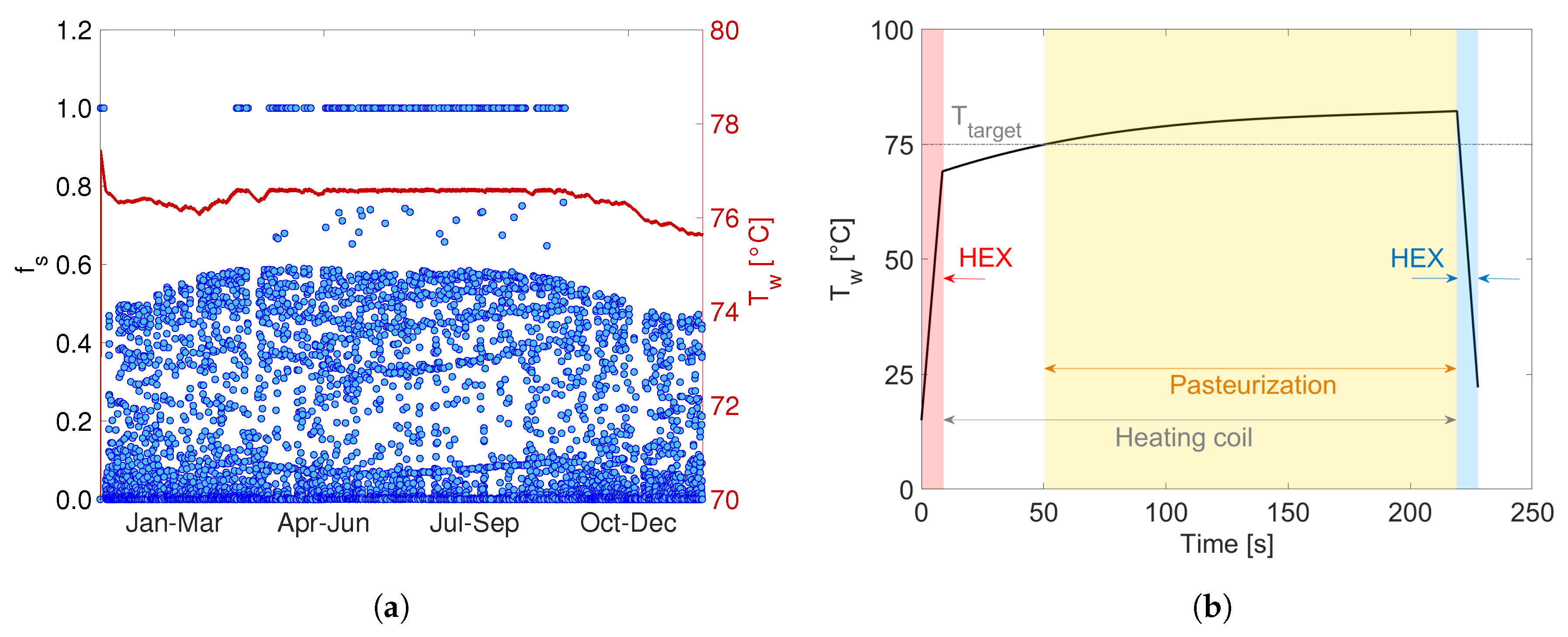
The shaft power required by the pumps depends on the mass-flow rate and on the total head losses as $P_p=\dot{m}gH/{\eta }_p$ (with ${\eta }_p$ being the efficiency of the pump). The total head has been evaluated as [42]

$$H=\gamma \left(\frac{{\dot{m}}^2}{d^n}\right)L,$$

(16)

with $\gamma =0.00164+0.000042/d$ being the friction factor, d the inner tube diameter, $n=5.08$ the exponent used for the considered pipes and L the total length of the piping, which is the sum of the physical length and the equivalent one. This last term, which takes into account the concentrated head losses, has been assumed equal to 10% of the real length [42]. The piping extension on the treatment line has been evaluated considering the whole length of the heating coils.

The pump for the solar field has been sized considering the length of the piping within the solar collectors. The solar collectors manufacturer suggests a minimum value for the mass flow rate of ${\dot{m}}_0=0.6$ L m${}^{-2}$ min${}^{-1}$ in order to avoid an excessively overheating of the aqueous coolant [31]. Starting from this value, the mass-flow rate in the solar field can be evaluated as ${\dot{m}}_{sf}={\dot{m}}_0{A}_c{N}_c$, being $A_c$ the cross-sectional area of the collector and $N_c$ the number of collectors. The pump is activated only if two conditions are met, namely the solar radiation is present and the temperature of the storage system is below an upper threshold (95 ${}^{\circ }$C). This latter condition is important to prevent the thermal storage temperature from exceeding the maximum value. The pump for the gas burner, on the other hand, is activated to provide the required mass-flow rate to the burner only if the temperature of the storage system is below a lower threshold (85 ${}^{\circ }$C).

The heat dissipated from the piping has been calculated iteratively starting from the data sheet provided by the manufacturer, in which the thermal losses per unit length are listed as a function of the pipe diameter.

3.6. Treatment Unit

The main treatment unit consists of a hot water storage tank which accommodates the heating coil employed for pasteurization purposes. Given that the solar irradiance varies during the day while the thermal power required for the water treatment is constant, the unit is designed to also serve as a thermal energy storage system for the excess solar thermal energy. The energy balance for this unit yields the thermal power available for pasteurization ${\Phi }_w$ as

$${\Phi }_{sf,u}+{\Phi }_{gb,u}={\left(\frac{d{E}_{i,tank}}{dt}\right)}_{tu}+{\Phi }_{hl,tu}+{\Phi }_w,$$

(17)

where

$$\begin{array}{cc}\hfill {\Phi }_{sf,u}=& {\eta }_{sf,pipe}{\epsilon }_{sf,coil}{\Phi }_{sf}\hfill \end{array}$$

(18)

$$\begin{array}{cc}\hfill {\Phi }_{gb,u}=& {\eta }_{gb,pipe}{\epsilon }_{gb,coil}{\Phi }_{gb}\hfill \end{array}$$

(19)

are respectively the useful heat power from the solar field and auxiliary gas burner, which are reduced by the thermal losses from the pipe lines through the efficiency ${\eta }_{pipe}$ and by the heat exchange efficiency ${\epsilon }_{coil}$ of the coils. The time-derivative of the internal energy $E_{i,tank}$ accounts for the heat storage in the tank (treatment unit). ${\Phi }_{hl,tu}$ quantifies the thermal losses from the tank towards the external environment, which are evaluated as

$${\Phi }_{hl,tu}=U{A}_{tank}({\overline{T}}_{tank}-T_{env}),$$

(20)

being U the overall thermal transmittance between the inner tank and the surrounding ambient, $A_{tank}$ the external surface of the tank, ${\overline{T}}_{tank}$ the mean temperature of water inside the tank and $T_{env}$ the environment temperature. Considering a tank made of concrete with a 100 mm thick rockwool layer insulation, the mean value of the thermal transmittance has been estimated as $U=0.31$ W m${}^{-2}$ K${}^{-1}$.

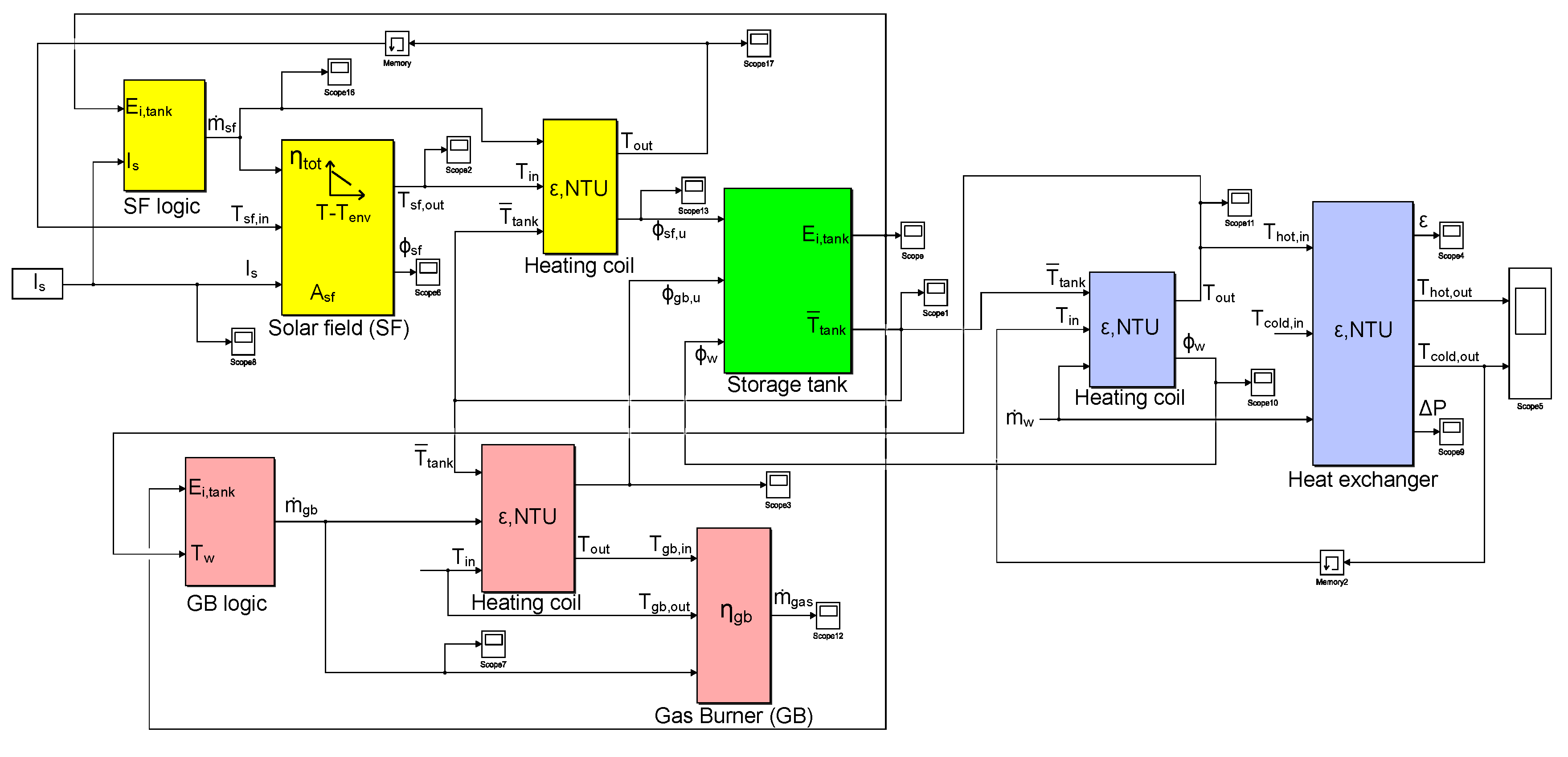
3.7. Lumped-Component Plant Model

A dedicated lumped-component model of the solar thermal water treatment plant has been developed in the Simulink${}^{\circledR }$ environment implementing the equations previously described, in order to simulate the performance of the plant during a whole year (see Figure 3 for an overview of the complete model). The model allows to evaluate the main operative parameters, such as temperatures, water flow rates and heat exchanged inside the various components using iterative procedures. In this study, four water treatment capacities have been investigated for the simulated plant, namely 50 L s${}^{-1}$ (i.e., 4320 m${}^3$ day${}^{-1}$), 100 L s${}^{-1}$ (i.e., 8640 m${}^3$ day${}^{-1}$), 250 L s${}^{-1}$ (i.e., 21,600 m${}^3$ day${}^{-1}$) and 500 L s${}^{-1}$ (i.e., 43,200 m${}^3$ day${}^{-1}$).

Figure 4a shows the contribution of the solar field with respect to the total thermal energy required for the water treatment in terms of the $f_s$ factor, which is defined as [43]

$$f_s={\Phi }_{sf}/({\Phi }_{sf}+{\Phi }_{gb}),$$

(21)

and the obtained treatment temperature during the year for the considered pasteurization protocol (114 s at 75 ${}^{\circ }$C). According to the design condition imposed, the treatment temperature is always above 75 ${}^{\circ }$C, and its nearly constant trend proves that the activation logic of the gas burner correctly provides the auxiliary thermal power to the thermal storage system when the solar field is not enough for driving the water pasteurization. In detail, the major contribution from the solar field is obtained during the summer period (i.e., approximately from May to September). Instead, during the winter period (from September to May), lower values in the available hourly solar irradiance for the chosen location of the plant (Torino, Italy) imply larger utilization of the gas burner, with a consequent higher value of the power provided by the natural gas usage and reduction of the $f_s$ factor. The wide distribution of the $f_s$ factor during the day would imply continuous switch-on/switch-off of the gas burner; however, the adopted system for thermal storage has been thought indeed to avoid this continuous transient operation of the gas burner.

On the other hand, Figure 4b shows the temperature of the treated water during its passage throughout the treatment line. First, the water temperature rises quickly in the plate heat exchanger during the pre-heating phase, from the ambient temperature to 70 ${}^{\circ }$C. The temperature is then further increased inside the treatment coil, where water is maintained above 75 ${}^{\circ }$C for about 170 s, to comply with the target pasteurization protocol. Finally, the treated water exits the circuit through the heat exchanger, where temperature drops to ambient conditions as heat is recovered and used to pre-heat the incoming raw water inflow.

4. Cost Estimation Model

The two parameters that are most commonly used to find the optimal configuration of solar thermal plants are the solar multiple and the thermal energy storage duration [44,45,46]. The solar multiple (SM) can be defined as the ratio between the effective aperture area of the collectors and that that would be required to obtain the target output power [44]. From its definition, it follows that SM > 1 represents an oversized solar field, while SM < 1 an undersized one. On the other hand, the thermal energy storage (TES) duration represents the time for which the storage system should be able to provide the required power without intervention of the primary energy sources (i.e., solar field or gas burner, in this case). Therefore, the heat storage system increases the flexibility of the plant. In the following sub-sections, we first detail the calculations of the different contributions to the total cost of the plant, and then discuss the possible plant optimization based on the previously mentioned parameters, namely the solar multiple and TES duration.

4.1. Capital Costs

The estimation of the capital cost for the simulated solar thermal pasteurization plant can be obtained using either the typical cost estimations methods available in the literature or the communicated costs from possible suppliers.

First, the cost analysis proposed by Turton et al. [47] has been considered for the costs of the tank, heating coils, pumps and gas burner. The overall installation cost, which includes direct and indirect expenses, for each component can be estimated as

$$C_{BM}=C_p^0\left(B_1+B_2{F}_M{F}_P\right)\frac{I_{2018}}{I_{2001}},$$

(22)

where $B_1$ and $B_2$ are coefficients depending on the type of component, while $F_M$ and $F_P$ are corrective factors related respectively to construction materials and operating pressure. While for the heating coils and pumps these parameters are provided separately (see

Table 1. Coefficients used for the capital cost evaluation of some components of the solar thermal pasteurization plant. Note that, for the tank and gas burner, $F_{BM}$ is directly provided [47].

Component	${\mathit{k}}_1$	${\mathit{k}}_2$	${\mathit{k}}_3$	${\mathit{B}}_1$	${\mathit{B}}_2$	${\mathit{F}}_{\mathit{P}}$	${\mathit{F}}_{\mathit{M}}$	${\mathit{F}}_{\mathbf{BM}}$
Tank	4.8509	−0.3973	0.1445	-	-	-	-	1.10
Heating coils	4.1884	−0.2503	0.1974	1.63	1.66	1.00	1.00	-
Pumps	3.3892	0.0536	0.1538	1.89	1.35	1.00	1.00	-
Gas burner	2.0829	0.9074	−0.0243	-	-	-	-	2.19

), the cost of the tank and gas burner is given as a function of $F_{BM}=B_1+B_2{F}_M{F}_P$. The ratio $I_{2018}/I_{2001}$ is used to take into account the changing value of money over time, and allows to estimate the current capital expenses using the purchase cost curves valid for a reference year (i.e., 2001 in this case [47]). The values $I_{2018}$ and $I_{2001}$ are obtained based on the chemical engineering plant cost index (CEPCI) of 567.5 (for 2018) and 397 for the reference year. The base cost $C_p^0$ of each component has been evaluated as

$$log{C}_p^0=k_1+k_{2}logA+k_3{\left(logA\right)}^2,$$

(23)

where $k_1$, $k_2$ and $k_3$ are factors depending on the equipment type, while A is a parameter related to the size of the component (see Table 1).

Second, the cost of the solar field has been considered equal to 335 EUR m${}^{-2}$, as provided by the manufacturer (Sky Pro 18 Advanced CPC, by Kloben Industries). The unit price of the plate heat exchanger, instead, has been considered to range from 506 EUR m${}^{-2}$ to 230 EUR m${}^{-2}$ depending on the considered size of the plant, as indicated by a possible supplier (T25-BFG, by Alfa Laval).

Figure 5 shows the contribution of the different components to the overall capital cost of a plant with 250 L s${}^{-1}$ capacity and different solar multiples (SM = 0.5, SM = 1.0, SM = 2.0 and SM = 3.0). In all the four cases, the duration of the thermal energy storage has been considered equal to 12 h. The most expensive component of the facility is found to be the solar field, which contributes for a percentage between 49.3% and 85.2% to the total capital cost. Other important contributions to the total cost are represented by the thermal storage system and gas burner, while the economizer and pumps account for a minor share.

4.2. Operating Costs

The operating costs of the plant are given by the sum of the expenses related to natural gas (auxiliary gas burner) and electricity (pumps) consumption. Here, these operating costs are estimated as

$$C_{op}=c_{ng}{M}_{ng}+c_{el}{E}_{el},$$

(24)

where $c_{ng}$ and $c_{el}$ are respectively the unit cost of natural gas and electricity, $M_{ng}$ is the gas consumption and $E_{el}$ the electrical energy’s one. Regarding electricity consumption, the primary water recirculating pumps, the one of solar field and the boiler’s pumping groups have been considered. The operating costs have been estimated using the results of the simulations with the considered pasteurization protocol, with energy prices taken from Eurostat database [48].

4.3. Insurance and Maintenance Costs

The maintenance $C_{main}$ and insurance $C_{ins}$ costs are due to the work and materials required for fixing breakdowns and by insurance contracts, respectively. Pitz-Paal et al. [49] investigated a large number of facilities, providing an accurate assessment of the maintenance costs, which can be considered equal to 1.5–2.0% of the capital expenses. In the last years, more recent studies [44,45,50] proved that this value has decreased, and it is now often between $0.5\%$ and $1.5\%$, in most cases not even exceeding $1.0\%$. In this work, a value of $1.0\%$ has been assumed.

4.4. Total Costs

The assessment of the optimal configuration and operation of the plant is based on the yearly running costs, which can be obtained as

$$C_{tot}=C_{op}+C_{main}+C_{ins}+C_{dep}.$$

(25)

In the equation above, the total cost depends on the operating costs $C_{op}$, maintenance costs $C_{main}$ and insurance costs $C_{ins}$ discussed in the previous sections, and on the depreciation $C_{dep}$ of the plant, which accounts for the loss of value of the facility over time. The depreciation can be expressed as a percentage of the capital cost, using the Capital Recovery Factor [47]

$$C_{dep}=C_{BM}\frac{{(1+i)}^{n}i}{{(1+i)}^n-1}.$$

(26)

Here the interest rate i has been evaluated using the Weighted Average Cost of Capital (WACC) as [51]

$$i=WACC=K_d\frac{D}{D+E}+K_e\frac{E}{D+E},$$

(27)

where E and D represent respectively the equity and the debt of the investment.

In Equation (27), $K_d$ is the cost of debt, which is evaluated as

$$K_d=IRS+spread,$$

(28)

being IRS (Interest Rate Swap) assumed equal to the Euribor index, namely $IRS=-0.27\%$ [48]. A value of $0.54\%$ has been considered for the spread [52]. The cost of equity, instead, can be written as:

$$K_e=R_{fr}+\beta EMRP.$$

(29)

The parameter $R_{fr}$ represents the return on a free risk investment (e.g., government bond) which, in the first semester of 2018, was set to $2.30\%$ [53]. The EMRP, which is the Equity Market Risk Premium, in the same period was equal to $6.10\%$ [53]. Finally, $\beta$ is a coefficient related both to the risk of company’s asset and to its strength, which takes into account how changes in the stock market have impact on society’s performance. This parameter has been assumed equal to $0.73$ [52]. From the calculations, a value of $6.99\%$ has been obtained for the $K_e$, while $K_d$ has been assessed to be $0.27\%$.

4.5. Economic Optimization Scenarios

Using the lumped-component model of the plant implemented in Simulink${}^{\circledR }$, an evaluation of the natural gas and electricity consumption during the years has been carried out for different combinations of solar multiple and TES duration (see

Table 2. Overview of the explored parameters for the plant configuration.

Parameter	Range	Units
Plant water treatment capacity	50 ÷ 500	L s${}^{-1}$
Solar Multiple (SM) of the plant	0 ÷ 3	-
Thermal Energy Storage (TES) duration	0 ÷ 12	hours

for an overview of the explored parameters for the plant configuration). In all the analyzed scenarios, a pasteurization temperature of $75{}^{\circ }$C and an expected lifetime of the plant equal to 20 years have been considered. The unit cost of water purification (expressed as EUR-cent m${}^{-3}$) obtained is shown in Figure 6: four different capacities of the plant have been analyzed, namely (a) 50 L s${}^{-1}$, (b) 100 L s${}^{-1}$, (c) 250 L s${}^{-1}$ and (d) 500 L s${}^{-1}$. In these calculations a 30% equity to 70% debt (i.e., $WACC=2.02\%$) mix has been considered, and the prices of the natural gas and electricity (including taxes) have been taken from Ref. [48]. The optimal configuration is found for 12 hTES duration in all the considered cases; whereas, the optimal solar multiple varies depending on the size of the plant (see also Figure 7a). The minimum cost among all the explored cases has been found to be ≈ 25 EUR-cent m${}^{-3}$, and is obtained for the 500 L s${}^{-1}$ plant and SM = 0.75. In general, when the solar field is oversized, an increase of the TES duration allows to reduce the costs of water purification. Note that the reduction of the water treatment cost with increasing sizes of the thermal storage system is generally more effective close to the optimal value of the solar multiple.

Clearly, the expected lifetime of the facility is an important parameter for assessing the depreciation rates. It is generally assumed that the useful life of a solar system is comprised between 20 and 30 years [44,45,54]. However, it is important to note that a plant is not only subject to physical degradation, but can also be replaced for different reasons, such as technical or commercial obsolescence. In fact, considering the development of new or unconventional technologies for water purification, the facility might be supplanted before the planned schedule. An analysis of the effect of lifetime on the 250 L s${}^{-1}$ plant is shown in Figure 7b, where the unit cost of water purification is reported for lifetimes between 10 and 30 years (the optimal duration of the thermal energy storage is considered, that is 12 h in all cases). As the figure shows, the unit costs of water treatment rises as the lifetime of the facility decreases, since the depreciation rates become higher. In addition, for a useful lifetime equal or lower than 10 years, the curve of unit cost does not present a minimum for any SM, meaning that the most convenient solution is to carry out the treatment without the solar system. On the other hand, if the useful lifetime is higher than 15 years, the solar system allows to reduce the unit cost, and the most advantageous size is increasingly larger (from $\mathrm{SM}=1.00$ when the lifetime is 15 years, to $\mathrm{SM}=1.75$ when the useful lifetime is 30 years).

5. Conclusions

A techno-economic analysis of a solar thermal plant for water pasteurization has been presented. The effectiveness of different thermal treatments was first evaluated experimentally, and one has been chosen as a test case for the development of a lumped-component model of the whole plant. The model has been shown to correctly guarantee the target treatment conditions, and then used to evaluate the performance of the plant in different configurations. The optimal plant configuration from a techno-economic perspective has been assessed on the basis of two design variables, namely the solar multiple and the thermal energy storage duration.

The most advantageous configuration has been obtained using a solar multiple between $0.75$ and $2.75$, according to the size of the plant, and a TES duration equal to 12 h. The unit cost of water treatment ranges from ≈32 EUR-cents m${}^{-3}$ for a 50 L s${}^{-1}$ facility, to ≈25 EUR-cents m${}^{-3}$ for a 500 L s${}^{-1}$ one.

Based on the reported analysis, it can be concluded that: (i) an increase of the thermal energy storage duration generally leads to reduction of costs; (ii) the optimal solar multiple depends on the considered scenario; (iii) the economic optimization model is very sensitive to the capital expenses. Indeed, the solar field represents the higher contribution to the capital cost; therefore, in perspective, the opportunity to access to the fiscal advantages for energy reclassification operations may be interesting to reduce the overall expenses. Starting from these latter general rules obtained for the four analysed cases, further up-scaling can be considered to assess the validity of these model predictions to even larger plant layouts.

Finally, other solar technologies may be also considered for the solar field; it would be indeed interesting to analyse the exploitation of, e.g., concentrated solar power. In addition, other renewable sources of heat or waste-heat recovery from industrial processes may be investigated to power the water treatment line [23,55,56].

References

1. WHO/UNICEF. Progress on Drinking Water, Sanitation, and Hygiene: 2017 Update and SDG Baselines; World Health Organization: Geneva, Switzerland, 2017. [Google Scholar]
2. Guidelines for Drinking-Water Quality, 4th ed.; World Health Organization (WHO) Chron.: Geneva, Switzerland, 2011; Volume 38, pp. 104–108.
3. Cheremisinoff, N.; Knovel, F. Handbook of Water and Wastewater Treatment Technologies; Chemical Petrochemical & Process; Elsevier Science: Amsterdam, The Netherlands, 2002. [Google Scholar]
4. Schwarzenbach, R.P.; Escher, B.I.; Fenner, K.; Hofstetter, T.B.; Johnson, C.A.; Von Gunten, U.; Wehrli, B. The challenge of micropollutants in aquatic systems. Science 2006, 313, 1072–1077. [Google Scholar] [CrossRef]
5. Bergamasco, L.; Alberghini, M.; Fasano, M. Nano-metering of solvated biomolecules or nanoparticles from water self-diffusivity in bio-inspired nanopores. Nanoscale Res. Lett. 2019, 14, 336. [Google Scholar] [CrossRef]
6. Howe, K.J.; Hand, D.W.; Crittenden, J.C.; Trussell, R.R.; Tchobanoglous, G. Principles of Water Treatment; John Wiley & Sons: Hoboken, NJ, USA, 2012. [Google Scholar]
7. Woldemariam, D.; Martin, A.; Santarelli, M. Exergy analysis of air-gap membrane distillation systems for water purification applications. Appl. Sci. 2017, 7, 301. [Google Scholar] [CrossRef] [Green Version]
8. Saber, O.; Kotb, H.M. Designing Dual-Function Nanostructures for Water Purification in Sunlight. Appl. Sci. 2020, 10, 1786. [Google Scholar] [CrossRef] [Green Version]
9. Lau, M.; Monis, P.; Ryan, G.; Salveson, A.; Blackbeard, J.; Gray, S.; Sanciolo, P. Selection of surrogate pathogens and process indicator organisms for pasteurisation of municipal wastewater—A survey of literature data on heat inactivation of pathogens. Process Saf. Environ. Prot. 2019, 133, 301–314. [Google Scholar] [CrossRef]
10. Voukkali, I.; Zorpas, A. Disinfection methods and by-products formation. Desalin. Water Treat. 2015, 56, 1150–1161. [Google Scholar] [CrossRef]
11. Hua, G.; Reckhow, D.A. Comparison of disinfection byproduct formation from chlorine and alternative disinfectants. Water Res. 2007, 41, 1667–1678. [Google Scholar] [CrossRef]
12. Von Gunten, U. Ozonation of drinking water: Part I. Oxidation kinetics and product formation. Water Res. 2003, 37, 1443–1467. [Google Scholar] [CrossRef]
13. Von Gunten, U. Ozonation of drinking water: Part II. Disinfection and by-product formation in presence of bromide, iodide or chlorine. Water Res. 2003, 37, 1469–1487. [Google Scholar] [CrossRef]
14. Hijnen, W.; Beerendonk, E.; Medema, G.J. Inactivation credit of UV radiation for viruses, bacteria and protozoan (oo) cysts in water: A review. Water Res. 2006, 40, 3–22. [Google Scholar] [CrossRef]
15. Gray, N.F. Ultraviolet Disinfection. In Microbiology of Waterborne Diseases; Elsevier: Amsterdam, The Netherlands, 2014; pp. 617–630. [Google Scholar]
16. Nguyen, H.T.; Corry, J.E.; Miles, C.A. Heat resistance and mechanism of heat inactivation in thermophilic campylobacters. Appl. Environ. Microbiol. 2006, 72, 908–913. [Google Scholar] [CrossRef] [PubMed] [Green Version]
17. Lindahl, T. Irreversible heat inactivation of transfer ribonucleic acids. J. Biol. Chem. 1967, 242, 1970–1973. [Google Scholar] [PubMed]
18. Verma, S.K.; Singhal, P.; Chauhan, D.S. A synergistic evaluation on application of solar-thermal energy in water purification: Current scenario and future prospects. Energy Convers. Manag. 2019, 180, 372–390. [Google Scholar] [CrossRef]
19. Chiavazzo, E.; Morciano, M.; Viglino, F.; Fasano, M.; Asinari, P. Passive solar high-yield seawater desalination by modular and low-cost distillation. Nat. Sustain. 2018, 1, 763–772. [Google Scholar] [CrossRef] [Green Version]
20. Hohne, P.; Kusakana, K.; Numbi, B. A review of water heating technologies: An application to the South African context. Energy Rep. 2019, 5, 1–19. [Google Scholar] [CrossRef]
21. Zhou, L.; Li, X.; Ni, G.W.; Zhu, S.; Zhu, J. The revival of thermal utilization from the Sun: Interfacial solar vapor generation. Natl. Sci. Rev. 2019, 6, 562–578. [Google Scholar] [CrossRef] [Green Version]
22. Signorato, F.; Morciano, M.; Bergamasco, L.; Fasano, M.; Asinari, P. Exergy analysis of solar desalination systems based on passive multi-effect membrane distillation. Energy Rep. 2020, 6, 445–454. [Google Scholar] [CrossRef]
23. Morciano, M.; Fasano, M.; Bergamasco, L.; Albiero, A.; Curzio, M.L.; Asinari, P.; Chiavazzo, E. Sustainable freshwater production using passive membrane distillation and waste heat recovery from portable generator sets. Appl. Energy 2020, 258, 114086. [Google Scholar] [CrossRef]
24. Fasano, M.; Bergamasco, L.; Lombardo, A.; Zanini, M.; Chiavazzo, E.; Asinari, P. Water/Ethanol and 13X Zeolite Pairs for Long-Term Thermal Energy Storage at Ambient Pressure. Front. Energy Res. 2019, 7, 148. [Google Scholar] [CrossRef] [Green Version]
25. Verrilli, F.; Srinivasan, S.; Gambino, G.; Canelli, M.; Himanka, M.; Del Vecchio, C.; Sasso, M.; Glielmo, L. Model predictive control-based optimal operations of district heating system with thermal energy storage and flexible loads. IEEE Trans. Autom. Sci. Eng. 2016, 14, 547–557. [Google Scholar] [CrossRef]
26. Pizzolato, A.; Donato, F.; Verda, V.; Santarelli, M.; Sciacovelli, A. CSP plants with thermocline thermal energy storage and integrated steam generator–Techno-economic modeling and design optimization. Energy 2017, 139, 231–246. [Google Scholar] [CrossRef]
27. Feachem, R.G.; Bradley, D.J.; Garelick, H.; Mara, D.D. Sanitation and Disease: Health Aspects of Excreta and Wastewater Management; John Wiley and Sons: Hoboken, NJ, USA, 1983. [Google Scholar]
28. Alberghini, M.; Morciano, M.; Bergamasco, L.; Fasano, M.; Lavagna, L.; Humbert, G.; Sani, E.; Pavese, M.; Chiavazzo, E.; Asinari, P. Coffee-based colloids for direct solar absorption. Sci. Rep. 2019, 9, 4701. [Google Scholar] [CrossRef]
29. Alexander, M. Most probable number method for microbial populations. Methods Soil Anal. Part 2 Chem. Microbiol. Prop. 1983, 9, 815–820. [Google Scholar]
30. Lazzarin, R.; Noro, M.; Righetti, G.; Mancin, S. Application of hybrid PCM thermal energy storages with and without al foams in solar heating/cooling and ground source absorption heat pump plant: An energy and economic analysis. Appl. Sci. 2019, 9, 1007. [Google Scholar] [CrossRef] [Green Version]
31. Kloben Industries S.r.l. Scheda Tecnica: Collettore Solare Sky Pro Advanced; Kloben Industries S.r.l.: Milano, Italy, 2016. [Google Scholar]
32. PVGIS: Photovoltaic Geographical Information System. Available online: http://re.jrc.ec.europa.eu/pvgis/ (accessed on 18 September 2018).
33. Marcel, S.; Huld, T.; Dunlop, E. PV-GIS: A web-based solar radiation database for the calculation of PV potential in Europe. Int. J. Sol. Energy 2005, 24, 55–67. [Google Scholar]
34. Moore, N.; Gibson, N.; Wright, G. Hot water service using high-efficiency gas-fired appliances. Build. Serv. Eng. Res. Technol. 1992, 13, 147–153. [Google Scholar] [CrossRef]
35. Roslyakov, P.; Proskurin, Y.V.; Ionkin, I. Increase of efficiency and reliability of liquid fuel combustion in small-sized boilers. J. Phys. Conf. Ser. 2017, 891, 012243. [Google Scholar] [CrossRef]
36. Bergman, T.L.; Incropera, F.P.; DeWitt, D.P.; Lavine, A.S. Fundamentals of Heat and Mass Transfer; John Wiley & Sons: Hoboken, NJ, USA, 2011. [Google Scholar]
37. Khan, T.; Khan, M.; Chyu, M.; Ayub, Z. Experimental investigation of single phase convective heat transfer coefficient in a corrugated plate heat exchanger for multiple plate configurations. Appl. Therm. Eng. 2010, 30, 1058–1065. [Google Scholar] [CrossRef]
38. Neagu, A.; Koncsag, C.; Barbulescu, A.; Botez, E. Estimation of pressure drop in gasket plate heat exchangers. Ovidius Univ. Ann. Chem. 2016, 27, 62–72. [Google Scholar] [CrossRef] [Green Version]
39. Kakaç, S.; Liu, H.; Pramuanjaroenkij, A. Heat Exchangers: Selection, Rating, and Thermal Design, 2nd ed.; Taylor & Francis: Abingdon, UK, 2002. [Google Scholar]
40. Whitaker, S. Forced convection heat transfer correlations for flow in pipes, past flat plates, single cylinders, single spheres, and for flow in packed beds and tube bundles. AIChE J. 1972, 18, 361–371. [Google Scholar] [CrossRef]
41. Churchill, S.; Chu, H. Correlating equations for laminar and turbulent free convection from a horizontal cylinder. Int. J. Heat Mass Transf. 1975, 18, 1049–1053. [Google Scholar] [CrossRef]
42. Citrini, D.; Noseda, G. Idraulica; Casa Editrice Ambrosiana: Rozzano, Italy, 1987. [Google Scholar]
43. Duffie, J.A.; Beckman, W.A. Solar Engineering of Thermal Processes; John Wiley & Sons: Hoboken, NJ, USA, 2013. [Google Scholar]
44. Abrams, A.; Farzan, F.; Lahiri, S.; Masiello, R. Optimizing Concentrating Solar Power with Thermal Energy Storage Systems in California; DNV GL: Oslo, Norway, 2014. [Google Scholar]
45. González-Portillo, L.; Muñoz-Antón, J.; Martínez-Val, J. An analytical optimization of thermal energy storage for electricity cost reduction in solar thermal electric plants. Appl. Energy 2017, 185, 531–546. [Google Scholar] [CrossRef]
46. Guédez, R.; Spelling, J.; Laumert, B.; Fransson, T. Optimization of Thermal Energy Storage Integration Strategies for Peak Power Production by Concentrating Solar Power Plants. Energy Procedia 2014, 49, 1642–1651. [Google Scholar] [CrossRef] [Green Version]
47. Turton, R.; Bailie, R.C.; Whiting, W.B.; Shaeiwitz, J.A. Analysis, Synthesis and Design of Chemical Processes; Pearson Education: London, UK, 2008. [Google Scholar]
48. Eurostat Energy Database. Available online: https://ec.europa.eu/eurostat/web/energy/data/database (accessed on 12 November 2018).
49. Pitz-Paal, R.; Dersch, J.; Milow, B. European Concentrated Solar Thermal Road-Mapping; The German Aerospace Center (DLR): Stuttgart, Germany, 2005. [Google Scholar]
50. Taylor, M. Renewable Energy Technologies Cost Analysis Series: Concentrating Solar Power; IRENA: Abu Dhabi, United Arab Emirates, 2012; Volume 1. [Google Scholar]
51. Mellen, C.M.; Evans, F.C. Valuation for M & A: Building Value in Private Companies; John Wiley & Sons: Hoboken, NJ, USA, 2010; Volume 587. [Google Scholar]
52. Damodaran, A. Equity Risk Premiums (ERP): Determinants, Estimation and Implications—The 2019 Edition. Soc. Sci. Res. Netw. 2019. [Google Scholar] [CrossRef] [Green Version]
53. Fernandez, P.; Pershin, V.; Acin, I. Market Risk Premium and Risk-Free Rate used for 59 Countries in 2018: A Survey. Soc. Sci. Res. Netw. 2018. [Google Scholar] [CrossRef]
54. Izquierdo, S.; Montañés, C.; Dopazo, C.; Fueyo, N. Analysis of CSP plants for the definition of energy policies: The influence on electricity cost of solar multiples, capacity factors and energy storage. Energy Policy 2010, 38, 6215–6221. [Google Scholar] [CrossRef]
55. Morciano, M.; Fasano, M.; Secreto, M.; Jamolov, U.; Chiavazzo, E.; Asinari, P. Installation of a concentrated solar power system for the thermal needs of buildings or industrial processes. Energy Procedia 2016, 101, 956–963. [Google Scholar] [CrossRef] [Green Version]
56. Schwantes, R.; Cipollina, A.; Gross, F.; Koschikowski, J.; Pfeifle, D.; Rolletschek, M.; Subiela, V. Membrane distillation: Solar and waste heat driven demonstration plants for desalination. Desalination 2013, 323, 93–106. [Google Scholar] [CrossRef] [Green Version]
Sample Availability: Specific or different uses of the above reported quantities are detailed in the text.
Figure 1. (Left) Overview of the equipment for the experimental tests: (1) aluminum test tubes and tailor-made 3D-printed holder (detail of the CAD drawing in the inset); (2) thermostatic water bath (CORIO CD-300F, Julabo); (3) industrial furnace for thermostatic applications (TypeM120-VF, MPM Instruments); (4) laptop for data acquisition; (5) digital hot plate stirrer (AREX Digital, VELP Scientifica) for sanitation of the test tubes after each test. (Right) Temperature of the samples during the disinfection tests for the four considered pasteurization protocols, namely 540 s at 70 C, 114 s at 75 C, 30 s at 80 C and 8 s at 85 C. The solid lines show the mean temperature obtained for each pasteurization protocol (four repetitions each), while the related transparent bands the range between the minimum and maximum values.
Applsci 10 04771 g001
Figure 2. Overview of the plant layout, which consists of: a solar field for primary solar thermal energy collection; an auxiliary gas burner to overcome the intermittent nature of the solar resource; a central treatment unit for the pasteurization, which also serves as heat storage system; a plate heat exchanger for waste-heat recovery and pre-heating of the water to be treated.
Applsci 10 04771 g002
Figure 3. Overview of the Simulink ® lumped- model of the solar pasteurization plant. Solar field, gas burner, heat exchanger and storage tank subsystems are identified with yellow, red, blue and green, respectively.
Applsci 10 04771 g003
Figure 4. Results of the numerical model: (a) f s factor (blue dots) and treatment temperature (red solid line); (b) mean temperature of the water to be treated during its passage throughout the plant. The red and blue sections highlight respectively the pre-heating and post-cooling of the fluid through the plate heat exchanger, which acts as an economizer. The results refer to the 250 L s 1 plant capacity.
Applsci 10 04771 g004
Figure 5. Components percentage values on the facility cost for various SM values: (a) S M = 0.5 ; (b) S M = 1.0 ; (c) S M = 2.0 ; (d) S M = 3.0 . The duration of the thermal energy storage has been considered equal to 12 h, the capacity of the plant equal to 250 L s 1 .
Applsci 10 04771 g005
Figure 6. Unit cost of water pasteurization (expressed as EUR-cent per cubic meter of treated water) as a function of the solar multiple and thermal energy storage duration for different treatment capacities of the plant: (a) 50 L s 1 ; (b) 100 L s 1 ; (c) 250 L s 1 ; (d) 500 L s 1 . Calculations consider 20 years as expected plant lifetime.
Applsci 10 04771 g006
Figure 7. Unit cost of water pasteurization as a function of the solar multiple for (a) different capacities of the plant (20 years lifetime) and (b) different expected lifetime of the plant (250 L s 1 ). All these calculations consider 12 h of thermal energy storage duration.
Applsci 10 04771 g007