1. Introduction
The use of technology in education is getting more and more intensive day by day, and it is becoming a necessity for effective and permanent learning to be updated. Technology has been utilized and continues to be used in many areas such as students’ access to course materials, administrators’ follow-up management processes, teachers’ course control, and activities in education. Particularly in the field of Artificial Intelligence (AI), the technology has moved effectively in education to a different dimension with a significant leap [
1]. It is well-known that students benefit not only in material access, but also in monitoring their processes, evaluating their learning, and monitoring their performance, through intelligent tutoring systems (ITS). One of these ITS is developed in the LIS (Learning Intelligent System) project [
2], which aims to assist students in their educational processes. LIS is a system formed within the Universitat Oberta de Catalunya (UOC) to develop an adaptive system to be globally applicable at the custom Learning Management System (LMS) implemented at UOC to help students to succeed in their learning process. The project intends to provide help to the student in terms of automatic feedback in assessment activities, recommendations in terms of learning paths, self-regulation or learning resources, and gamification techniques to improve the students’ engagement.
The first stage of this project focuses on the development of an Early Warning System (EWS) to detect at-risk students by using data from the past and present and to warn the student and his or her teacher about the situation. Also, the system provides semi-automatic feedback as an early intervention mechanism in order to amend possible conditions of failure. A proof of concept of the EWS was proposed in [
3], where sound results in terms of a predictive model and the application of the EWS in a higher education course were presented. Such experiment was used as a pillar to build a functional and enhanced version of the EWS at the UOC where the learning process is held by a custom LMS.
This paper aims at presenting a new system with several contributions. The first contribution is a predictive model denoted as Gradual At-Risk (GAR) model. Such a model is based only on students’ grades and predicts the likelihood to fail a course. A deep analysis of the model is performed in the whole set of courses at the university by using the data available in a data mart provided by our institution. Compared to [
3], we propose a method to obtain the best classifier and training set for each course and semester. This method was proposed after observing that new data do not always contribute to improving the accuracy and, therefore, sometimes should be discarded.
The second one is a method to determine a threshold to consider the trained GAR model of a course as a high- or low-quality model. The GAR model, when used in a real educational setting, will provide to the student feedback based on her/his risk level. Therefore, a teacher cannot afford to send a wrong message or recommendation to the student. This threshold is used for the EWS to adapt the type of message sent to the student.
The third contribution is the application of the EWS in a real educational setting in two courses. The GAR model is used to provide meaningful information to the students and teachers in terms of dashboards and feedback. In this paper, we analyze the accuracy of identifying at-risk students in such a real learning scenario and the impact on the final performance of the courses. We consider also relevant this last contribution, since it proves the application of the AI in the educational field. These contributions are drawn as a consequence of answering the next research questions underpinning this study:
RQ1. How accurate is the predictive model in the whole institution after six semesters of available data?
RQ2. Which is the accuracy limit for the predictive model to consider a low-quality model to adapt the intervention measures in the EWS?
RQ3. How accurate is the EWS in identifying at-risk students in a real educational setting?
The paper is organized as follows.
Section 2 summarizes related work and
Section 3 focuses on the methods and context of the institution where the research took place.
Section 4 analyzes the process to obtain the best classification algorithm and training set for the GAR model, and
Section 5 presents two of the main dashboards provided by the EWS as well as the implemented feedback intervention mechanism. The experimental results on two case studies are described in
Section 6, while
Section 7 discusses the results. Finally, the conclusions and future work are summarized in
Section 8.
2. Related Work
2.1. Predictive Models
As described in different systematic reviews [
4,
5], many models can be applied to education. Students’ performance [
6], students’ dropout within an individual course [
7,
8], program retention [
9], recommender systems in terms of activities [
10], learning resources, [
11] and next courses to be enrolled [
12,
13] are some examples of the application of those models.
Independently of the desired outcome, models have used many different types of data in order to perform the predictions. Different variables (or features) have been explored ranging from demographic data [
14] (e.g., age, gender, ethnic origin, marital status, among others), self-reported questionnaires [
15,
16], continuous assessment results [
17,
18], user-generated content [
19] to LMS data [
20,
21].
Numerous classification algorithms have been analyzed through the proposed predictive models. Decision Tree (DT) [
22], Naive Bayes (NB) [
23], Support Vector Machine (SVM) [
24], Logistic Regression [
25,
26,
27], Hierarchical Mixed models [
17,
28], K-Nearest Neighbors (KNN) [
26], Neural Network models [
29], or Bayesian Additive Regressive Trees [
30] are some examples of the employed techniques.
As previously mentioned, we focus on identifying at-risk students by checking the likelihood to fail a course following the claims of other researchers [
24,
25,
31] to create specific course predictive models. A simple model based on grades of the continuous assessment activities (named GAR model) is used instead of using a complex model. Activities performed by students throughout their learning process are indicators of the performance they will reach in the future. Although we use this simple model, we have comparable results with other predictive models to detect at-risk students.
Table 1 illustrates a comparison of the predictive GAR model with other related works where more complex models were proposed. The table shows for each comparison, the intervention point in the semester timeline (
Semester Intervention Point), the compared accuracy metric (
Accuracy Metric), the value of the metric in the referenced work (
Value Metric Ref.), the LOESS regression of the GAR model at the intervention point in the complete set of courses at our university (
LOESS Regr. GAR whole institution), and the percentages of courses with a metric value larger than the metric of the referenced work (
Perc. Courses Metric GAR > Metric Ref.). Authors in [
23] obtained an F
1,5 (F-score) of 62.00% with Naive Bayes at 40% of the semester timeline; meanwhile, our model reaches a LOESS regression value of 78.55% on average in the whole courses at our university at the same point of the semester timeline. When courses are evaluated individually, we found that more than 70% of the courses have an F
1,5 larger than 62.00% at this point of the semester. Authors in [
25] reached a TNR (True Negative Rate) of 75.40% at the end of the course meanwhile the GAR model reaches a LOESS regression value of 97.56%, and more than 99% of the courses have a TNR larger than 75.40%. Authors in [
30] computed the MAE (Mean Absolute Error) at 40% of the semester timeline. They reached a MAE value of 0.07, whereas the GAR model has a LOESS value of 0.08, and more than 64% of the courses have a MAE smaller than 0.07 at this point of the semester. The approach presented in [
32] reached a TPR (True Positive Rate) of 81.00% at the 40% of the semester timeline while our model obtained a LOESS regression value of 80.46% but more than 40% of the courses have a TPR larger than 81.00% at this point of the semester. On the approach presented in [
33], where SMOTE was used in order to balance classes, the AUC (Area Under The Curve) ROC (Receiver Operating Characteristics) curve was used to evaluate the model. The best model reached a ROC value near to 91.00% at 60% of the semester timeline. The GAR model without SMOTE has a LOESS value near to 93.00% and more than 59% of the courses have a ROC value larger than 91.00% at this point of the semester.
2.2. Early Warning Systems
An EWS is a tool used to monitor students’ progress. It identifies students at-risk of either failing or dropping out of a course or program [
23]. It helps students to be on track and aid in their self-directed learning journey [
34]. Also, it can help to reach the necessary information about student engagement and performance to facilitate personalized timely interventions [
28].
Based on the predictive models mentioned in the previous section, some examples of EWS are students’ dropout detection on face-to-face environments [
35], students’ dropout on online settings [
36,
37,
38], or early identification of at-risk students, which may allow some type of intervention to increase retention and success rate [
16,
25,
26,
39].
Many of the previously described approaches propose an EWS, but the EWS is just sketched from a conceptual point of view. Therefore, few full-fledged developments can be found. The most referenced one is the Course Signals at Purdue University [
17] where different dashboards are available at the student’s and teacher’s point of view. Moreover, the system triggers a visual warning alert using a Green-Amber-Red semaphore. Other systems can be found where information is available in dashboards for teachers [
31,
40,
41] and students [
42].
Personalized feedback [
17] is one possible intervention mechanism for these kind of approaches. Other intervention mechanisms can be applied, such as pedagogical recommendations [
43], mentoring [
44], or academic support environment [
45], with a significant impact on performance, dropout, and retention. Feeding students depending on his or her situation will affect students’ perception and will impact his or her way of learning and self-regulation. If personalized feedback can be one of the possible intervention mechanisms, nudges can complement it in a very constructive way. Nudges according to the definition provided in [
46] (p. 2) are “interventions that preserve freedom of choice that nonetheless influence people’s decisions”. Nudges have their origin in behavioral economics, which studies the effects of psychological knowledge about human behavior to enhance decision-making processes. In education [
47], nudges intend to obtain a higher educational attainment (e.g., improvement of grades, to increase course completion rates and earned credits, or to increase course engagement and participation), and they have been used in primary, secondary, and higher education, including Massive Open Online Courses (MOOC), and involving different stakeholders (parents, students, and teachers). The information provided by nudges includes remainders, deadlines, goal setting, advice, etc. How the information included in nudges is stated can also increase social belonging and motivation.
The EWS we propose is able to provide personalized feedback. First, students receive predictions from the first activity about the minimum grade they should obtain in the activity to succeed in the course prior to the submission deadline date. Thus, the student is knowledgeable about the effort he or she should apply in the activity to have a chance to pass the course. This prediction is updated after each graded activity and a new prediction is generated for the next one. This type of prediction differs from other approaches where the models can only be used after a certain number of activities, denoted as the best point of intervention when enough data have been gathered to have an accurate model. Second, the teacher can complement these predictions with constructive feedback from the very beginning of the course, including recommendations to revert (or even prevent) at-risk situations.
3. Methods and Context
3.1. University Description: Educational and Assessment Model
The UOC from its origins (1995) was conceived as a purely online university that used the Information and Communication Technologies (ICT) intensively for both the teaching-learning process and management. This implies that most of the interactions between students, teachers, and administrative staff occur within the UOC’s own LMS, generating a massive amount of data. Its educational model is centered on the students and the competences they should acquire across their courses. The assessment model is based on continuous assessment and personal feedback is given to students after obtaining a mark when delivering assessment activities. Thus, any student enrolled is having a personalized learning process by means of quantitative, but also qualitative feedback. Although the student profile is aged up to the regular ones with family and full job employed, they devote time to learn in order to get a better position in their job or to enhance their knowledge with another bachelor’s degree. Students at UOC are really competence oriented, but usually, they lack daily time for all personal and professional tasks. This student background and their profiles became a cornerstone to developing the EWS to guide them in a personal way when being assessed and when receiving personal feedback.
The assessment process within a course is based on a continuous assessment model combined with summative assessment at the end of the semester. Therefore, there are different assessment activities during the semester and a face-to-face final examination at the end of the course. The final mark is computed based on a predefined formula for each course where each assessment activity has a different weight depending on the significance of the assessment activity contents within the course. The UOC grading system is based on qualitative scores on assessment activities. Each assessment activity is graded with the following scale: A (very high), B (high), C+ (sufficient), C- (low), D (very low), where a grade of C- and D means failing the assessment activity. In addition, another grade (N, non-submitted) is used when a student does not submit the assessment activity. Also, UOC courses are identified by codes, and students are randomly distributed in classrooms. Finally, the semesters are coded by academic year and the number of the semester (i.e., 1 for fall and 2 for spring semester). For instance, 20172 identifies the 2018 spring semester of the academic period 2017/2018.
3.2. Data Source: The UOC Data Mart
The UOC provides their researchers and practitioners with data to promote a culture of data evidence-based decision-making. This approach is materialized in a centralized learning analytics database: the UOC data mart [
48]. The UOC data mart collects and aggregates data that are transferred from the different operational data sources using ETL (Extract-Transform-Load) processes, solving problems as data fragmentation, duplication, and the use of different identifiers and non-standardized vocabularies for describing the same real-world entities. During the ETL processes, sensitive data are anonymized (personal data are obfuscated, and all internal identifiers are changed to a new one [
49]).
UOC uses from its origins a custom LMS [
50] that has been improved and upgraded several times during the last 25 years (the current version is version 5.0) according to the new requirements of learners, teachers, and available technology. Although the campus has a high interoperability to add external tools (e.g., Wordpress, Moodle, MediaWiki, among others), mainly the learning process is done in the custom classrooms. Operational data sources include data from the custom LMS and other learning spaces (e.g., data about navigation, interaction, and communication), as well as data from institutional warehouse systems (CRM, ERP, etc.), which include data about enrollment, accreditation, assessment, and student curriculum, among others. As a result, the UOC data mart offers: (1) historical data from previous semesters; (2) data generated during the current semester aggregated by day. Currently, the UOC data mart stores curated data since the academic year 2016–2017.
3.3. Gradual At-Risk Model
A GAR model is built for each course, and it is composed of a set of predictive models defined as submodels based only on a student’s grades during the assessment process. A course has a submodel for each assessment activity, and each submodel uses the grades of the current and previous graded assessment activities as features to produce the prediction. Note that, there is no submodel for the final exam since there is nothing to produce a prediction from when the final score of the course can be computed straightforwardly from the complete set of grades (i.e., the assessment activities and the final exam) by using the final mark formula.
The prediction outcome for the submodels is to fail the course. This is a binary variable with two possible values: pass or fail. We are interested in predicting whether a student has chances to fail the course, and we denote this casuistic as at-risk student. Although a global at-risk prediction taking into account all enrolled courses is an interesting outcome, we focus individually on each course to give simple messages and recommendations to the student on courses in which she or he is at-risk.
Example 1. Let us describe the GAR model for a course with four Assessment Activities (AA). In such a case, the GAR model contains four submodels:
PrAA1(Fail?) = (GradeAA1)
PrAA2(Fail?) = (GradeAA1, GradeAA2)
PrAA3(Fail?) = (GradeAA1, GradeAA2, GradeAA3)
PrAA4(Fail?) = (GradeAA1, GradeAA2, GradeAA3, GradeAA4)
where PrAAn(Fail?) denotes the name of the submodel to predict whether the student will fail the course after the assessment activity AAn. Each submodel PrAAn(Fail?) uses the grades (GradeAA1, GradeAA2,…, GradeAAn), that is, the grades from the first activity until the activity AAn. Each submodel can be evaluated based on different accuracy metrics. We use four metrics [23]:where TP denotes the number of at-risk students correctly identified, TN the number of non-at-risk students correctly identified, FP the number of at-risk students not correctly identified, and FN the number of non-at-risk students not correctly identified. These four metrics are used for evaluating the global accuracy of the model (ACC), the accuracy when detecting at-risk students (true positive rate—TPR), the accuracy when distinguishing non-at-risk students (true negative rate—TNR) and a harmonic mean of the true positive value (precision) and the TPR (recall) that weights correct at-risk identification (F score - F1,5). Note that, the area under the ROC curve (AUC) is not considered on this study [51]. 3.4. Next Activity At-Risk Simulation
The GAR model only provides information about whether the student has the chance to fail the course based on the last graded assessment activities. This model can be used to give information to the student about the likelihood to fail, but it is not very useful when the teacher wants to provide early and personalized feedback concerning the next assessment activities. We define the Next Activity At-risk (NAAR) simulation as the simulation to determine the minimum grade that the student has to obtain in the next assessment activity to have a chance to pass the course.
This prediction is performed by using the submodel of the assessment activity we want to predict. The NAAR simulation uses the grades of the previous activities already graded and simulates all possible grades for the activity we want to predict for identifying when the prediction changes from failing to pass.
Example 2. Let us take the submodel PrAA1(Fail?) of Example 1. In order to know the minimum grade, six simulations are performed based on the possible grades the student can obtain in AA1. Each simulation will produce an output based on the chances to fail the course. An output example is shown next based on the first assessment activity of the Computer Fundamentals course that will be analyzed in Section 6.| PrAA1(Fail?) = (N) | → | Fail? = Yes |
| PrAA1(Fail?) = (D) | → | Fail? = Yes |
| PrAA1(Fail?) = (C-) | → | Fail? = Yes |
| PrAA1(Fail?) = (C+) | → | Fail? = Yes |
| PrAA1(Fail?) = (B) | → | Fail? = No |
| PrAA1(Fail?) = (A) | → | Fail? = No |
where we can observe that students have a high probability of passing the course when they get a B or an A grade on the first assessment activity. This means that most of the students pass when they obtain these grades. However, it is possible to pass the course with a lower mark, but less frequently. Note that, this is for the first assessment activity where there are no previous activities. On further activities, the grades of previous activities are taken into account and the prediction is better personalized for each student based on his or her previous grades. 3.5. Datasets
Table 2 describes the datasets used for each semester. As we can observe, the number of registries for training increases each semester that are counted from the 2016 fall semester (20161). This number depends on the number of enrolled students. The number of offered courses also differs on each semester and depends on the opened and extinguished academic programs in the semester taken as testing semester, and a minimum number of ten enrollments per course to open the course stated by the university.
3.6. Generation and Evaluation of the Predictive Model
The GAR model is built by using Python and the machine learning Scikit-Learn library [
52], while the statistical analysis has been performed by the analytical tool R [
53]. The GAR model for a given course is trained based on the historical data of previous semesters from the 2016 fall semester (i.e., 20161), and the test is performed on the data of the last historical available semester from the UOC data mart (that is hosted in Amazon S3). For example, for semester 20171, the models are trained with data from semesters 20161 and 20162 to test it on the semester 20171. During the validation test, four algorithms are tested: NB, DT, KNN, SVM.
In order to evaluate the classification algorithms, the GAR model is built for each course of the institution based on the number of assessment activities (see Example 1 in
Section 3.3). Each course has a different number of assessment activities and some courses have a final exam. In such cases, the submodel for the final exam is not generated since the final grade can be straightforwardly computed from all grades of the assessment activities and the final exam, and no prediction is needed. Then, the training and test are performed for each course and submodel. In order to analyze the results globally for the whole institution, the value of each metric described in
Section 3.3 is ordered and uniformly distributed among the semester timeline based on the submission date of the respective assessment activity associated with the submodel. For instance, for a course with four assessment activities, the prediction of the first assessment activity is set to the position at 20%, the second at 40%, the third at 60%, and the fourth at 80% of the semester timeline. Note that, this distribution changes on courses with a different number of activities. This distribution helps to identify at each stage of the timeline the average quality of the GAR model based on the submitted assessment activities at that time for the whole institution. Finally, in order to evaluate the different classification algorithms, the LOESS regression [
54] is used. Although a linear regression would show a pretty linear perception of the increment of the accuracy, this would not represent the correct relationship between metrics and timeline. The LOESS regression shows a better approximation due to the large number of values.
The NB was selected in [
3] as the best classification algorithm to be used in the institution based on the performance observed on the four metrics. Precisely, the selection was mainly done by the results of the TPR and F
1,5 since these metrics tend to indicate the algorithm that mostly detects at-risk students.
Currently, we have more data in the data mart, and further analysis can be done on how it is evolving the GAR model among the semesters. Specifically, three more semesters can be analyzed (i.e., until 2019 spring semester). We can answer the research questions RQ1 and RQ2 by (1) analyzing how the NB performance evolves during these three semesters; (2) proposing a method to obtain the best classification algorithm and training set for each assessment activity and course; and, finally, (3) determining a method to deduce a threshold to consider the GAR model of a course as a high- or low-quality model.
During the semester, trained models are used by means of an operation that is run on the daily information available at the UOC data mart. A cron-like Python script downloads the data from the UOC data mart and checks whether students have been graded for any assessment activity proposed in the course. When this happens, the corresponding NAAR simulation is executed by getting the respective trained GAR model. All these functionalities (e.g., train, test, statistical analysis, and daily predictions) among others are embedded into the EWS. The full description of the technical architecture and capabilities of the EWS can be found in [
55].
3.7. Case Studies in Real Educational Settings
The GAR model and the EWS that hosts it have been tested through pilots in two real learning scenarios, as will be presented in
Section 6, because LIS project follows a mixed research methodology that combines an action research methodology with a design and creation approach. This mixed research methodology as well as the outputs it produces are depicted in
Figure 1.
Action research methodology allows to investigate and improve own practices, guided by the next principles [
56]: concentration on practical issues, an iterative cycle plan-act-reflect, an emphasis on change, collaboration with practitioners, multiple data generation methods, and finally, action outcomes plus research outcomes and research.
The design and creation approach is especially suited when developing new Information Technology (IT) artifacts. It is a problem-solving approach that uses an iterative process involving five steps [
57]: Awareness (the recognition of a problem where actors identify areas for further work looking at findings in other disciplines); Suggestion (a creative leap from curiosity about the problem offering very tentative ideas of how the problem might be addressed); Development (where the idea is implemented, depending on the kind of the proposed IT artifact); Evaluation (examines the developed IT artifact and looks for an evaluation of its worth and deviations from expectations); and Conclusion (where the results of the design process are consolidated and the gained knowledge is identified).
First, the problem to solve (learners’ at-risk identification) is detected and shared by teachers and educational institutions. Secondly, a solution (the EWS) is suggested. Thirdly, the EWS is implemented and proved in different real learning scenarios following the iterative cycle of plan-act-reflect. This cycle is done through pilots conducted across courses during several academic semesters by cycles. At the end of each cycle, an evaluation process is done. This will probably cause changes and improvements in the EWS, and the initiation of a new cycle until a final artifact is available and ready to be used in educational institutions.
4. Algorithms and Training Dataset Selection for the GAR Model
4.1. Naive Bayes Evaluation
In order to evaluate the NB algorithm, we used the datasets described in
Section 3.5 and the evaluation process described in
Section 3.6 for the four semesters from the 2017 fall semester (20171) to the 2019 spring semester (20182). The results processed with R-based scripts are shown in
Figure 2 and
Table A1 in
Appendix A for the four metrics ACC, TNR, TPR, and F-score 1,5 with a LOESS regression.
In general, we can observe that adding more training data helps to improve all the metrics with respect to the baseline 20171. However, the last two semesters (i.e., 20181 and 20182) do not impact on getting better TPR results, i.e., correctly detect at-risk students. This is due to mostly the students at UOC tending to pass the courses. The average performance rate in the institution was 78.90% in the 2018/2019 academic year [
58]. Thus, more data help to identify new situations when students are not at-risk, and new data have a low impact on detecting new at-risk students.
4.2. Algorithm and Training Set Selection
As mentioned previously, we observed that the metrics do not always improve over semesters for specific courses, even though more training data are available. Different factors may impact on these results: 1) The behavior of students in some semesters may add noise to the model that produces worse results; or 2) some academic change such as new resources or changes in the difficulty or the design of the assessment activities may impact the grades of a specific semester. In order to deal with these issues, we propose a method to select the best training set and classification algorithm for each course and activity. This selection can be reduced to an optimization problem with the objective function
L to be maximized
where
STR is the semester to explore as training set,
STE is the semester to perform the validation test,
M is the classification algorithm used to perform the training, and
DS,C,A is a slice from the whole dataset
D based on the semester
S, course
C and activity
A. After different tests, we found that the best choice is to maximize the sum of the TPR and TNR. This function tends to select classifiers and training sets that achieve good results in both metrics, while maximizing one of the metrics tends to penalize the discarded one.
The method has been split into two algorithms. The first algorithm selects the best classification algorithm, while the second one selects the best training set for each assessment activity of each course. The selection of the best algorithm (see Algorithm 1) searches for the best algorithm based on four available classification algorithms: NB, DT, KNN, and SVM. The process is quite simple but computationally expensive since four training processes are run for each course and assessment activity. However, there is a substantial benefit since each activity (i.e., each submodel for the GAR model associated with the course) has the best-selected algorithm.
| Algorithm 1. Pseudocode of Best_Classification_Algorithm. |
| Input: STR: Semester training dataset, STE: Semester test dataset |
| Output: BCL: Best Classification Algorithm per course and activity |
| Steps: |
| Initialize(BCL) |
| For each course C ϵ STE do |
| For each activity A ϵ C do |
| MCL← Select best classifier M ϵ {NB, KNN, DT, SVM} based on opt. function L(STR, M) (Equation (2)) |
| BCL(C, A, STR) ← {STR, MCL} |
| |
| Return BCL |
The second process is presented in Algorithm 2. In this case, the process goes further, and it explores for the submodel of the activity the surrounding submodels in terms of previous activities within the same course, and the same submodel within the same course in the previous semesters. We observed that sometimes an activity is not mandatory, or it has a low impact on the final grade of the course, or a semester adds noise to the model, and such a semester produces a lower accurate submodel. For example, it is commonly observed in our institution that the behavior of the students is different depending on the spring or fall semester. Thus, in such cases, we suggest selecting the best-known training set within the same course in previous activities or in the same activity among previous semesters. Note that the computational cost is even higher than the former since the evaluation test should be redone with the training set of the selected semester and the test set of last available semester. We are aware that this process will be unfeasible when the number of semesters increases. Thus, a window of training semesters should be defined in the future.
| Algorithm 2. Pseudocode of Best_Classification_and_Training_Set. |
| Input: STE: Semester test dataset |
| Output: BCL: Best classification algorithm and training set per course and activity |
| Steps: |
| //Train and test all semesters with respect to STE |
| BCL ← ∅ |
| For each semester S ϵ {20171, …, STE} do |
| BCL ← BCL ∪ Best_Classification_ Algorithm (S, STE) |
| |
| //Compare on same semester |
| For each semester S ϵ {20171, …, STE} do |
| For each course C ϵ S do |
| For each pair (Ai, Aj) ϵ C st. i < j do |
| {S, MAi} ← BCL(C, Ai, S) |
| {S, MAj} ← BCL(C, Aj, S) |
| If L(S, MAi) > L(S, MAj) then BCL(C, Aj, S) ← {S, MAi} |
| |
| //Compare inter semester |
| For each course C ϵ STE do |
| For each activity A ϵ C do |
| For each pair (S, STE) st. S ϵ {20171, …, STE-1} |
| {S, MS} ← BCL(C, A, S) |
| {STE, MSTE} ← BCL(C, A, STE) |
| If L(S, MS) > L(STE, MSTE) then BCL(C, A, STE) ← {S, MS} |
| |
| Return BCL |
In order to analyze the performance of these two algorithms, the evaluation test has been performed only in the last semester 20182 for the different metrics and taking as a baseline the NB classifier results. The results are shown in
Figure 3 and
Table A2 in
Appendix A. The best algorithm selection slightly improves the different metrics since the best selection is only performed within the explored algorithms on an activity. In the case of the TPR, the LOESS regression compared to the NB improves from the range 44.60–86.04% to 47.88–88.43%. However, considerable improvement is obtained with the second algorithm, where the LOESS regression increases until 58.79–93.60%. This result will help to define a more significant threshold to consider a high-quality submodel, as we will see in the next section.
Although the last finding proves that the second process helps to identify the best classifier and training set for each assessment activity, it is not clear which classifier has been mostly selected and from which origin semester.
Table 3 summarizes this information with interesting insights. The table shows the percentage of classifiers and from which semester they have been selected. The process mostly selected the DT with more than half of the trained submodels.
The NB proposed in [
3] is only selected the 25.92% of the total. Thus, we conclude that the NB is not the most appropriate classifier to train the models when more data are available. Finally, we can observe that the distribution among semesters is quite reasonable. The training dataset of the last available semester is the most selected one (36.69%), but for some submodels, the dataset from previous semesters with less training data helps to get more accurate models. Finally, we give an insight about the computational cost of this operation in absolute numbers for semester 20182. The number of training operations for each semester are 26,468 in 20182, 24,996 in 20181, 23,144 in 20172 and 24,184 in 20171. Note that, this number for a semester takes into account the training operation for the four classifiers for all courses and activities.
4.3. Quality Threshold Identification
Some predictive models aimed at early identify at-risk students defined the best point of intervention during the semester. This point is deduced from the experimental results [
23] or is fixed before the evaluation [
59]. Our EWS performs interventions from the first assessment activity. Thus, the concept of intervention point has nonsense. In our system, the submodels (i.e., the training model applied on each assessment activity) are classified based on high- or low-quality models based on the TPR and TNR since the intervention measures are adapted based on the quality of the model. For instance, an intervention action based on a likelihood to fail the course cannot be applied as-it-is when the submodel has a low-quality TPR.
Similarly, a praise message based on a likelihood to pass cannot be applied when the submodel has a low-quality TNR. In those cases, the interventions are adapted when the likelihood to fail or pass cannot be assured (see
Section 5 for further details). This classification is performed based on a quality threshold that can be defined globally for the institution or individually for each course based on the teacher’s experience.
In this section, we seek the quality threshold globally applicable to demonstrate that the GAR model can be valid with a unique threshold for the whole institution and avoid particular cases. Also, we want to analyze whether the method presented in Algorithm 2 to obtain the best algorithm classifier and training set can improve this threshold with respect to [
3] where the threshold selection was performed by observation without any data analysis.
The quality threshold identification can be reduced to an optimization problem since the objective is to maximize the threshold while the number of submodels considered high-quality do not worsen significantly. However, this problem is unfeasible to be solved because there is no optimal solution. Thus, we define a function to be maximized in order to approximate the problem
where
x is the threshold value,
positions of the semester timeline,
wi is a weight that can be assigned to the position
i of the semester timeline, and
Si is the set of all the submodels that the submission deadline is in the position
i. In summary, the function seeks to sum the threshold value with the weighted average of the number of submodels that their TPR is above the threshold for each position of the semester timeline. We defined a weighted average due to it might being interesting to give more relevancy to some positions of the semester. Note that, we assume in our optimization problem all positions with the same weight (i.e.,
wi = 1). Moreover, the TPR is used since we are interested to particularly maximize the threshold over submodels for detecting at-risk students.
After solving the optimization problem for the 2019 spring semester with an R-based script, the result is illustrated in
Figure 4a where
f(x) summands are plotted in the axis. As we can observe, both summands generate a curve of Pareto Points with the optimum on the threshold 75% (i.e., the function
f(x) maximized on the threshold 75%). Thus, we define high-quality submodels as all submodels with a TPR higher than 75%.
In order to further compare with [
3], we computed the percentage of explored courses where the TPR and TNR are higher than thresholds 70% and 75% (see
Figure 4b). Note that, we removed the multiple plots for the TNR because there was only an average increment of 1–3% over each threshold. For the 2019 spring semester, even increasing the threshold to 75%, we obtain better coverage of high-quality submodels compared to the 2017 fall semester, where the threshold was set to 70%. The coverage is quite similar for the TNR at 25% from 70.07% of the courses to 69.80% but there is a considerable increment at 50% from 89.31% to 97.12%. Although only 26.71% of the courses will have a TPR higher than 75% at 25% of the semester timeline (it was 24.01% on 2017 fall semester), this value increases considerably to 74.58% at the 50% of the semester timeline (it was 65.95% in 2017 fall semester).
5. The Early Warning System: Dashboards and Feedback Intervention Mechanism
The EWS provides data visualization features to teachers and students by means of dashboards. Those features are complemented with a feedback intervention mechanism. The full description of the technical architecture and capabilities of the EWS can be found in [
55].
Students and teachers have different dashboards and permissions. Students have a simple dashboard to see the prediction to succeed in the enrolled courses. The prediction is based on the NAAR simulation, and a Green-Amber-Red semaphore (similar to [
17]) that warns the students about their warning classification level. A semaphore in green represents that the student is non-at-risk, while a semaphore with a red signal indicates a high likelihood to fail. For an assessment activity, the student gets first the prediction of the minimum grade that she or he should obtain to have a high likelihood to pass the course. This prediction is received while the student is working in the assessment activity (see
Figure 5a). When the assessment activity is submitted and assessed, the grade (see the triangles above and below the C- grade in the bar corresponding to the first assessment activity in
Figure 5b) and the warning level are updated in the student dashboard, and the prediction for the next assessment activity (the second assessment activity in the case of
Figure 5b) is computed and plotted in the dashboard as a new bar.
Teachers have a different dashboard to see the performance of the students and help them in case of trouble.
Figure 6 shows a tabular dashboard where all the students of a course are shown. As we can observe, only students who have consented to participate in the study (by signing a consent form) can be reviewed. For those who accepted, the teacher can easily check the progress of the predictions and warning levels. The readability is quite clear based on the same Green-Amber-Red semaphore used for the students. Teachers have a new color classification (the black color) to detect potential students’ dropout (i.e., students that do not submit their assessment activities).
The EWS is able to provide feedback messages as an early intervention mechanism. Feedback messages contain recommendations, and also nudge students, especially those being at-risk [
60]. The intervention mechanism is implemented by means of a feedback messaging system that aims to enhance teachers’ actions over students depending on their status, thus providing a better understanding about their own learning process. From the teacher’s point of view, the system forces them to provide early and personalized feedback to students when delivering each assessment activity. From the students’ point of view, the EWS is providing them the teacher feedback, but also a probabilistic percentage of their success. It is also providing students with richer and valuable information: what they have to do in order to improve their learning process and obtain a better grade and pass the course. They are also simultaneously nudged to better perform the next activity (the importance of the activity on the upcoming activities is provided, as well as the provision of additional learning resources) and the importance for better planning. In summary and according to [
47], the information provided in the feedback messages contains nudges that fall in the categories of goal setting, informational nudges, assistance, and reminders.
Figure 7 summarizes in a decision tree the rationale behind the EWS concerning the students’ warning level when an assessment activity is graded, which in turn, impacts the feedback message to be sent. When graded, a feedback message is triggered to each student for notifying his or her warning level (predictive statement), as well as the feedback for the next assessment activities. The system distinguishes different situations depending on the warning level, and the feedback message is adapted depending on the specific situation. Green (G) means that the student is not at-risk when the TNR is greater than the minimum threshold of 75% established in
Section 4.3 (i.e., the model is considered a high-quality model). In such a case the student receives a comforting message in order to congratulate him or her. Yellow (or amber) means that the student is not considered at-risk, but he or she can be in the near future. The feedback message alerts the student about his or her chances to pass and gives some recommendations to progress successfully in the course. In addition, the feedback message also contains explanations about the accuracy of the prediction because, in some cases, the prediction (may pass or may fail) is under the quality threshold. Therefore, information about the TNR and TPR constitutes one of the differences among the three different types of yellow messages (Y1, Y2, and Y3) that are sent in this case. The distinction of different situations in yellow messages constitutes an enhancement regarding the work presented in [
3], where no such distinction existed. This is especially relevant in the case of students that, in spite of passing the assessment activity, the grade obtained is under the grade suggested by the predictive model (message Y2). Red and black represent that the student is at serious risk of failing or dropping out (at-risk student). When the student has submitted and failed the assessment activity, (R) is the most critical situation, although the effort of submitting the activity is positively valued by the teachers. In this case, the feedback message contains recommendations to get out of this situation. Also, the message suggests the student contact his or her teacher in order to talk about the difficulties the student is experiencing in the course. Potentially, this can derive in a more individual support. The case when the student has not submitted the last or the last two assessment activities (B1 and B2) is dealt separately from the previous case, representing a potential dropout student. The feedback message asks for the reasons for not submitting the activities and reminds the student of his or her options to pass the course (information about mandatory assessment activities and the final exam). Unfortunately, and depending on the timeline of the semester, the student can receive a feedback message confirming him or her that has hopelessly failed the course. In such a case, the student receives advice to avoid this situation the next time he or she enrolls in the course, and the proposal of tasks the student can perform before a new semester starts.
From an educational point of view, the EWS is a powerful tool to reduce dropout and increase students’ engagement. It is providing a constructive answer for not disappointing students. In the case of students that are not properly following the course, the system is pointing out how they can improve by showing them new opportunities and even the mandatory assessment activities remaining to successfully pass the course. Finally, students that have not submitted their assessment activities can provide very useful information to the teacher, not only to build better feedback messages for the next edition of the course but also to introduce enhancements in the next course editions (new learning resources, better course design, etc.).
6. Case Studies: Computer Fundamentals and Databases
The EWS has been tested in two case studies to answer the research question RQ3. The EWS aims to detect but also support at-risk students, which basically means, to help them to continue their learning process by providing accurate and valuable feedback for not failing or dropping out.
Specifically, the EWS has been introduced in Computer Fundamentals and Databases courses. Both courses are online courses offered in the Computer Science bachelor’s degree and in Telecommunication bachelor’s degree at UOC. While Computer Fundamentals is a first-semester course, Databases is offered in the fourth one. Thus, students’ knowledge and expertise are quite different when performing each one. Both courses are 6 ECTS and their assessment model is based on continuous assessment (several assessment activities are proposed along the semester, some of them are practical activities that imply the development of artifacts) and a final face-to-face exam at the end of the semester.
In Computer Fundamentals (a first-year course), students are devoted to learning the main principles for designing digital circuits and the basis of the computer architecture. In Databases, students are devoted to learning what databases are (and the specialized software that manages them), and how to create and manipulate relational databases using the SQL language (both interactive and embedded SQL). For the Databases course, previous knowledge is required (in programming and logic), so this is the reason to be in the fourth semester. The Computer Fundamentals course has a high number of students enrolled each semester (between 500–600 students) and becomes the first contact with the custom LMS. The Databases course has over 300 students each semester, but students already know very well the UOC educational model as well as how the LMS works. So, they are not as new in Databases as they are in Computer Fundamentals. Thus, both courses are excellent ones to evaluate the EWS and analyze whether at-risk students can be correctly identified and help them through the early feedback system. The system has been tested in both courses during one semester. Previously, a proof of concept was also tested as it can be seen in [
3], but now a new version of the EWS is tested with new features and enhancements suggested by teachers and students when collecting their perception, as explained in [
60]. As mentioned in
Section 3.7, this process has been done following the design and creation research method that uses an iterative model to better develop IT artifacts to solve real problems. This new version of the EWS is the second iteration.
The EWS was tested during the first semester of the academic course 2019/2020 (i.e., 20191 semester). A total of 313 students from Computer Fundamentals (CF) gave their consent to test the system, and a total of 71 students from Databases (DB) gave it too. To sum up, 384 students were testing it. In both courses, and after teachers graded each assessment activity, the EWS was triggering predictions to students, as well as personalized feedback messages, which depended on the warning level classification of the students presented in
Section 5. According to the numbers of students taking part in the pilot, and the number of assessment activities performed, the system triggered 1607 predictions (CF: 1252; DB: 355). Feedback messages attached to each prediction and assessment activity were previously designed and analyzed by teachers, with the aim of motivating students for further assessment activities. Feedback messages tended to be as personalized as the system allowed, and they included some nudges to support the students learning process according to their grades.
The quantitative analysis provided below compares both courses involved in the case studies, according to the following criteria: assessment model and performance of GAR model, the performance of the system for correctly classifying students according to their warning level and the statistical significance on the final mark distribution as a consequence of the use of the EWS.
6.1. Performance of GAR Model
CF course has four assessment activities starting during the semester timeline at 0% (AA1), 25% (AA2), 50% (AA3) and 75% (AA4) approximately. The formula to compute the final mark (FM) is:
where
GradeAAn is the grade of the assessment activity AAn and
GradeEXAM is the grade of the final exam. The AA4 (which is a practical assessment activity) and the EXAM are mandatory, and they have a significant impact on the final score. Note that, the course can be even passed without performing the three first activities. However, the teachers know by experience that it is difficult to pass the course without the first three activities where fundamental topics are learnt. Thus, most of the students pass the course by completing the four activities.
In the case of DB course, five assessment activities are delivered during the semester timeline at 0% (AA1), 20% (AA2), 40% (AA3), 60% (AA4), and 80% (AA5), approximately. AA2, AA3, and AA5 are practical activities that deal with SQL concepts (basic SQL statements, triggers, and stored procedures, and JDBC, respectively). The final mark (FM) in the DB course is computed as follows. First, a global mark for the practical assessment activities (Grade
P) is computed. In case the student delivers AA2, AA3, and AA5, the two best grades are selected, and Grade
P is computed as the average of both grades. Otherwise, the average of the two submitted practical activities is the global mark for the practical assessment activities. Secondly, the final mark for the course (FM) is:
Students must perform at least two of three practical activities (AA2, AA3, and AA5) and the final exam (EXAM) in order to pass the course. Although AA1 and AA2 are optional, most of the students pass the course by completing these optional activities too, similarly to CF.
Table 4 shows the performance of the GAR model for both courses. For each submodel,
TP, FP, TN, FN, and the accuracy metrics
ACC, TNR, TPR, and
F1,5 are summarized. The table also shows the best algorithm (
Algorithm) and the last semester for the training set (
Semester) that was used to train each submodel (as detailed in
Section 4.2). Although, in the case of CF the first submodel (which corresponds to the AA1) is considered a low-quality model for detecting non-at-risk students (i.e., TNR smaller than the threshold of 75%), the quality is good for the rest. In the case of DB, the accuracy is very good from the very beginning of the course in the detection of the students that are likely to pass the course (TNR begins at 89.53%). That means that the grade for AA1 is a very good indicator to predict success in DB. However, the submodel still does not predict correctly students that may fail the course (TPR is 68.18%). This fact is very different in the CF course, where the students at-risk are detected from the AA1 (TPR 82.83%).
6.2. Performance of the Warning Level Classification
Regarding the accuracy of the warning level classification, the results for each assessment activity are shown in
Table 5 for both courses. On the one hand, the table shows the number of students assigned to each classification level (
No.) and the final performance of the students for each warning level (
Fail, Pass). The set of messages to be sent according to the warning level classification (
WL) has been previously discussed in
Section 5 (see
Figure 7). The final performance for each case gives insights about the correct assignation of the students.
As it can be observed, in the case of CF and for the AA1, students were mostly assigned to the yellow warning level. This was due to the low-quality of the submodel, and it is consistent with the results previously discussed (see
Table 5). In subsequent assessment activities, all the colors were used. It is worth noting that the accuracy improved, and students assigned to the yellow color were those students that passed the assessment activity, but with a grade lower than the grade suggested by the prediction. The green color was correctly assigned for 74.5% of the students, and the red and black (non-submitted) to 93.5% and 100%, respectively on AA2. Similar results were observed in the AA3 and the AA4. Some students assigned to red color in the AA2 moved to black in the upcoming assessment activities because they did not submit previous activities, causing course dropout. The yellow color only served as medium risk level at first assessment activities, whereas students were progressively moved to the respective correct risk level on the final ones.
Concerning the DB course, and on the contrary of CF, some students were assigned to the green color in AA1. This is consistent with the fact that the grade obtained in AA1 was a good indicator for predicting course success. A percentage of 78.2 of the students were correctly informed about their chances of success, and this ratio increased significantly in the upcoming assessment activities up to 89.8 and 93.6% in AA2 and AA3, respectively. This is consistent with the fact that AA2, AA3, and AA5 were (at least two of them) mandatory activities, and students prioritize the submission of AA2 and AA3 in order to accomplish this requirement as soon as possible in the course timeline. In fact, most of the students assigned to the green color delivered AA2, AA3, and AA5. Similar to CF, yellow color warned students that their performance was under the prediction in all the assessment activities. Students assigned to the red color appear in AA2 (first potentially mandatory assessment activity), and 73.3% were correctly identified at-risk, and this ratio increased until 80.0% in AA3. Clearer than in the case of CF, students assigned to red color in AA2 moved to black color in the subsequent assessment activities.
We also checked whether there is statistical significance on the final mark distribution comparing the semester where the case studies were run concerning the previous semester (20182, i.e., 2019 spring semester). The objective is to see whether the EWS has impacted the performance of the courses. We used the unpaired two-sample Wilcoxon test due to the non-normal distribution of the final mark [
61]. Here, we assume as the null hypothesis that the marks are worse or equal than in the previous semester. Note that, the dropout students are not taken into account. For CF, the p-value < 0.04 and, thus, we can reject the null hypothesis, the median of the final mark increases from 7.8 to 7.9, and the dropout decreases from 51% to 31% on the students who signed the consent. The results regarding retention and scoring are slightly better, but we cannot claim that they are only inferred from the utilization of the EWS, since difficulty on the activities may be different, and the percentages were computed based on students who signed. Those students are generally more engaged, and they tend to participate in pilots (i.e., self-selection bias).
Related to DB, the p-value < 0.02 and we can also reject the null hypothesis, the median of the final mark increases from 7 to 7.6, and the dropout decreases from 26 to 17%. A similar claim to CF can be done. However, the difference is significantly better. This course does not have the variability in terms of marks that a first-year course has. The students have already done several courses in an online learning setting. Therefore, they know better how to self-regulate to pass the course compared to new students of a first-year course that do not have this prior experience.
7. Discussion
In this section, we discuss the contributions proposed in this paper and we conclude the answers to the research questions. Related to RQ1 and RQ2, we provided a method to select the best algorithm classifier and training set for each assessment activity and course in order to always get one of the best submodels. The results presented in
Section 4.2 prove a high accuracy of the GAR predictive model when it is analyzed in the whole institution.
Focusing on RQ1 (How accurate is the predictive model in the whole institution after four semesters of available data?), the GAR model has improved significantly compared to the results presented in [
3], by increasing the size of the datasets and selecting the best algorithm and training set. As an example, the LOESS regression of the TPR improved on the NB of the 2017 fall semester from 38.96–77.69% until 58.79–93.60% of the optimal selection in the 2019 spring semester. The GAR model has comparable results to more complex models that take into account other features such as CGPA, enrolled semesters, attempted times, as stated in
Section 2.1.
There are still many courses where it is challenging to detect at-risk students in the first half of the semester since there is a low number of failing students. Although resampling methods for imbalance classes [
62,
63] can be applied, we need to analyze thoroughly if this model is suitable for these courses and maybe other models should be applied to guide the students. Also, the GAR model has a relevant limitation. When the assessment process is changed regarding the number of assessment activities or contents of the activities, the model is invalid for the course. Although other models presented in the literature are also affected by the same limitation [
17,
18], we solved the problem with the best selection process. In such cases, the method proposed in
Section 4.2 tends to select the previous best-known submodel (mostly the previous assessment activity) and such a trained submodel is applied. Even having nearly ten percent of courses (around 100 courses in the 2019 fall semester) with such changes in the assessment model, the results presented in such a section were unaffected. We observed that the behavior of the students is quite similar when only one assessment activity is changed but it starts to fail on major changes. In such limitations, we should consider new features as further research in order to improve the global accuracy of the system.
Related to RQ2 (Which is the accuracy limit for the predictive model to consider a low-quality model to adapt the intervention measures in the EWS?), we increased the intervention threshold to 75% without losing any high-accurate model in terms of TPR with a new method by transforming the search to an optimization problem. Thus, the intervention mechanism can provide more focused early feedback messages based on high accurate TPR and TNR.
Concerning RQ3 (How accurate is the EWS on identifying at-risk students in a real educational setting?), two case studies have been analyzed in order to answer this research question. The EWS is capable to correctly predict the likelihood to fail the course and the Green-Amber-Red risk classification is capable of classifying the risk level correctly in both case studies, even though the courses have different assessment models and the behavior and experience of the students are significantly different. In terms of performance and dropout, there is a slight improvement. However, we cannot assure that it is only based on the EWS utilization.
Related to the early feedback intervention mechanism, the EWS uses feedback messages nudging [
46], intervention [
64], and counseling [
42]. The classification of seven different conditions provides a high personalization. In a fully online setting, early feedback is one of the most appropriate mechanisms in terms of scalability. Also, we found that the feedback sent to the students based on their progress to their email accounts are highly appreciated by the students. These results are consistent with those exposed in [
47]. This feedback was part of the intervention mechanism discussed in [
60]. Furthermore, some students that were in at-risk situation decided to contact the teacher after receiving this early feedback in order to get additional educational support (i.e., 40 students in Computer Fundamentals and 12 students in Databases during all the semester).
In terms of the results of the case studies, there are some threats to validity to consider. In terms of internal validity, self-selection bias and mortality may affect the quantitative analysis. Students gave their consent to be included in the pilot since this is required in our institution by the Research Ethical Committee [
65]. Thus, engaged students tend to participate in such pilots, and performance computed on those students tends to be higher compared to the average of the course. However, it is worth noting that the teachers received replies to the early feedback on dropout students and nobody complained about the system, they congratulated the initiative and even some of them apologized for dropping out of the course and not reaching the course objectives.
8. Conclusions and Future Work
AI will be fundamental in the coming years for supporting education and develop new educational systems for supporting online learning. The ongoing pandemic pointed out the deficiencies that we currently have in education (on-site but also online) [
66] and the need to improve our learning processes and environments. Tools like those presented in this paper, but also others based on automatic recommendation [
67], are some examples of systems that could enhance the way the learning processes are currently done and leverage the work of the teachers on learning contexts with a large number of students.
In this paper, we have presented an EWS from the conceptualization of the predictive model to the complete design of the training and test system and a case study on a real setting. The predictive model has a high accuracy within individual courses, but it has still some deficiencies for identifying at-risk on the first assessment activities. As future piece of work, we are planning to extend the experiments in two directions. On the one hand, the bottleneck mentioned on selecting the most appropriate training set and classifier should be fixed. This process will be prohibitive in the next semesters due to the large exploration and a smarter method should be developed. Inserting a clustering process to detect regions of data with relevant information, applying SMOTE on courses with imbalanced data, or a vote ensemble approach could be different strategies to apply to improve quality and runtime. On the other hand, adding information about the profile of the students can help to better classify students based on their behavior at the institution. This new information can improve the accuracy of the predictions or even detecting students with different needs (i.e., newbie students, repeater students, etc.).
Related to the EWS, we are ready to further analyze the students’ behavior within courses in the sense that optimal learning paths can be discovered and proposed to students to improve their learning experience. Also, we plan to start analyzing the students’ behavior outside courses in order to check the successful set of enrollment courses within the same semester and discourage the enrollment of conflictive sets. In the end, the aim of the system will be the same: to help students to succeed in their learning process.
Author Contributions
Conceptualization, D.B., A.E.G.-R., and M.E.R.; methodology, A.E.G.-R. and M.E.R.; software, D.B.; validation, D.B., A.E.G.-R., M.E.R., and A.K.; formal analysis, D.B., A.E.G.-R., and M.E.R.; investigation, D.B., A.E.G.-R., M.E.R., and A.K.; data curation, D.B; writing—original draft preparation, D.B., A.E.G.-R., M.E.R., and A.K.; writing—review and editing, D.B., A.E.G.-R., M.E.R., and A.K.; visualization, D.B., A.E.G.-R., and M.E.R.; supervision, D.B., A.E.G.-R., M.E.R., and A.K.; project administration, D.B. and A.K. All authors have read and agreed to the published version of the manuscript.
Funding
This research has been funded by the eLearn Center at Universitat Oberta de Catalunya through the project New Goals 2018NG001 “LIS: Learning Intelligent System”.
Acknowledgments
The authors express their gratitude for the technical support received by the eLearn Center staff in charge of the UOC data mart.
Conflicts of Interest
The authors declare no conflict of interest.
Appendix A
Table A1.
LOESS Regression of the Naive Bayes in the complete set of courses in the different datasets.
Table A1.
LOESS Regression of the Naive Bayes in the complete set of courses in the different datasets.
| Semester Timeline | ACC | TNR | TPR | F1.5 |
|---|
| 20171 | 20172 | 2081 | 20182 | 20171 | 20172 | 2081 | 20182 | 20171 | 20172 | 2081 | 20182 | 20171 | 20172 | 2081 | 20182 |
|---|
| 10% | 75.98 | 78.51 | 80.43 | 80.59 | 90.15 | 89.14 | 90.62 | 91.39 | 38.97 | 47.03 | 43.59 | 44.14 | 39.90 | 47.44 | 45.03 | 46.54 |
| 15% | 77.42 | 80.19 | 81.79 | 82.58 | 91.24 | 89.14 | 90.59 | 92.02 | 44.21 | 52.44 | 48.28 | 49.14 | 44.99 | 52.12 | 48.75 | 51.03 |
| 20% | 78.78 | 81.72 | 83.09 | 84.33 | 92.08 | 89.25 | 90.66 | 92.54 | 49.04 | 57.42 | 52.83 | 53.93 | 49.65 | 56.52 | 52.52 | 55.37 |
| 25% | 80.02 | 83.07 | 84.31 | 85.82 | 92.70 | 89.39 | 90.81 | 92.94 | 53.43 | 61.98 | 57.23 | 58.51 | 53.84 | 60.60 | 56.30 | 59.51 |
| 30% | 81.13 | 84.27 | 85.45 | 87.12 | 93.14 | 89.57 | 91.03 | 93.26 | 57.39 | 66.11 | 61.40 | 62.79 | 57.57 | 64.32 | 59.97 | 63.39 |
| 35% | 82.11 | 85.27 | 86.46 | 88.15 | 93.31 | 89.78 | 91.30 | 93.43 | 60.91 | 69.74 | 65.37 | 66.85 | 60.82 | 67.68 | 63.59 | 67.07 |
| 40% | 83.06 | 86.22 | 87.45 | 89.00 | 93.47 | 90.21 | 91.71 | 93.62 | 63.98 | 72.88 | 69.03 | 70.49 | 63.68 | 70.70 | 67.07 | 70.42 |
| 45% | 83.57 | 87.11 | 88.54 | 89.81 | 93.68 | 90.62 | 92.26 | 93.93 | 66.39 | 75.87 | 72.51 | 73.73 | 65.89 | 73.42 | 70.42 | 73.39 |
| 50% | 84.12 | 87.83 | 89.49 | 90.64 | 93.89 | 90.85 | 92.75 | 94.31 | 68.50 | 78.31 | 75.37 | 76.35 | 67.81 | 75.51 | 73.17 | 75.78 |
| 55% | 84.86 | 88.55 | 90.14 | 91.30 | 94.15 | 91.31 | 93.13 | 94.66 | 70.32 | 79.93 | 77.23 | 78.25 | 69.54 | 77.13 | 75.00 | 77.57 |
| 60% | 85.54 | 89.21 | 90.68 | 91.89 | 94.42 | 91.77 | 93.50 | 95.00 | 71.85 | 81.22 | 78.66 | 79.80 | 71.01 | 78.47 | 76.42 | 79.07 |
| 65% | 86.00 | 89.85 | 91.31 | 92.49 | 94.71 | 92.13 | 93.94 | 95.36 | 73.13 | 82.59 | 80.07 | 81.33 | 72.28 | 79.77 | 77.86 | 80.57 |
| 70% | 86.42 | 90.47 | 91.91 | 93.04 | 94.99 | 92.51 | 94.38 | 95.73 | 74.21 | 83.74 | 81.21 | 82.64 | 73.39 | 80.92 | 79.11 | 81.91 |
| 75% | 86.93 | 91.04 | 92.39 | 93.52 | 95.18 | 92.96 | 94.75 | 96.07 | 75.24 | 84.64 | 82.16 | 83.74 | 74.44 | 81.97 | 80.28 | 83.16 |
| 80% | 87.46 | 91.54 | 92.76 | 93.92 | 95.30 | 93.43 | 95.06 | 96.40 | 76.15 | 85.29 | 82.90 | 84.66 | 75.36 | 82.90 | 81.33 | 84.31 |
| 85% | 88.05 | 91.99 | 93.05 | 94.26 | 95.34 | 93.94 | 95.31 | 96.70 | 76.97 | 85.73 | 83.49 | 85.44 | 76.17 | 83.75 | 82.34 | 85.40 |
| 90% | 88.71 | 92.40 | 93.26 | 94.53 | 95.29 | 94.52 | 95.51 | 96.98 | 77.70 | 85.95 | 83.91 | 86.05 | 76.89 | 84.51 | 83.30 | 86.43 |
Table A2.
LOESS Regression of the Naive Bayes and methods to select the best algorithm classifier and training set in Semester 20182.
Table A2.
LOESS Regression of the Naive Bayes and methods to select the best algorithm classifier and training set in Semester 20182.
| Semester Timeline | ACC | TNR | TPR | F1.5 |
|---|
| NaiveBayes | Best Alg. | Best A. TS | NaiveBayes | Best Alg. | Best A. TS | NaiveBayes | Best Alg. | Best A. TS | NaiveBayes | Best Alg. | Best A. TS |
|---|
| 10% | 80.59 | 80.70 | 84.20 | 91.39 | 90.02 | 91.71 | 44.14 | 47.88 | 58.79 | 46.54 | 49.19 | 59.75 |
| 15% | 82.58 | 82.88 | 85.64 | 92.02 | 91.14 | 92.17 | 49.14 | 52.45 | 62.39 | 51.03 | 53.64 | 62.68 |
| 20% | 84.33 | 84.81 | 87.00 | 92.54 | 92.12 | 92.65 | 53.93 | 56.87 | 66.04 | 55.37 | 57.96 | 65.76 |
| 25% | 85.82 | 86.52 | 88.30 | 92.94 | 92.95 | 93.15 | 58.51 | 61.12 | 69.70 | 59.51 | 62.11 | 68.96 |
| 30% | 87.12 | 88.01 | 89.52 | 93.26 | 93.65 | 93.64 | 62.79 | 65.15 | 73.41 | 63.39 | 66.02 | 72.25 |
| 35% | 88.15 | 89.25 | 90.65 | 93.43 | 94.18 | 94.13 | 66.85 | 68.99 | 76.98 | 67.07 | 69.75 | 75.50 |
| 40% | 89.00 | 90.29 | 91.72 | 93.62 | 94.65 | 94.70 | 70.49 | 72.52 | 80.52 | 70.42 | 73.18 | 78.94 |
| 45% | 89.81 | 91.23 | 92.68 | 93.93 | 95.09 | 95.22 | 73.73 | 75.82 | 83.73 | 73.39 | 76.31 | 82.06 |
| 50% | 90.64 | 92.04 | 93.54 | 94.31 | 95.40 | 95.57 | 76.35 | 78.58 | 86.45 | 75.78 | 78.77 | 84.59 |
| 55% | 91.30 | 92.62 | 94.16 | 94.66 | 95.63 | 95.81 | 78.25 | 80.71 | 88.52 | 77.57 | 80.67 | 86.34 |
| 60% | 91.89 | 93.10 | 94.65 | 95.00 | 95.82 | 95.97 | 79.80 | 82.52 | 90.14 | 79.07 | 82.26 | 87.60 |
| 65% | 92.49 | 93.62 | 95.14 | 95.36 | 96.05 | 96.22 | 81.33 | 84.25 | 91.59 | 80.57 | 83.82 | 88.91 |
| 70% | 93.04 | 94.09 | 95.54 | 95.73 | 96.29 | 96.46 | 82.64 | 85.72 | 92.72 | 81.91 | 85.18 | 90.06 |
| 75% | 93.52 | 94.49 | 95.84 | 96.07 | 96.56 | 96.67 | 83.74 | 86.84 | 93.49 | 83.16 | 86.35 | 90.98 |
| 80% | 93.92 | 94.83 | 96.02 | 96.40 | 96.85 | 96.84 | 84.66 | 87.66 | 93.91 | 84.31 | 87.33 | 91.66 |
| 85% | 94.26 | 95.12 | 96.09 | 96.70 | 97.17 | 96.95 | 85.44 | 88.20 | 93.94 | 85.40 | 88.17 | 92.12 |
| 90% | 94.53 | 95.34 | 96.03 | 96.98 | 97.51 | 97.03 | 86.05 | 88.44 | 93.60 | 86.43 | 88.85 | 92.35 |
References
- Craig, S.D. Tutoring and Intelligent Tutoring Systems; Nova Science Publishers, Incorporated: New York, NY, USA, 2018. [Google Scholar]
- Karadeniz, A.; Baneres, D.; Rodríguez, M.E.; Guerrero-Roldán, A.E. Enhancing ICT Personalized Education through a Learning Intelligent System. In Proceedings of the Online, Open and Flexible Higher Education Conference, Madrid, Spain, 16–18 October 2019; pp. 142–147. [Google Scholar]
- Baneres, D.; Rodríguez, M.E.; Serra, M. An Early Feedback Prediction System for Learners At-risk within a First-year Higher Education Subject. IEEE Trans. Learn. Technol. 2019, 12, 249–263. [Google Scholar] [CrossRef]
- Zawacki-Richter, O.; Marín, V.I.; Bond, M.; Gouverneur, F. Systematic review of research on artificial intelligence applications in higher education—Where are the educators? Int. J. Technol. High. Educ. 2019, 16. [Google Scholar] [CrossRef]
- Rastrollo-Guerrero, J.; Gámez-Pulido, J.; Durán-Domínguez, A. Analyzing and Predicting Students’ Performance by Means of Machine Learning: A Review. Appl. Sci. 2020, 10, 1042. [Google Scholar] [CrossRef]
- Hussain, M.; Zhu, W.; Zhang, W.; Abidi, S.M.R. Student engagement predictions in an e-learning system and their impact on student course assessment scores. Comput. Intell. Neurosci. 2018, 6, 1–21. [Google Scholar] [CrossRef]
- Jokhan, A.; Sharma, B.; Singh, S. Early warning system as a predictor for student performance in higher education blended courses. Stud. High. Educ. 2019, 44, 1900–1911. [Google Scholar] [CrossRef]
- Lee, S.; Chung, J. The Machine Learning-Based Dropout Early Warning System for Improving the Performance of Dropout Prediction. Appl. Sci. 2019, 9, 3093. [Google Scholar] [CrossRef]
- Raju, D.; Schumacker, R. Exploring student characteristics of retention that lead to graduation in higher educationusing data mining models. J. Coll. Stud. Ret. 2015, 16, 563–591. [Google Scholar] [CrossRef]
- Hilton, E.; Williford, B.; Li, W.; Hammond, T.; Linsey, J. Teaching Engineering Students Freehand Sketching with an Intelligent Tutoring System. In Inspiring Students with Digital Ink, 1st ed.; Hammond, T., Prasad, M., Stepanova, A., Eds.; Springer: Cham, Switzerland, 2019; pp. 135–148. [Google Scholar]
- Duffy, M.C.; Azevedo, R. Motivation matters: Interactions between achievement goals and agent scaffolding for self-regulated learning within an intelligent tutoring system. Comput. Hum. Behav. 2015, 52, 338–348. [Google Scholar] [CrossRef]
- Bydžovská, H. Course Enrollment Recommender System. In Proceedings of the 9th International Conference on Educational Data Mining, Raleigh, NC, USA, 29 Junr–2 July 2016; pp. 312–317. [Google Scholar]
- Backenköhler, M.; Wolf, V. Student performance prediction and optimal course selection: An MDP approach. Lect. Notes Comput. Sci. 2018, 10729, 40–47. [Google Scholar]
- Saarela, M.; Kärkkäinen, T. Analyzing student performance using sparse data of core bachelor courses. JEDM-J. Educ. Data Min. 2015, 7, 3–32. [Google Scholar]
- Mishra, T.; Kumar, D.; Gupta, D.S. Mining students data for performance prediction. In Proceedings of the Fourth International Conference on Advanced Computing & Communication Technologies, Rohtak, India, 8–9 February 2014; pp. 255–262. [Google Scholar]
- Vandamme, J.P.; Meskens, N.; Superby, J.F. Predicting academic performance by data mining methods. Educ. Econ. 2007, 15, 405–419. [Google Scholar] [CrossRef]
- Pistilli, M.D.; Arnold, K.E. Course signals at Purdue: Using learning analytics to increase student success. In Proceedings of the 2nd International Conference on Learning Analytics and Knowledge, Vancouver, BC, Canada, 29 April–2 May 2012; pp. 2–5. [Google Scholar]
- You, J.W. Identifying significant indicators using LMS data to predict course achievement in online learning. Internet High. Educ. 2016, 29, 23–30. [Google Scholar] [CrossRef]
- Saura, J.; Reyes-Menendez, A.; Bennett, D. How to Extract Meaningful Insights from UGC: A Knowledge-Based Method Applied to Education. Appl. Sci. 2019, 9, 4603. [Google Scholar] [CrossRef]
- Romero, C.; López, M.I.; Luna, J.M.; Ventura, S. Predicting students’ final performance from participation in on-line discussion forums. Comput. Educ. 2013, 68, 458–472. [Google Scholar] [CrossRef]
- Zacharis, N.Z. A multivariate approach to predicting student outcomes in web-enabled blended learning courses. Internet High. Educ. 2015, 27, 44–53. [Google Scholar] [CrossRef]
- Azcona, D.; Casey, K. Micro-analytics for student performance prediction leveraging fine-grained learning analytics to predict performance. Int. J. Comput. Sci. Softw. Eng. 2015, 4, 218–223. [Google Scholar]
- Marbouti, F.; Diefes-Dux, H.A.; Madhavan, K. Models for early prediction of at-risk students in a course using standards-based grading. Comput. Educ. 2016, 103, 1–15. [Google Scholar] [CrossRef]
- Gašević, D.; Dawson, S.; Rogers, T. Learning analytics should not promote one size fits all: The effects of instructional conditions in predicting academic success. Internet High. Educ. 2016, 28, 68–84. [Google Scholar] [CrossRef]
- Macfadyen, P.L.; Dawson, S. Mining LMS data to develop an early warning system for educators: A proof of concept. Comput. Educ. 2010, 54, 588–599. [Google Scholar] [CrossRef]
- Casey, K.; Azcona, D. Utilizing student activity patterns to predict performance. Int. J. Educ. Technol. High. Educ. 2017, 14, 4. [Google Scholar] [CrossRef]
- Waddington, R.J.; Nam, S.; Lonn, S.; Teasley, S.D. Improving Early Warning Systems with Categorized Course Resource Usage. J. Learn. Anal. 2016, 3, 263–290. [Google Scholar] [CrossRef]
- Joksimović, S.; Gašević, D.; Loughin, T.M.; Kovanović, V.; Hatala, M. Learning at distance: Effects of interaction traces on academic achievement. Comput. Educ. 2015, 87, 204–217. [Google Scholar] [CrossRef]
- Calvo-Flores, M.D.; Galindo, E.G.; Jiménez, M.C.P.; Pérez, O. Predicting students’ marks from Moodle logs using neural network models. Curr. Dev. Technol. Assist. Educ. 2006, 1, 586–590. [Google Scholar]
- Howard, E.; Meehan, M.; Parnell, A. Contrasting prediction methods for early warning systems at undergraduate level. Internet High. Educ. 2018, 37, 66–75. [Google Scholar] [CrossRef]
- Wolff, A.; Zdrahal, Z.; Herrmannova, D.; Knoth, P. Predicting student performance from combined data sources. In Educational Data Mining, Peña-Ayala, A., Ed.; Springer International Publisher: Cham, Switzerland, 2014; Volume 7, pp. 175–202. [Google Scholar]
- Akçapınar, G.; Altun, A.; Aşkar, P. Using learning analytics to develop early-warning system for at-risk students. Int. J. Educ. Technol. High. Educ. 2019, 16. [Google Scholar] [CrossRef]
- Buschetto Macarini, L.A.; Cechinel, C.; Batista Machado, M.F.; Faria Culmant Ramos, V.; Munoz, R. Predicting Students Success in Blended Learning—Evaluating Different Interactions Inside Learning Management Systems. Appl. Sci. 2019, 9, 5523. [Google Scholar] [CrossRef]
- Kovanović, V.; Gašević, D.; Joksimović, S.; Hatala, M.; Adesope, O. Analytics of Communities of Inquiry: Effects of Learning Technology Use on Cognitive Presence in Asynchronous Online Discussions. Internet High. Educ. 2015, 27, 74–89. [Google Scholar] [CrossRef]
- Márquez-Vera, C.; Cano, A.; Romero, C.; Noaman, A.Y.M.; MousaFardoun, H.; Ventura, S. Early dropout prediction using data mining: A case study with high school students. Expert Syst. 2016, 33, 107–124. [Google Scholar] [CrossRef]
- Lykourentzou, I.; Giannoukos, I.; Nikolopoulos, V.; Mpardis, G.; Loumos, V. Dropout prediction in e-learning courses through the combination of machine learning techniques. Comput. Educ. 2009, 53, 950–965. [Google Scholar] [CrossRef]
- Srilekshmi, M.; Sindhumol, S.; Shiffon, C.; Kamal, B. Learning analytics to identify students at-risk in MOOCs. In Proceedings of the IEEE 8th International Conference on Technology for Education, Mumbai, India, 28 November–2 December 2016; pp. 194–199. [Google Scholar]
- Xing, W.; Chen, X.; Stein, J.; Marcinkowski, M. Temporal predication of dropouts in MOOCs: Reaching the low hanging fruit through stacking generalization. Comput. Hum. Behav. 2016, 58, 119–129. [Google Scholar] [CrossRef]
- Falkner, N.J.; Falkner, K.E. A fast measure for identifying at-risk students in computer science. In Proceedings of the Ninth Annual International Conference on International Computing Education Research, Auckland, New Zealand, 9–11 September 2012; pp. 55–62. [Google Scholar]
- Krumm, A.E.; Waddington, R.J.; Teasley, S.D.; Lonn, S. A learning management system-based early warning system for academic advising in undergraduate engineering. In Learning Analytics, 1st ed.; Larusson, J., White, B., Eds.; Springer International Publisher: New York, NY, USA, 2014; pp. 103–119. [Google Scholar]
- Najdi, L.; Er-Raha, B. A Novel Predictive Modeling System to Analyze Students at Risk of Academic Failure. Int. J. Comput. Appl. Tech. 2016, 156, 25–30. [Google Scholar] [CrossRef]
- Hu, Y.H.; Lo, C.L.; Shih, S.P. Developing early warning Systems to predict students’ online learning performance. Comput. Hum. Behav. 2014, 36, 469–478. [Google Scholar] [CrossRef]
- Jayaprakash, S.M.; Moody, E.W.; Eitel, J.M. Early alert of academically at-risk students: An open source analytics initiative. J. Learn. Anal. 2014, 1, 6–47. [Google Scholar] [CrossRef]
- Vasquez, H.; Azarbayejani, M. Early identification of at-risk students in a lower-level engineering gatekeeper course. In Proceedings of the 2015 IEEE Frontiers in Education Conference (FIE), El Paso, TX, USA, 21–24 October 2015; pp. 1–9. [Google Scholar]
- Folger, W.; Carter, J.A.; Chase, P.B. Supporting first generation college freshmen with small group intervention. Coll. Student J. 2004, 38, 472–476. [Google Scholar]
- Sunstein, C.R. Which Nudges Do People Like? A National Survey. Available online: https://ssrn.com/abstract=2619899 (accessed on 24 May 2020).
- Damgaard, M.T.; Nielsen, H.S. Nudging in education. Econ. Educ. Rev. 2018, 64, 313–342. [Google Scholar] [CrossRef]
- Minguillón, J.; Conesa, J.; Rodríguez, M.E.; Santanach, F. Learning analytics in practice: Providing e-learning researches and practitioners with activity data. In Frontiers of Cyberlearning: Emerging Technologies for Teaching and Learning; Springer: Singapore, 2018; pp. 145–164. [Google Scholar]
- Drachsler, H.; Hoel, T.; Scheffel, M.; Kismihók, G.; Berg, A.; Ferguson, R.; Manderveld, J. Ethical and privacy issues in the application of learning analytics. In Proceedings of the 5th International Conference on Learning Analytics and Knowledge, ACM, Poughkeepsie, NY, USA, 16–20 March 2015; pp. 390–391. [Google Scholar]
- UOC Virtual Campus. Available online: https://www.uoc.edu/estudiant/portal/guia/en/com_estudia/campus_virtual/index.html (accessed on 24 May 2020).
- Huang, J.; Ling, C.X. AUC and accuracy in evaluating learning algorithms. IEEE. Trans. Knowl. Data Eng. 2005, 17, 299–310. [Google Scholar] [CrossRef]
- Pedregosa, F.; Varoquaux, G.; Gramfort, A.; Michel, V.; Thirion, B.; Grisel, O.; Vanderplas, J. Scikit-learn: Machine learning in Python. J. Mach. Learn. Res. 2011, 12, 2825–2830. [Google Scholar]
- Core Team. R: A Language and Environment for Statistical Computing. R Foundation for Statistical Computing. Available online: https://www.R-project.org/ (accessed on 24 May 2020).
- Cleveland, W.S.; Grosse, E.H.; Shyu, M.J. Local regression models. In Statistical Models in S; Chambers, J.M., Hastie, T.J., Eds.; Chapman and Hall: New York, NY, USA, 1992; pp. 309–376. [Google Scholar]
- Baneres, D.; Karadeniz, A.; Guerrero-Roldán, A.E.; Rodríguez, M.E. A predictive system for supporting at-risk students’ identification. In Proceedings of the Future Technologies Conference 2020, Vancouver, BC, Canada, 5–6 November 2020. [Google Scholar]
- Oates, B.J. Researching Information Systems and Computing; SAGE: London, UK, 2005. [Google Scholar]
- Vaishnavi, V.; Kuechler, W. Design Research in Information Systems. Last update: 23 October 2013. Available online: http://www.desrist.org/design-research-in-information-systems/ (accessed on 24 May 2020).
- UOC Performance and Satisfaction Indicators. Available online: https://www.uoc.edu/portal/en/qualitat/resultats/resultats-rendiment/index.html (accessed on 24 May 2020).
- Hung, J.L.; Wang, M.C.; Wang, S.; Abdelrasoul, M.; Lo, Y.; He, W. Identifying at-risk students for early interventions: A time-series clustering approach. IEEE. Trans. Emerg. Top. Comput. 2015, 5, 44–55. [Google Scholar] [CrossRef]
- Rodríguez, M.E.; Guerrero-Roldán, A.E.; Baneres, D.; Karadeniz, A. Towards an intervention mechanism for supporting learners performance in online learning. In Proceedings of the 12th International Conference of Education, Research and Innovation, Sevilla, Spain, 9–11 November 2019; pp. 5136–5145. [Google Scholar]
- Kruskal, W. Historical Notes on the Wilcoxon Unpaired Two-Sample Test. J. Am. Stat. Assoc. 1957, 52, 356–360. [Google Scholar] [CrossRef]
- López, V.; Fernández, A.; García, S.; Palade, V.; Herrera, F. An insight into classification with imbalanced data: Empirical results and current trends on using data intrinsic characteristics. Inf. Sci. 2013, 250, 113–141. [Google Scholar] [CrossRef]
- Sisovic, S.; Matetic, M.; Bakaric, M.B. Clustering of imbalanced moodle data for early alert of student failure. In Proceedings of the IEEE 14th International Symposium on Applied Machine Intelligence and Informatics, Herl’any, Slovakia, 21–23 January 2016; pp. 165–170. [Google Scholar]
- Schell, J.; Lukoff, B.; Alvarado, C. Using early warning signs to predict academic risk in interactive, blended teaching environments. Internet Learn. 2014, 3, 55–67. [Google Scholar] [CrossRef]
- UOC Ethical Committee. Available online: https://research.uoc.edu/portal/en/ri/activitat-rdi/comite-etica/funcions/index.html (accessed on 23 May 2020).
- Zhou, L.; Wu, S.; Zhou, M.; Li, F. School’s Out, But Class’ On’, The Largest Online Education in the World Today: Taking China’s Practical Exploration During The COVID-19 Epidemic Prevention and Control As an Example. Best Evid. Chin. Educ. 2020, 4, 501–519. [Google Scholar] [CrossRef]
- Clarizia, F.; Colace, F.; Lombardi, M.; Pascale, F.; Santaniello, D. Chatbot: An education support system for student. In Proceedings of the International Symposium on Cyberspace Safety and Security, Amalfi, Italy, 29–31 October 2018; pp. 291–302. [Google Scholar]
© 2020 by the authors. Licensee MDPI, Basel, Switzerland. This article is an open access article distributed under the terms and conditions of the Creative Commons Attribution (CC BY) license (http://creativecommons.org/licenses/by/4.0/).

 ,
, 

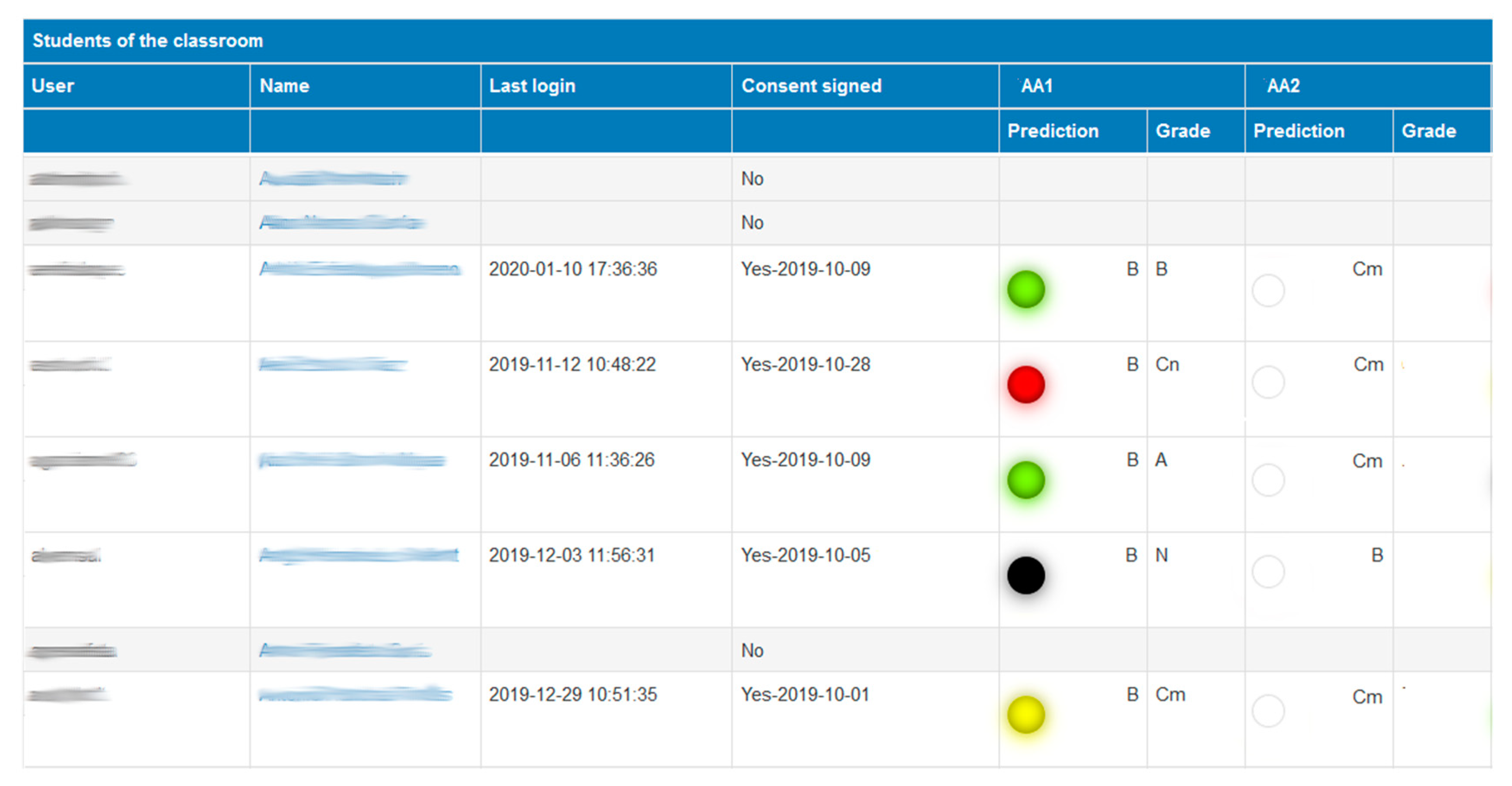


