An Accurate and Efficient Approach to Calculating the Wheel Location and Orientation for CNC Flute-Grinding

Abstract

The profile of flutes has a great influence on the stiffness and chip-removal capacity of end-mills. Generally, the accuracy of flute parameters is determined by the computer numerical control (CNC) grinding machine through setting the wheel’s location and orientation. In this work, a novel algorithm was proposed to optimize the wheel’s location and orientation for the flute-grinding to achieve higher accuracy and efficiency. Based on the geometrical constraint that the grinding wheel should always intersect with the bar-stock while grinding the flutes, the grinding wheel and bar-stock were simplified as an ellipse and circle via projecting in the cross-section. In light of this, we re-formulated the wheel’s determination model and analyzed the geometrical constraints for interference, over-cut and undercut in a unified framework. Then, the projection model and geometrical constraints were integrated with the evolution algorithm (i.e., particle swarm optimization (PSO), genetic algorithm (GA) for the population initialization and local search operator so as to optimize the wheel’s location and orientation. Numerical examples were given to confirm the validity and efficiency of the proposed approach. Compared with the existing approaches, the present approach improves the flute-grinding accuracy and robustness with a wide range of applications for various flute sizes. The proposed algorithm could be used to facilitate the general flute-grinding operations. In the future, this method could be extended to more complex grinding operations with the requirement of high accuracy, such as various-section cutting-edge resharpening.

1. Introduction

Flutes, as the major structure of end-mills, play an important role in the cutting performance [1,2,3,4]. A flute can be defined by the following three parameters: core radius, flute angle and rake angle [5,6,7]. The rake angle influences the cutting force, while the core radius and the helix angle determine the stiffness and chip-removal capacity of the cutters. The performance of those flute parameters quietly depends on the manufacturing accuracy. Generally, the flute is manufactured by the CNC grinding machine through the determination of location and orientation for the grinding wheel path [8,9,10]. In the flute-grinding operations, the grinding wheel will move with a helix path to generate the grooves. In recent years, much attention has been paid to developing an advanced wheel path determination model and optimized algorithms for the CNC flute grinding to minimize the manufacture errors and improve calculation efficiency.

The kinematics of flute-grinding operations for CNC grinders has been developed by many researchers. For instance, Kim et al. [11] developed a simulation method with Boolean operations to construct the helix motion and developed an iterative process to compute the wheel geometry and location data. Although this method could be used for virtual cutting tests in the CAM system, it is time-consuming to achieve a high machining accuracy. To improve the precision of generated flutes, Li [12] established a novel algorithm to calculate the numerical data of flutes based on the enveloping theory, in which the flute profile was interpolated with appropriate discrete points using the cubic polynomial expression. However, this method might be invalid for grinding with a bevel-type wheel. In order to calculate the location and orientation of wheels with complex shapes (e.g., 1B1, 1E1, 1F1, and 4Y1 wheels), Habibi et al. [13] used virtual grinding curves to formulate the grinding processes. Based on the virtual curves, they calculated the grinding error with the worn wheels and compensated the wheel path. Generally, the kinematic of flute-grinding was represented by several transcendental equations, which were supposed to be solved to get the generated helical flute. However, it is very complicated to give the analytical solution, and thus numerical analysis was generally used to describe the flute profile in current studies, which suffer from long computation time. For free-form grinding wheels, Wasif et al. [14] presented a novel method for five-axis CNC grinding through the optimization of the grinding wheel geometry, which was constructed with line segments and circular arcs. Although this method could economically produce or dress the grinding wheel for accurately grinding the end-mill cutters, it ignored the optimization of the wheels’ path. On the basis of the flute-grinding model, the following problem is how to achieve the desired flute parameters by setting the trajectory of the grinding wheel. In industry, the conventional way is to grind end-mill flutes by trial and error, which is costly and time-consuming [15]. Mathematically, the desired flute profile can be viewed as an optimization problem with regards to the wheel’s shape and configuration. To solve this problem, Chen et al. [16] proposed an iteration algorithm to determine the wheel location and orientation. For each loop, the generated flute parameters were compared with the desired values until they converged within the target range. The iteration method has a high calculating speed and precision, but it required a proper initial value, which cannot be easily determined without experience. In Karpuschewski’s research [17], particle swarm optimization (PSO) was investigated to search the wheel location for a given helical flute and grinding wheel profile. Recently, Li et al. [18] extended this work with a novel graphic analysis method and niche particle swarm optimization (NPSO) algorithm to solve the problem for multi-objective of machining accuracy. Although the evolution algorithms (EA, i.e., PSO, GA) could be used in the wheel path optimization process with a global search strategy for such a complex nonlinear problem, they are not stable in convergence, especially for some small flutes (flute diameter < 1 mm).

In view of the above survey, it can be seen that the current study has addressed the modeling of flute-grinding well, but fast and stable algorithms are still required for further study. Currently, extreme-size cutters are widely used in industry, such as the micro-milling cutter or turbine blade root milling cutter. The flute parameters for those cutters will greatly affect their cutting performance, which requires higher accuracy. However, the current algorithms lack the definition of various constraint conditions in machining, which cannot guarantee the machining accuracy and calculation stability. In this work, a new method is presented to calculate the flute parameters and determine its CNC grinding operations. Compared to the above studies, we projected the grinding wheel in the cross-section and used a two-parameter operator to control the grinding operations. Regarding the wheel path optimization algorithm, the projection model was integrated with the evolution algorithm (i.e., PSO, GA) for the population initialization and local search operator. Compared to the current EA method, the improved method showed better stability and short computation time. In addition, it could achieve higher accuracy for a wide range of flute sizes with various profiles, especially for the above-mentioned small flutes.

The outline of the paper is described as follows. In Section 2, the kinematic of flute-grinding is a model with an explicit expression, and the generated flute parameters are formulated. In Section 3, a projection model is proposed for the grinding processes and a two-parameter operator to control the wheel location and orientation is introduced. Additionally, the constraints for undercut, over-cut and extreme-cut of flutes are investigated. This projection model will integrate with the subsequent evolution algorithm. Section 4 presents a wide range of flute-grinding problems to test the accuracy, efficiency, and robustness of the proposed method. Finally, Section 5 summarizes the whole article and points out the contribution of our work.

2. Modeling of Flute-grinding Processes

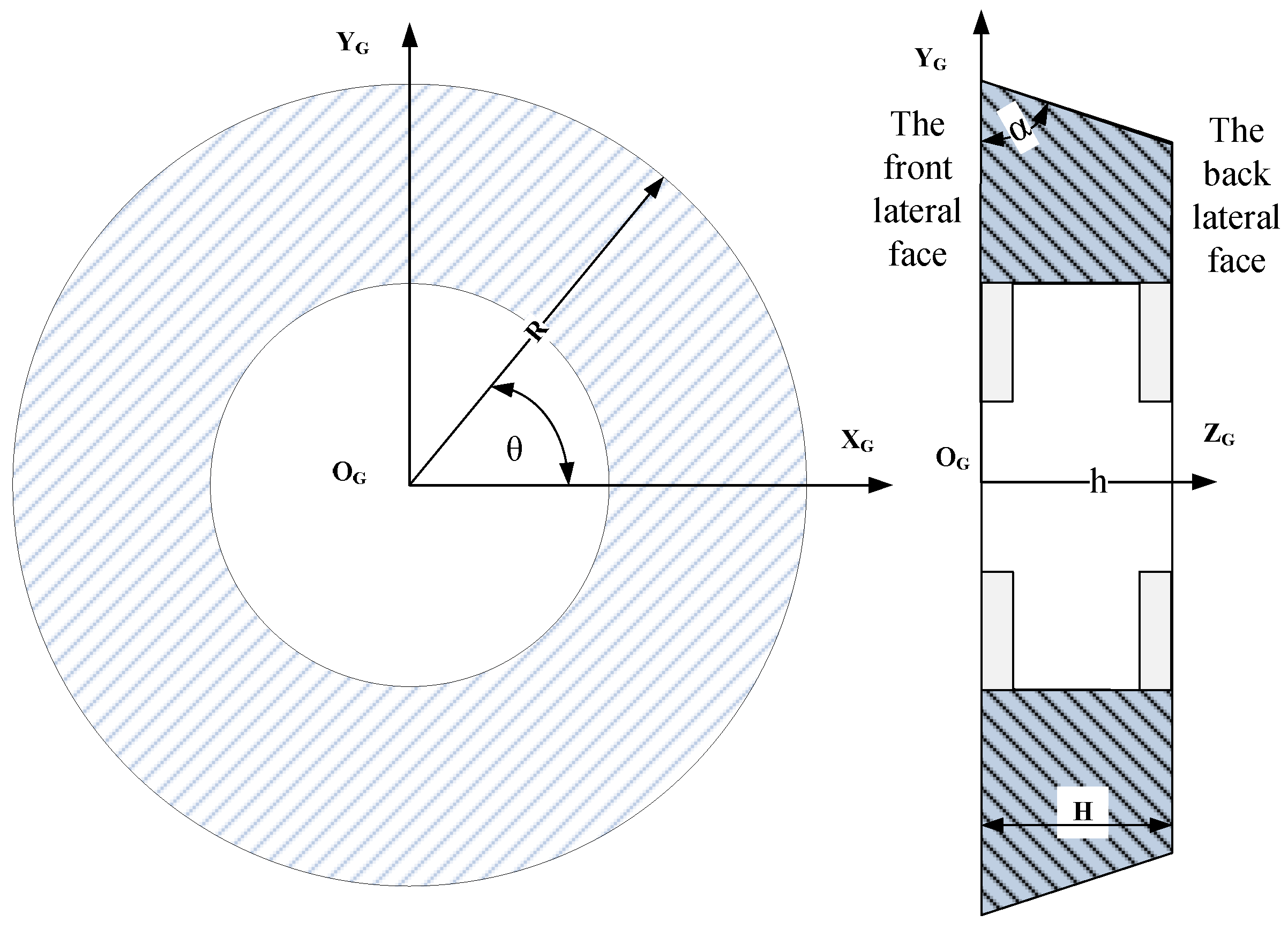
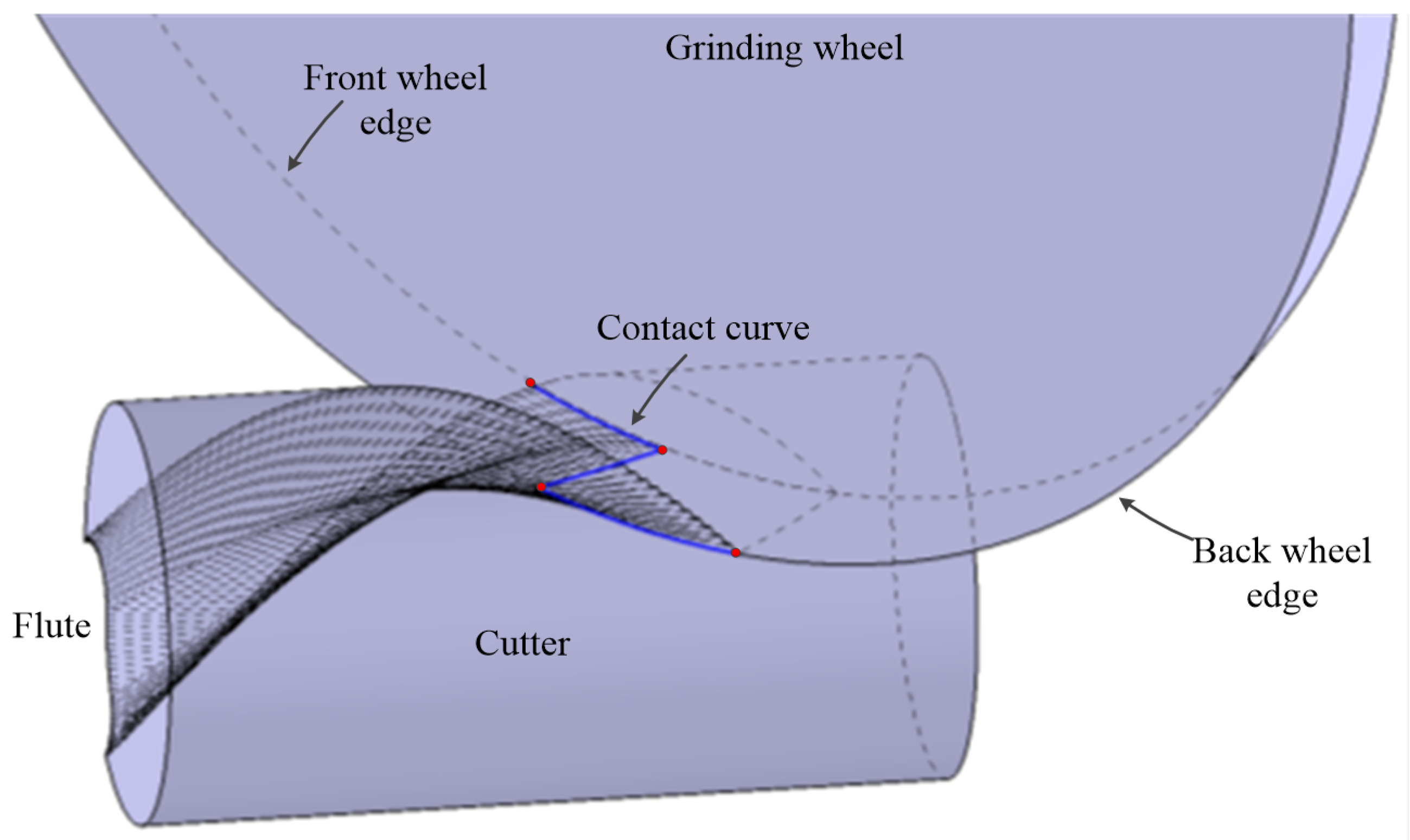
2.1. Grinding Wheel Modeling

In this work, a standard conical grinding wheel was applied to implement the flute-grinding. Figure 1 illustrates this type of standard grinding wheel. To describe the wheel’s geometry, a frame $O_G$, denoted as a wheel coordinate system, is developed and shown in Figure 1. Then, the parametric representation of the wheel ${}^{G}W\left(h,\theta \right)$ in the wheel coordinate system can be derived as

$${}^{G}W\left(h,\theta \right)=\left[\begin{array}{c}f\cdot \cos \theta \\ f\cdot \sin \theta \\ h\end{array}\right],$$

(1)

where $h\in \left[0,\mathrm{H}\right]$, $\theta \in \left[0,2\pi \right]$ and $f=\mathrm{R}-h\cot \alpha$.

Except for the wheel surface, the lateral face will also be involved in the grinding processes. Geometrically, the front lateral face ${}^{G}W\left(0,\theta \right)$ and the back lateral face ${}^{G}W\left(\mathrm{H},\theta \right)$ can be obtained by setting $h=0$ and $h=\mathrm{H}$. Additionally, the wheel surface normal is deduced from Equation (1) as follows:

$${}^{G}N=\left[\begin{array}{c}\cos \theta \\ \sin \theta \\ \cot \alpha \end{array}\right]$$

(2)

2.2. Kinematic of CNC Flute-Grinding

To demonstrate the flute-grinding operations, another framework $O_T$ is established in Figure 2, which is denoted as a tool coordinate system. In the modeling, $O_T$ is static while $O_G$ is moving with the grinding wheel. The flute-grinding operations consist of two steps: (1) wheel set-up and (2) wheel moving with a helix trajectory.

In the wheel set-up operation, the wheel is configured in $O_T$ with a specified location and orientation shown in Figure 2. The wheel location is defined by the wheel center $O_G$, which is denoted by the coordinate value $\left[dxdydz\right]$. The wheel orientation is defined as an angle, which can be viewed as rotating the grinding wheel about the $Y_T$ axis in a counter clockwise direction through the angle $\beta$. To this end, the set-up operation in the tool coordinate system can be expressed using the homogeneous transformation matrix in Equation (3).

$${}^{\mathbf{T}}\mathbf{M}_1=\left[\begin{array}{c}\cos \beta \\ 0\\ -\sin \beta \\ 0\end{array}\begin{array}{c}0\\ 1\\ 0\\ 0\end{array}\begin{array}{c}\sin \beta \\ 0\\ \cos \beta \\ 0\end{array}\begin{array}{c}dx\\ dy\\ dz\\ 1\end{array}\right].$$

(3)

In the wheel helix motion, the wheel moves along the $Z_T$ axis with a translation velocity ν while the cutter rotates about the $Z_T$ axis with a velocity ω. In the tool coordinate system, the kinematics matrix of the helix motion is represented as follows:

$${}^{\mathbf{T}}\mathbf{M}_1=\left[\begin{array}{c}\cos \left(\omega \cdot t\right)\\ \sin \left(\omega \cdot t\right)\\ 0\\ 0\end{array}\begin{array}{c}0\\ 1\\ 0\\ 0\end{array}\begin{array}{c}-\sin \left(\omega \cdot t\right)\\ \cos \left(\omega \cdot t\right)\\ 1\\ 0\end{array}\begin{array}{c}0\\ 0\\ v\cdot t\\ 1\end{array}\right],$$

(4)

where $t$ represents the grinding time.

To guarantee the helix angle $\lambda$, the translation $v$ and the rotation $\omega$ is supposed to satisfy the following condition:

$$\cot \lambda =\frac{v}{r_T\cdot \omega }.$$

(5)

Based on the above operations, the kinematic of grinding wheels can be obtained with regarding machining time t in the tool coordinate system by integrating Equations (1)–(5), listed in Equation (6). In addition, to simplify the calculation, the rotation speed ω is generally set as 1 in the following equations.

$$\begin{array}{l}{}^{T}W\left(h,\theta ,t\right)={}^{T}M_2\cdot {}^{T}M_1\cdot {}^{G}W\left(h,\theta \right)=\\ \left[\begin{array}{c}dx\cdot \cos t-dy\cdot \sin t+h\cdot \sin \beta \cdot \cos t-f\cdot \sin \theta \cdot \sin t+f\cdot \cos \beta \cdot \cos \theta \cdot \cos t\\ dy\cdot \cos t+dx\cdot \sin t+h\cdot \sin \beta \cdot \sin t+f\cdot \sin \theta \cdot \cos t+f\cdot \cos \beta \cdot \cos \theta \cdot \sin t\\ h\cdot \cos \beta +v\cdot t-f\cdot \sin \beta \cdot \cos \theta +dz\end{array}\right]\end{array}.$$

(6)

Geometrically, the flutes are generated by the envelope of grinding wheels. The envelope surface consists of a group of curves, which are called the contact curve [19]. As shown in Figure 3, the contact curve is composed of two parts. One is generated by the wheel surface, which can be deduced using envelope theory. The other is formed by part of the wheel edges.

For the first part of the contact curve, it can be obtained using the conjugate theory as shown in Equation (7):

$${}^{T}N\cdot {}^{T}V=0,$$

(7)

where ${}^{T}N={}^{T}M_2\cdot {}^{T}M_1\cdot {}^{G}N$ and ${}^{T}V\left(h,\theta ,t\right)=\frac{d\left({}^{T}W\left(h,\theta ,t\right)\right)}{dt}$.

By solving Equation (7), the equation of this contact curve can be deduced as Equation (8).

$$v\cdot \left(dz-\sin \beta \cdot \cos \theta +\cot \alpha \cdot \cos \beta \right)-\left(dy+\sin \theta \cdot f\right)\cdot \left(dx+\cot \alpha \cdot \sin \beta +\cos \beta \cdot \cos \theta \right)+\left(dy+\sin \theta \right)\cdot \left(dx+h\cdot \sin \beta +\cos \beta \cdot \cos \theta \cdot f\right)=0.$$

(8)

By solving this triangular equation, the explicit expression of the contact curve can be obtained in Equation (9):

$${\theta }^{*}=a\tan 2\left(B,A\right)+a\tan 2\left(\sqrt{A^2+B^2-C^2},C\right),$$

(9)

where $\{\begin{array}{c}A=-dy\cdot \cos \beta -v\cdot \sin \beta \\ B=dx+f\cdot \sin \beta \cdot \cot \alpha \\ C=dy\cdot \cot \alpha \cdot \sin \beta -dz\cdot v-v\cdot \cot \alpha \cdot \cos \beta \end{array}$.

Substituting Equation (9) into Equation (6), the first part of the flute surface can be obtained, which is formed by the envelope of the wheel surface in a general form in Equation (10).

$${}^{T}W\left(h,t\right)=\left[\begin{array}{c}dx\cdot \cos t-dy\cdot \sin t+h\cdot \sin \beta \cdot \cos t-f\cdot \sin {\theta }^{*}\cdot \sin t+f\cdot \cos \beta \cdot \cos {\theta }^{*}\cdot \cos t\\ dy\cdot \cos t+dx\cdot \sin t+h\cdot \sin \beta \cdot \sin t+f\cdot \sin {\theta }^{*}\cdot \cos t+f\cdot \cos \beta \cdot \cos {\theta }^{*}\cdot \sin t\\ h\cdot \cos \beta +v\cdot t-f\cdot \sin \beta \cdot \cos {\theta }^{*}+dz\end{array}\right]$$

(10)

The other part of the contact curve generated by wheel edge can be obtained by setting $h=0$ or $h=\mathrm{H}$ for Equation (6) denoted as ${}^{T}W\left(0,\theta ,t\right)$ and ${}^{T}W\left(\mathrm{H},\theta ,t\right)$.

Generally, the flute parameters are presented in the cross-section with the definition of core radius, flute angle and rake angle [20,21]. The flute profile could be easily obtained by setting Z = 0 for Equation (10), as shown in Equation (11):

$${}^{T}W\left(h\right)=\left[\begin{array}{c}{x}_c\\ y_c\end{array}\right]= \left[\begin{array}{c}dx\cdot \cos t^{*}-dy\cdot \sin t^{*}+h\cdot \sin \beta \cdot \cos t^{*}-f\cdot \sin \beta \cdot \sin t^{*}+f\cdot \cos \beta \cdot \cos {\theta }^{*}\cdot \cos t^{*}\\ dy\cdot \cos t^{*}+dx\cdot \sin t^{*}+h\cdot \sin \beta \cdot \sin t^{*}+f\cdot \sin \beta \cdot \cos t^{*}+f\cdot \cos \beta \cdot \cos {\theta }^{*}\cdot \sin t^{*}\end{array}\right],$$

(11)

where $t^{*}=\frac{R\cdot \sin \beta \cdot \cos {\theta }^{*}-h\cdot \cos \beta -dz}{v}$.

As shown in Figure 4a, the flute parameters are defined as follows:

The flute angle is established as the opening angle between the vector $O_T{P}_1$ and another vector $O_T{P}_2$, which can be calculated using: $\varphi =\mathrm{acos}\left(O_T{P}_1\cdot O_T{P}_2\right).$

The core radius is the minimum distance from a point $O_T$ to the flute profile, which can be calculated as: $r_c=\min \left(x_c{}^2+y_c{}^2\right)$.

The rake angle is illustrated in Figure 4b, which is a close-up of Figure 4a at point $P_1$. In practice, the rake angle is measured at the start point $P_3$ with a measure distance $PD$ ($PD$ is set as 5% of tool radius in this work). Geometrically, the rake angle is the included angle of the two vectors $P_2{O}_T$ and $P_2{P}_3$, which can be expressed as: $\gamma =\mathrm{acos}\left(P_2{O}_T\cdot P_2{P}_3\right)$

In addition, the points $P_1$, $P_2$ and $P_3$ can be obtained by the following conditions:

(1)

Point $P_1$ is deduced by Equation (10) satisfying the condition $\sqrt{x_c^2+y_c^2}=r_T$;

(2)

Point $P_2$ is deduced by setting $h=0$ to Equation (10), and satisfying the condition $\sqrt{x_c^2+y_c^2}=r_T$;

(3)

Point $P_3$ is deduced by setting $\left|P_2{P}_3\right|=\mathrm{PD}=5\%\cdot r_T$.

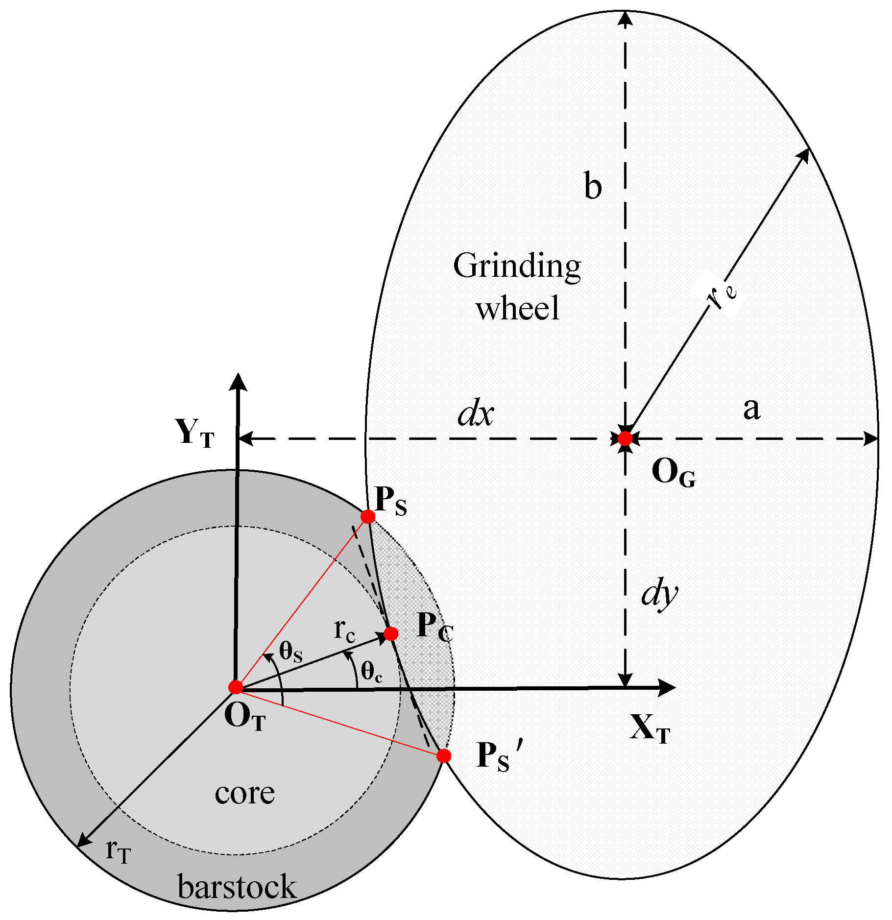
3. Determination of Wheel Location and Orientations with a 2D Projection

Mathematically, the flute-grinding operations can be simplified with three equations shown in Equation (12). For these equations, the wheel location $\left[dxdy\right]$ and orientation $\beta$ are supposed to be calculated to configure the wheel path and generate the designed flute profile. Generally, the intelligent evolution algorithms, i.e., GA or PSO, were used to solve the above equations. However, it was reported that the selection of initial points would greatly affect the accuracy and efficiency of the optimization. In practice, we found that the initial wheel’s location and orientation were confined by several geometrical conditions, such as inference avoidance, contact constraints, etc., which can be used to define the feasible space for the initial points. To this end, an optimization method was introduced to build the feasible space and constraints by mapping the grinding operations into a two-dimensional projection.

$$\{\begin{array}{c}{f}_{ rake} \left(dx,dy,\beta \right)={\gamma }_0\\ f{ }_{flute }\left(dx,dy,\beta \right)={\varphi }_0\\ f{ }_{core} \left(dx,dy,\beta \right)=r_{c0}\end{array}.$$

(12)

3.1. Grinding Operation Projection

Geometrically, the flutes are formed by the intersection between the wheel and the bar-stock. To represent the intersection, the grinding wheel and the bar-stock were projected in the cross-section, which is shown in Figure 5. The bar-stock is simplified as a circle area and the wheel edge can be expressed with an ellipse area. The ellipse could be represented with regard to the wheel’s location and orientation denoted as ${r_e|}_{\left(dx,dy,\beta \right)}$. In order to assure the accuracy of the core radius, the ellipse will intersect with the circle $r_T$ and tangent with the circle $r_c$ at a tangent point. The tangent point is defined by the parameter ${\theta }_c$, denoted by ${{\mathrm{P}}_{\mathrm{c}}|}_{\left({\theta }_c\right)}$. It can be seen that the point ${{\mathrm{P}}_{\mathrm{c}}|}_{\left({\theta }_c\right)}$ can be used to locate the ellipse. The algebra relation between ${{\mathrm{P}}_{\mathrm{c}}|}_{\left({\theta }_c\right)}$ and ${r_e|}_{\left(dx,dy,\beta \right)}$ is deduced in Appendix A. In light of the above geometrical relation, the wheel path determination equation can be re-organized concerning the parameters ${\theta }_c$ and $\beta$, shown in Equation (13).

$$\{\begin{array}{c}{f}_{ rake} \left({\theta }_C, \beta \right)={\gamma }_0\\ f{ }_{flute }\left({\theta }_C, \beta \right)={\varphi }_0\\ f{ }_{core} \left({\theta }_C, \beta \right)=r_{c0}\end{array},$$

(13)

To solve this equation, an optimization model is defined as following:

$$min\xi \left({\theta }_C, \beta \right)=s.t.\xi =max\left\{\left|\frac{f_{ rake}\left({\theta }_C, \beta \right)-{\gamma }_0}{{\gamma }_0}\right|,\left|\frac{f_{flute}\left({\theta }_C, \beta \right)-{\varphi }_0}{{\varphi }_0}\right|,\left|\frac{f_{core}\left({\theta }_C, \beta \right)-r_{c0}}{r_{c0}}\right|\right\},$$

(14)

where $\xi$ is the grinding error in the following description.

In addition, several constraints were defined as follows:

• Constraint 1: the tangent point ${{\mathrm{P}}_{\mathrm{c}}|}_{\left({\theta }_c\right)}$ should always locate in the first or the second quadrant,

  $${\theta }_C\in \left[0,\pi \right].$$

  (15)
• Constraint 2: the wheel edge cannot be separated with the bar-stock and overcut the core radius,

  $$r_c\left({\theta }_C, \beta \right)=\left|{\mathrm{O}}_{\mathrm{T}}{\mathrm{P}}_{\mathrm{C}}\right|\in \left[r_{c0},r_T\right],$$

  (16)
• Constraint 3: to avoid interference, the open-angle ${\theta }_S$ should satisfy the following condition (see Appendix B),

  $${\theta }_S\ge \Omega ,$$

  (17)

To sum up, the flute-grinding operations can be re-formulated by the following optimization problem:

$$\min \xi \left({\theta }_C, \beta \right),$$

subjected to: Equations (15)–(17).

Compared with current flute-grinding optimization models, this project method has two advantages: (1) instead of three decision parameters $\left(dx,dy,\beta \right)$, only two parameters $\left({\theta }_C,\beta \right)$ were required to be considered, which will simplify the calculation during the iterations; (2) three constraints could be used to confine the feasible area and generate the proper initial points, which would improve the robustness and efficiency of the optimization.

3.2. Calculation Procedure with the Improved GA and PSO

To solve the above-constrained optimization problem, the projection model with the GA and PSO was integrated to calculate the wheel’s location and orientation for flute-grinding operation. As mentioned, the initial points would greatly affect the optimization results. In this work, an initial points generation algorithm was proposed in Algorithm 1, which could be used for the population initialization for GA or PSO. It is noted that all the initial points would be checked by the over-cut and interference constraints in the projection model. Furthermore, the flowchart of improved GA and PSO (IGA, IPSO) integrated with the projection model is shown in Figure 6. First, a set of initial points were generated with the algorithm in, which is used to calculate the following wheel’s location and the generated flute parameters. In light of this, the grinding errors were evaluated and set as the fitness function for the GA and PSO. For the IGA and IPSO, the off springs or particles generated by the iteration operators, e.g., mutation or crossover, will be checked by the proposed over-cut and interference constraints. The iteration will stop while satisfying either of the following conditions: (1) iterations n > 100 (2) there is no obvious improvement in the grinding errors within n = 10 succeeding iterations. With this procedure, the optimized wheel’s location and orientation, the generated flute parameters and grinding errors could be obtained.

Algorithm 1 Generate N initial points

Input: Desired flute $\left\{r_T,\lambda ,r_{c0},{\gamma }_0,{\varphi }_0\right\}$ and wheel parameters $\left\{R,H,\alpha \right\}$

Output: initial points (pop) for $\beta$ & ${\theta }_C$

1.  $pop=\left\{\phi \right\}$.

2. while n < N do

3.      $\beta =\mathrm{random}\left(0,\pi /2\right)$ and ${\theta }_C=\mathrm{random}\left(0,\pi \right)$.

4.       Calculate $r_c\left({\theta }_C,\beta \right)$ and ${\theta }_s$ in the projection model (see Appendix A)

5.      If satisfy the constraints for Equation (16) and Equation (17).

6.      $pop=pop{\displaystyle \cup }\left\{\beta ,{\theta }_C\right\}$

7.      else

8.       go to line 3

9.     end if

10. return pop

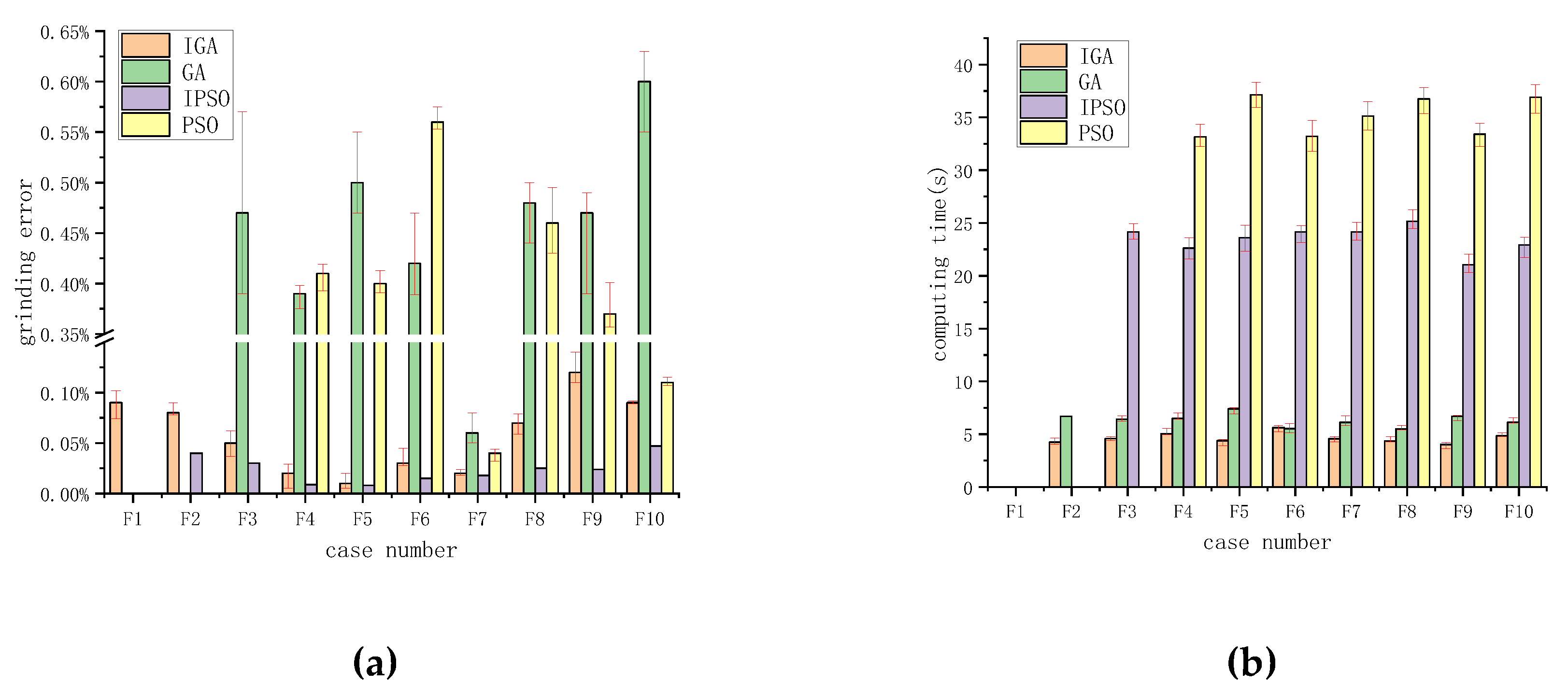
4. Numerical Simulation

To test the accuracy and efficiency of the presented model, the numerical simulation was conducted with various sizes of flutes. Three types of grinding wheels were provided in

Table 1. Specification of grinding wheel.

Wheel Parameters	Wheel 1	Wheel 2	Wheel 3
wheel width H (mm)	5	20	40
wheel radius R (mm)	30	75	75
wheel angle α (deg.)	75	75	90

. The designed flutes were divided into three groups according to their size: small ($r_T\le 1\mathrm{mm}$), medium ($1\mathrm{mm}\le r_T\le 20\mathrm{mm}$), large ($r_T\ge 20\mathrm{mm}$). To grind those flutes, the wheel’s location and orientation in CNC operations were determined with the proposed improved GA and PSO (IGA, IPSO), and also compared with the traditional GA and PSO. For each instance, the optimization was run 10 times and the average results and deviation were recorded. The optimization program was implemented in MATLAB 2010 on a computer with Intel Core i5, 2.39 GHz, 4 GB RAM. The parameters of the GA and PSO were set in

Table 2. Parameters of optimization algorithms.

Algorithm	Parameters Setting
GA or IGA	initial population size: 100 range of crossover probability: 0.2 range of mutation probability: 0.1 stopping condition: iterations > 100 or $\xi$ < 1 × 10−4
PSO or IPSO	initial population size: 100 inertia weight: 1 inertia weight damping Ratio: 0.99 personal learning coefficient: 1.5 global learning coefficient: 2.0 stopping condition: iterations >1 00 or $\xi$ < 1 × 10−4

. The desired flutes parameters are listed in

Table 3. The machined flute parameters.

Flute Size	Case No.	Cutter Radius	Desired Flute Parameters 1	Flute Parameters Solved by IGA	Flute Parameters Solved by GA	Flute Parameters Solved by IPSO	Flute Parameters Solved by PSO
small size flutes	F1	0.3	(0.2, 6, 75)	(0.200, 5.995, 74.956)	/	/	/
	F2	0.5	(0.3, 6, 75)	(0.300, 5.996, 74.976)	/	(0.300, 5.919, 74.796)	/
	F3	1	(0.6, 6, 75)	(0.600, 5.998, 75.962)	(0.602, 5.991, 75.386)	(0.600, 6.000, 75.027)	/
medium size flutes	F4	7	(5, 9, 75)	(5.000, 9.005, 75.016)	(4.989, 8.963, 75.007)	(5.000, 9.000, 74.997)	(5.021, 8.985, 74.781)
	F5	9	(5, 9, 75)	(5.000, 8.996,75.009)	(5.149, 8.894, 75.410)	(5.000, 9.000,75.000)	(4.973, 8.969, 74.926)
	F6	11	(6, 25, 110)	(6.000, 25.016, 109.981)	(5.955, 25.037, 109.530)	(6.000, 25.000,110.002)	(5.946, 24.994, 109.591)
	F7	17	(10, 9, 75)	(10.000, 9.002, 75.005)	(9.997, 9.006, 74.916)	(10.000, 8.998,75.003)	(9.995, 8.984,74.989)
large size flutes	F8	20	(15, 9, 75)	(15.000, 8.995, 75.942)	(14.934, 9.038, 75.343)	(15.000, 9.000, 75.003)	(14.979, 8.995, 75.139)
	F9	25	(17, 25, 110)	(17.000, 24.995, 110.143)	(17.081, 25.071, 109.598)	(17.000, 25.000, 109.998)	(16.929, 24.919, 110.406)
	F10	30	(20, 9, 75)	(20.000, 9.008, 75.047)	(20.129, 9.020, 75.399)	(20.000, 9.000, 74.999)	(20.018, 9.011, 75.109

¹ Note: (core radius, rake angle and flute angle).

. The helix angle for those flutes was set as 30 degrees.

The simulation results with various algorithms are given in Table 3. It can be concluded that the integrated method, i.e., IGA and IPSO, had wider applicability and higher accuracy than the traditional GA and PSO. Especially for IGA, it could be used to solve the very small size flute-grinding problem. For further study, the grinding errors $\xi$ (calculated by Equation (14)) between the grinding flute parameters and the designed flute parameters were calculated as shown in Figure 7a. It can be seen that the integrated method superior to the traditional in accuracy and stability. The accuracy of flute parameters with IGA and IPSO could achieve 1 × 10⁻⁴. It was also noted that the grinding errors with IGA and IPSO were less for the medium size flutes, while larger for the small and large size flutes. What is more, to further test the efficiency of the proposed method, the computing time was recorded as shown in Figure 7b. The integrated method also showed better efficiency in convergence, which could save about 15%–40% computing time. In addition, the initial setting parameters of the grinding wheel solved by IGA are provided in

Table 4. Initial setting parameters of grinding wheels calculated by IGA.

Case No.	β	θc	dx	dy
F1	52.9353	87.7783	0.4304	30.1917
F2	50.3040	82.2274	1.7030	30.1838
F3	49.6645	82.7015	1.6804	30.4926
F4	53.2624	95.5550	−3.0894	80.4462
F5	48.4607	80.5059	6.3067	79.4745
F6	55.3177	100.8935	−5.7797	80.4662
F7	48.4607	77.1924	9.5815	83.9187
F8	54.5717	85.3600	3.2566	89.8680
F9	57.7373	99.4303	−6.3210	91.4772
F10	52.8445	79.5509	8.6418	94.2074

. In light of the IGA solution, three instances were selected and simulated in the software CATIA. The simulated results were obtained and measured, as shown in Figure 8, which also shows that they are highly consistent with the designed flute parameters. In summary, according to the simulation tests for various optimization methods, it is demonstrated that the proposed IGA and IPSO based on the projection model is effective, efficient, and robust solving the flute-grinding problem.

5. Conclusions

In the CNC flute-grinding processes, the accuracy of generated flute parameters is determined by setting the wheel’s location and orientation. The existing methods for the solution of wheel path optimization were time-consuming and cannot handle grinding the extreme-size cutters. In addition, the current model ignored the definition of various constraints in machining, which would strongly affect the machining accuracy and calculation stability.

In the present work, a novel projection model for flute-grinding operations was developed to generate the grinding wheels’ configuration. Based on the projection model, the wheel’s location was re-formulated with the projection parameters, which simplified the following calculation of machined flute parameters. To minimize the flute-grinding errors regarding the wheel configuration, the projection model was used to generate the proper initial points and was integrated with the GA and PSO as a heuristic regulation. In the numerical simulation, the improved GA and PSO are more accurate, efficient, and robust, with a wide range of applications for various flute sizes. It is noted that the proposed flute-grinding algorithm was verified with a simulation-based method. For the actual grinding, a great deal of topics, such as the dynamics of the grinding machine, the material of the grinding wheel and work-piece, the post-processing, the grinding speed, etc., should be considered in the future experiments.

References

1. Jiang, F.; Zhang, T.; Yan, L. Analytical model of milling forces based on time-variant sculptured shear surface. Int. J. Mech. Sci. 2016, 115–116, 190–201. [Google Scholar] [CrossRef]
2. Yan, L.; Rong, Y.M.; Jiang, F.; Zhou, Z.X. Three-dimension surface characterization of grinding wheel using white light interferometer. Int. J. Adv. Manuf. Tech. 2011, 55, 133–141. [Google Scholar] [CrossRef]
3. Pimenov, D.; Hassui, A.; Wojciechowski, S.; Mia, M.; Magri, A.; Suyama, D.; Bustillo, A.; Krolczyk, G.; Gupta, M. Effect of the Relative Position of the Face Milling Tool towards the Workpiece on Machined Surface Roughness and Milling Dynamics. Appl. Sci. 2019, 9, 842. [Google Scholar] [CrossRef] [Green Version]
4. Mei, Y.; Mo, R.; Sun, H.; He, B.; Bu, K. Stability Analysis of Milling Process with Multiple Delays. Appl. Sci. 2020, 10, 3646. [Google Scholar] [CrossRef]
5. Ren, L.; Wang, S.; Yi, L.; Sun, S. An accurate method for five-axis flute grinding in cylindrical end-mills using standard 1V1/1A1 grinding wheels. Precis. Eng. 2016, 43, 387–394. [Google Scholar] [CrossRef]
6. Xiao, S.; Wang, L.; Chen, Z.C.; Wang, S.; Tan, A. A New and Accurate Mathematical Model for Computer Numerically Controlled Programming of 4Y1 Wheels in 21/2-Axis Flute Grinding of Cylindrical End-Mills. J. Manuf. Sci. Eng. 2013, 135, 04100801–04100811. [Google Scholar] [CrossRef]
7. Pham, T.T.; Ko, S.L. A manufacturing model of an end mill using a five-axis CNC grinding machine. Int. J. Adv. Manuf. Tech. 2010, 48, 461–472. [Google Scholar] [CrossRef]
8. Li, G.; Sun, J.; Li, J. Process modeling of end mill groove machining based on Boolean method. Int. J. Adv. Manuf. Tech. 2014, 75, 959–966. [Google Scholar] [CrossRef]
9. Liu, G.; Wei, W.; Dong, X.; Rui, C.; Liu, P.; Li, H. Relief grinding of planar double-enveloping worm gear hob using a four-axis CNC grinding machine. Int. J. Adv. Manuf. Tech. 2017, 89, 3631–3640. [Google Scholar] [CrossRef]
10. Van-Hien, N.; Ko, S. A New Method for Determination of Wheel Location in Machining Helical Flute of End Mill. J. Manuf. Sci. Eng. 2016, 138, 11100301–11100311. [Google Scholar]
11. Kim, J.H.; Park, J.W.; Ko, T.J. End mill design and machining via cutting simulation. Comput. Aided Design 2008, 40, 324–333. [Google Scholar] [CrossRef]
12. Li, G. A new algorithm to solve the grinding wheel profile for end mill groove machining. Int. J. Adv. Manuf. Tech. 2017, 90, 775–784. [Google Scholar] [CrossRef]
13. Habibi, M.; Chen, Z.C. A Generic and Efficient Approach to Determining Locations and Orientations of Complex Standard and Worn Wheels for Cutter Flute Grinding Using Characteristics of Virtual Grinding Curves. J. Manuf. Sci. Eng. 2017, 139, 04101801–04101811. [Google Scholar] [CrossRef]
14. Wasif, M.; Iqbal, S.A.; Ahmed, A.; Tufail, M.; Rababah, M. Optimization of simplified grinding wheel geometry for the accurate generation of end-mill cutters using the five-axis CNC grinding process. Int. J. Adv. Manuf. Technol. 2019, 105, 4325–4344. [Google Scholar] [CrossRef]
15. Kang, S.K.; Ehmann, K.F.; Lin, C. A CAD approach to helical groove machining .1. Mathematical model and model solution. Int. J. Mach. Tool. Manuf. 1996, 36, 141–153. [Google Scholar] [CrossRef]
16. Chen, Z.; Ji, W.; He, G.; Liu, X.; Wang, L.; Rong, Y. Iteration based calculation of position and orientation of grinding wheel for solid cutting tool flute grinding. J. Manuf. Process 2018, 36, 209–215. [Google Scholar] [CrossRef]
17. Karpuschewski, B.; Jandecka, K.; Mourek, D. Automatic search for wheel position in flute grinding of cutting tools. Cirp Ann. Manuf. Tech. 2011, 60, 347–350. [Google Scholar] [CrossRef]
18. Li, G.; Zhou, H.; Jing, X.; Tian, G.; Li, L. An intelligent wheel position searching algorithm for cutting tool grooves with diverse machining precision requirements. Int. J. Mach. Tool. Manuf. 2017, 122, 149–160. [Google Scholar] [CrossRef]
19. Li, G.; Zhou, H.; Jing, X.; Tian, G.; Li, L. Modeling of integral cutting tool grooves using envelope theory and numerical methods. Int. J. Adv. Manuf. Tech. 2018, 98, 579–591. [Google Scholar] [CrossRef]
20. Wang, L.; Kong, L.; Li, J.; Chen, Z. A parametric and accurate CAD model of flat end mills based on its grinding operations. Int. J. Precis. Eng. Manuf. 2017, 18, 1363–1370. [Google Scholar] [CrossRef]
21. Wang, L.; Chen, Z.C.; Li, J.; Sun, J. A novel approach to determination of wheel position and orientation for five-axis CNC flute grinding of end mills. Int. J. Adv. Manuf. Tech. 2016, 84, 2499–2514. [Google Scholar] [CrossRef]
Figure 1. Modeling of conical grinding wheel.
Applsci 10 04223 g001
Figure 2. Flute-grinding processes: (a) X T Y T view; (b) X G Y G view.
Applsci 10 04223 g002
Figure 3. Illustration of the flute generation and the contact curve.
Applsci 10 04223 g003
Figure 4. The flute parameters: (a) flute angle and core radius; (b) rake angle.
Applsci 10 04223 g004
Figure 5. Illustration of the projection of the wheel edge and cutter profile within the cross-section.
Applsci 10 04223 g005
Figure 6. Flow chart of the improved genetic algorithm (IGA) and improved particle swarm optimization (IPSO) with the projection model.
Applsci 10 04223 g006
Figure 7. Comparisons with various algorithms: (a) the grinding errors; (b) the computing time.
Applsci 10 04223 g007
Figure 8. Simulated cutting tool flutes by CATIA.
Applsci 10 04223 g008