Article

Long-Term Characteristics of Prestressing Force in Post-Tensioned Structures Measured Using Smart Strands

1
Department of Infrastructure Safety Research, Korea Institute of Civil Engineering and Building Technology, 283, Goyang-daero, Ilsanseo-gu, Goyang-si, Gyeonggi-do 10223, Korea
2
Department of Civil Systems Engineering, Ajou University, 206, Worldcup-ro, Yeongtong-gu, Suwon-si, Gyeonggi-do 16499, Korea
*
Author to whom correspondence should be addressed.
Appl. Sci. 2020, 10(12), 4084; https://doi.org/10.3390/app10124084
Submission received: 10 May 2020 / Revised: 30 May 2020 / Accepted: 10 June 2020 / Published: 13 June 2020
(This article belongs to the Section Civil Engineering)

Abstract

:
The proper distribution of prestressing force (PF) is the basis for the design of prestressed concrete (PSC) structures. However, the PF distribution obtained by predictive equations of prestress losses has not been sufficiently validated by comparison with measured data due to the poor reliability and durability of conventional sensing technologies. Therefore, the Smart Strand with embedded fiber optic sensors was developed and applied to PSC structures to investigate the long-term characteristics of PF distribution as affected by concrete creep and shrinkage. The data measured in a 20 m-long full-scale specimen and a 60 m-long PSC girder bridge were analyzed by comparing them with the theoretical estimation obtained from several design equations. Although the long-term decreasing trend of the PF distribution was similar in the measurement and theory, the equation of Eurocode 2 for estimating the long-term prestress losses showed better agreement with the measurement than ACI 209R and ACI 423.10R did. This can be attributed to the more refined form of the predictive equation of Eurocode 2 in dealing with the time-dependency of the PF. The study results also confirmed the need to compensate for the temperature variation in the long-term monitoring to derive the actual mechanical strain related to the PF. We expect our developed Smart Strand to be applied practically in PF measurement for the reasonable safety assessment and maintenance of PSC structures by improving several of the existing drawbacks of conventional sensors.

1. Introduction

Prestressing tendons, such as seven-wire strands in prestressed concrete (PSC) structures, are used to introduce compressive stress in concrete to overcome its low tensile strength against the tensile stresses imposed in service. Therefore, determining the proper distribution of the prestressing force (PF) in the tendons is crucial in the design of PSC structures because it largely affects safety and serviceability. Underestimated or overestimated PF may cause the concrete stresses to vary from those calculated in design, leading to the cracking or crushing of concrete and unexpected camber or deflection. Moreover, PF monitoring is increasingly important to prevent the deterioration or even collapse of PSC structures due to the corrosion or breakage of tendons, as has occurred [1].
The PF varies along the length of a tendon and over time due to the short- and long-term losses of prestress. Although the PF distribution is usually estimated using several predictive equations for the prestress losses during the design of a PSC structure, these equations can only approximate the PF distribution. Although many attempts have been made to validate the theoretical distribution of the PF by using conventional sensing technologies, such as electrical resistance strain gauges (ERSGs), their outcomes were not very successful due to several drawbacks of the ERSGs that led to unreliable data. For example, ERSGs attached to a surface of a strand and lead wires for data acquisition are susceptible to damage during the insertion of strands into a duct, tensioning, and grouting in post-tensioned members [2,3], and at transfer and during the casting of concrete in pre-tensioned members [4,5]. In particular, ERSGs exhibited poor performance for long-term measurement due to inherent low durability when compared to fiber optic sensors [6]. The lifetime of ERSGs is typically much shorter than that of infrastructures.
Therefore, alternative experimental methods, instead of measuring the strains of a strand using ERSGs, have also been adopted to indirectly predict the long-term prestress losses, although the accuracy is decreased. Pessiki et al. [7] employed the crack opening method to estimate the losses in full-scale PSC beams removed from an actual bridge. Garber et al. [8] used vibrating wire gauges to measure the prestress loss in full-scale girder specimens. However, their calculated loss may have been less accurate because the strand strains were derived from the concrete strains obtained from the vibrating wire gauges embedded in concrete at mid-span. The study only provided limited information on the prestress loss at the mid-span. Abdel-Jaber and Glisic [9] monitored long-term prestress loss in a pedestrian bridge using fiber Bragg gratings (FBGs) embedded in a concrete section. As in the case of Garber et al. [8], the strand strains were indirectly derived from these concrete strains. Shing and Kottari [10] compared several predictive equations and field data in terms of the long-term prestress losses in some PSC box girder bridges. However, the field data were not modified by temperature correction, even though the data fluctuated temporally. Furthermore, although the detailed methodology to obtain the field data was not stated, the data showed an unstable trend. Lundqvist and Nilsson [11] also compared the theoretical prestress losses obtained by several predictive equations with the measured losses. However, the comparison was made only at the anchorage of unbonded tendons because of the absence of any data measured inside the tendons using any sensors. In summary, prestress losses were estimated indirectly or measured only at a specific point on a tendon in most of the previous studies due to the limitations of conventional sensing technologies. The complete measurement of the PF distribution along a tendon has very rarely been reported for full-scale specimens or actual infrastructures.
In order to overcome the abovementioned drawbacks and limitations of existing sensing technologies in the estimation of the PF distribution, Smart Strands with embedded fiber optic sensors have been developed recently [2,3]. The Smart Strands were applied to a 20 m-long full-scale specimen and a 60 m-long PSC girder bridge to investigate the long-term characteristics of the PF distribution affected by long-term prestress losses. The measured data were compared with the theoretical values obtained by the predictive equations for long-term prestress losses that are specified in several design provisions.

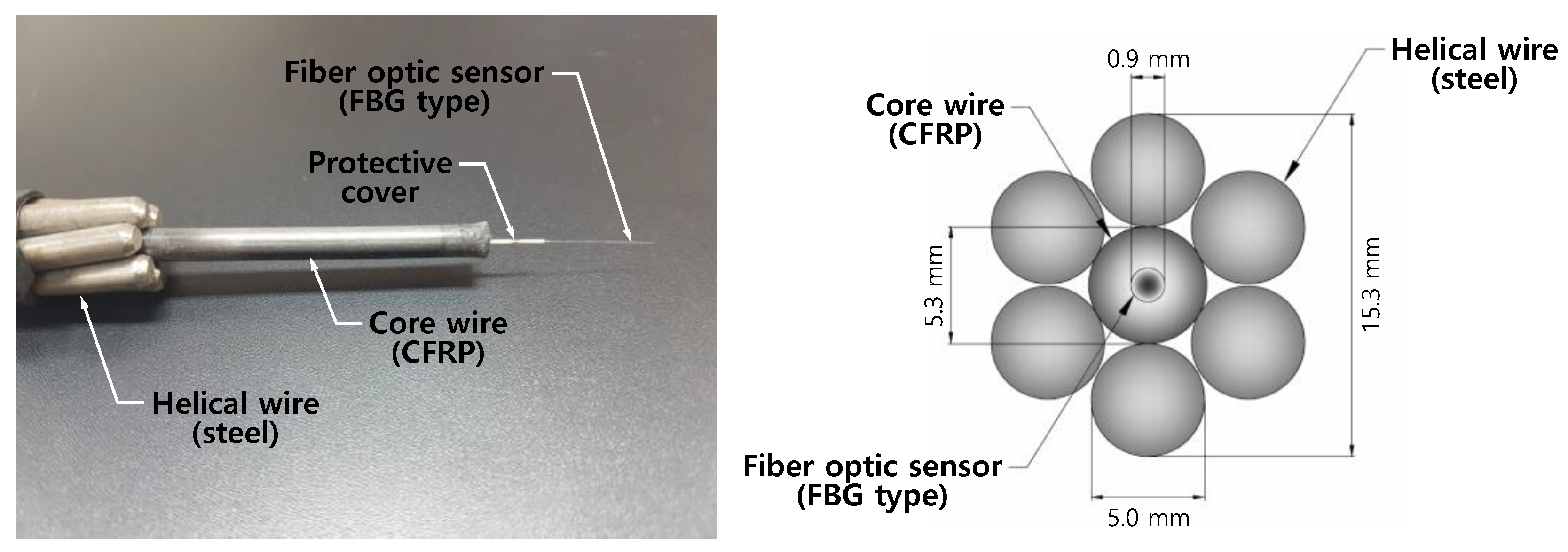
2. Smart Strand with Fiber Optic Sensor

The dimensions of the Smart Strand are almost identical to those of a regular seven-wire strand [12] widely used in PSC structures, as shown in Figure 1. The steel core wire of the regular strand is replaced with carbon fiber reinforced polymer (CFRP) and a fiber optic sensor with several embedded FBGs, while the CFRP core wire is manufactured. The Smart Strand can also play the role of a structural component as a strand because the mechanical properties of the Smart Strand are similar to those of a regular strand in service. The Smart Strand has the following advantages in the measurement of PF when compared to a conventional technique where ERSGs are attached to helical wires of a strand: highly accurate and stable measurement, durability due to the protection provided by embedment, and the measurement of the actual axial strain of a strand. The reliability of the data obtained by Smart Strands was validated by the comparison with those of ERSGs in laboratory tests and a full-scale specimen [2]. If the scope is extended to relatively advanced techniques to measure the PF, other than ERSGs and those introduced in Section 1, the following attempts have been made: vibration and modal analysis [13], ultrasonic waves [14,15], acoustic emission and stress waves [16,17], elasto-magnetic (EM) sensors [18,19], vibrating strings [20], and FBGs encapsulated inside a strand or attached to the surface of a strand [21,22,23,24,25,26,27]. However, many of these methods suffer similar drawbacks to those mentioned earlier in Section 1: they were mainly applied only to laboratory test specimens and were not sufficiently validated through the field measurement of actual full-scale structures. Furthermore, they can only provide approximate and limited data of PF at a specific location. It is noted that a similar type of strand with the FBG-embedded steel core wire was developed in other studies [21,22] and efforts were made to apply this strand to actual structures. Although Shen et al. [27] criticized a type of Smart Strand [2,3,21,22] by mentioning the difficulty in positioning the FBGs at predetermined points and in connecting the fiber optic sensor to an optical cable for data logging, these aspects did not matter, at least in the Smart Strand developed in this study [2,3], according to the authors’ experience. That is, the position of the FBGs on fiber optic sensors can be easily traced by a proper marking technique when the CFRP core wire is manufactured through a pultrusion process and helical wires are assembled around the core wire. Besides, the connection of the fiber optic sensor to the optical cable does not involve much difficulty if the core wire is extruded in advance, as shown in Figure 1.
The wavelength of a reflected light wave measured at each FBG can be converted to the strain at the FBG by Equation (1) when the effect of temperature can be ignored, such as in short-term measurements. However, the temperature should be compensated, as shown in Equation (2), to separate the temperature effect from the total strain. The resulting actual mechanical strain is obtained from long-term measurements over a wide range of ambient temperatures [28,29,30].
ε = 1 1 p e · Δ λ λ B ,
ε = 1 1 p e [ Δ λ λ B ( α + ξ ) Δ T ] ,
where ε : strain, Pe: photo-elastic coefficient, Δ λ = λ λ B : wavelength shift, λ : measured wavelength, λ B : base wavelength at the start of measurement, α : thermal expansion coefficient, ξ : thermo-optic coefficient, Δ T = T T B : temperature change, T : measured temperature, and T B : base temperature at the start of measurement. For the general optical fiber made of silicon dioxide that was used in this study, p e is 0.22 and ξ ranges from 6 × 10⁻⁶~11 × 10−6/°C, where ξ = 6.2 × 10⁻⁶/°C, as given by the manufacturer, and was used herein. Because the stiffness of the hosting concrete where the Smart Strand was embedded was larger than that of the sensor, the thermal behavior of the sensor was dominated by that of the hosting concrete. Therefore, α of concrete was used, which is 10 × 10−6/°C in general.
The strain obtained in Equations (1) or (2) can further be converted to the PF using the force–strain relationship obtained by experiment and analysis, as shown in Equation (3) [31].
P = ( E p A p ) s m a r t ε p [ A + 1 A { 1 + ( B ε p ) C } ( 1 / C ) ] ,
where P : PF at an FBG, ( E p A p ) s m a r t : equivalent E p A p with the value of 26,600 kN for the Smart Strand, which is the hybrid material of steel and CFRP, E p : modulus of elasticity of a strand, A p : cross-sectional area of a strand, ε p : strain measured at an FBG of a Smart Strand, A : 0.18, B : 104, and C : 9.9. However, the curve plotted by Equation (3) is almost linear over a practical service range of ε p , which can be approximated by Equation (4).
P = ( E p A p ) s m a r t ε p .

3. Long-Term Losses of Prestress

The prestress losses in prestressing tendons can largely be divided into short-term losses (also called instantaneous losses or immediate losses) and long-term losses (also called time-dependent losses). Figure 2 shows the types of the prestress losses and the corresponding PF. Details on each prestress loss can be found in the literature [32]. Although the short-term losses are beyond the scope of this study, the friction coefficients related to friction loss were derived in an innovative way using the Smart Strand in two previous studies [2,3]. The present study focuses on the long-term losses.
The creep loss occurs because a concrete member subjected to compression by prestressing tendons is shortened for a long time due to the creep. Then, the prestressing tendon is also shortened with the prestress loss. The creep loss can be calculated by Equation (5) based on the composite action between concrete and a tendon, as proposed by Zia et al. [33] and adopted in ACI 423.10R [34].
Δ f p C R = n C t f c ,
where Δ f p C R : creep loss, n : modular ratio (= E p / E c ), E p : modulus of elasticity of a strand (200,000 MPa), E c : modulus of elasticity of concrete, which was calculated as a function of specified concrete compressive strength ( f c ) according to ACI 318 [35] in this study, C t : creep coefficient, and f c : compressive stress of concrete at the location of a strand caused by prestressing, self-weight, and superimposed permanent dead loads, where f c can be calculated by Equation (6). Note that 0.9 P i was used instead of P i to approximately account in advance for the reduction of P i during long-term losses [32].
f c = ( 0.9 P i A c + 0.9 P i e p I c e s m ) M d I c e s m ,
where P i : total initial PF (refer to Figure 2), A c : area of the concrete section, I c : second moment of area of the concrete section, e p : eccentricity of the tendon centroid with respect to the concrete centroid, e s m : eccentricity of a specific strand (Smart Strand in this study) of which the stress needs to be obtained, and M d : bending moment due to self-weight and superimposed permanent dead loads. Additionally, e s m was used in Equation (6) instead of e p because the theoretical prestress loss at a Smart Strand, not the average prestress loss of all tendons, needs to be compared with the value measured at the Smart Strand for a reasonable comparison. Concrete creep depends on time, concrete compressive strength, member shape, relative humidity, loading age, type of cement, curing condition, temperature, and concrete stress. Equation (7) in ACI 209R [36], originally proposed by Branson and Kripanarayanan [37], has been frequently used to formulate the time-dependency of creep.
C t = t 0.6 10 + t 0.6 C u ,
where t : time after prestressing (days) and C u : ultimate creep coefficient. Equation (7) was suggested, with C u = 2.35 , for a prestressing age of 7 days for moist-cured concrete and of 1~3 days for steam-cured concrete. Several correction factors are applied to account for other conditions and various effects on the creep [36]. The value of C u varies depending on the provisions; for example, ACI 423.10R [34] suggested 1.6 for post-tensioned members. The final creep loss can be obtained by using C u instead of C t in Equation (5).
The shrinkage of concrete due to drying shrinkage and autogenous shrinkage can also cause prestress loss by the reduction of the length of the prestressing tendon. The shrinkage loss can be expressed by Equation (8).
Δ f p S H = E p ( ε s h ) t ,
where Δ f p S H : shrinkage loss, E p : modulus of elasticity of the strand, and ( ε s h ) t : shrinkage strain. The shrinkage of concrete is affected by such factors as time, concrete compressive strength, member shape, relative humidity, type of cement, and temperature. Equation (9) was proposed by ACI 209R [36] to incorporate the time-dependency of ( ε s h ) t for the moist-curing condition.
( ε s h ) t = t 35 + t ( ε s h ) u ,
where t : time after 7 days of moist curing (days) and ( ε s h ) u : ultimate shrinkage strain with the recommended value of 780 × 10−6 m/m. Various correction factors are applied to reflect other effects on the shrinkage [36]. In comparison, ACI 423.10R [34] suggested ( ε s h ) u by incorporating a few correction factors in Equation (10). The final shrinkage loss can be obtained by using ( ε s h ) u instead of ( ε s h ) t in Equation (8). The shrinkage that occurs after the end of initial wet curing and before tensioning is not considered in the calculation of prestress loss.
( ε s h ) u = 8.2 × 10 6 K s h ( 1 0.0024 V / S ) ( 100 R H ) ,
where K s h : correction factor considering the time between the end of initial wet curing and tensioning, V / S : volume to surface ratio (mm), and R H : relative humidity (%).
On the other hand, whereas the relaxation loss can be estimated using various predictive equations [33,34], it cannot be measured by using strain-based sensors, such as Smart Strand, because the relaxation indicates the reduction in tendon stress under constant strain.
The long-term losses can also be obtained in a combined manner using Equation (11), specified in Eurocode 2 [38]. The notations used in the original Expression (5.46) of Eurocode 2 [38] were partly modified in Equation (11) to be concise and consistent.
Δ f p , C R + S H + R = E p ( ε s h ) t + 0.8 Δ f p R + n C t f c 1 + n A p A c ( 1 + A c I c e p 2 ) ( 1 + 0.8 C t ) ,
where Δ f p R : relaxation loss, all other notations were defined earlier. The original form of e p 2 in Equation (11) can be revised to e p e s m in order to further enhance the accuracy, as explained above for Equation (6). However, f c in Equation (11) should be calculated based on P i instead of 0.9 P i because the long-term variation of P i is already accounted for in the derivation of Equation (11) and is incorporated in the denominator of this equation. The detailed calculation methods of ( ε s h ) t and C t in Equation (11) are different from those of the aforementioned ACI 209R. The Korean design code for highway bridges [39] also uses this form of Equation (11), but ( ε s h ) t and C t are differently calculated.

4. Application of Smart Strands to Post-Tensioned Structures

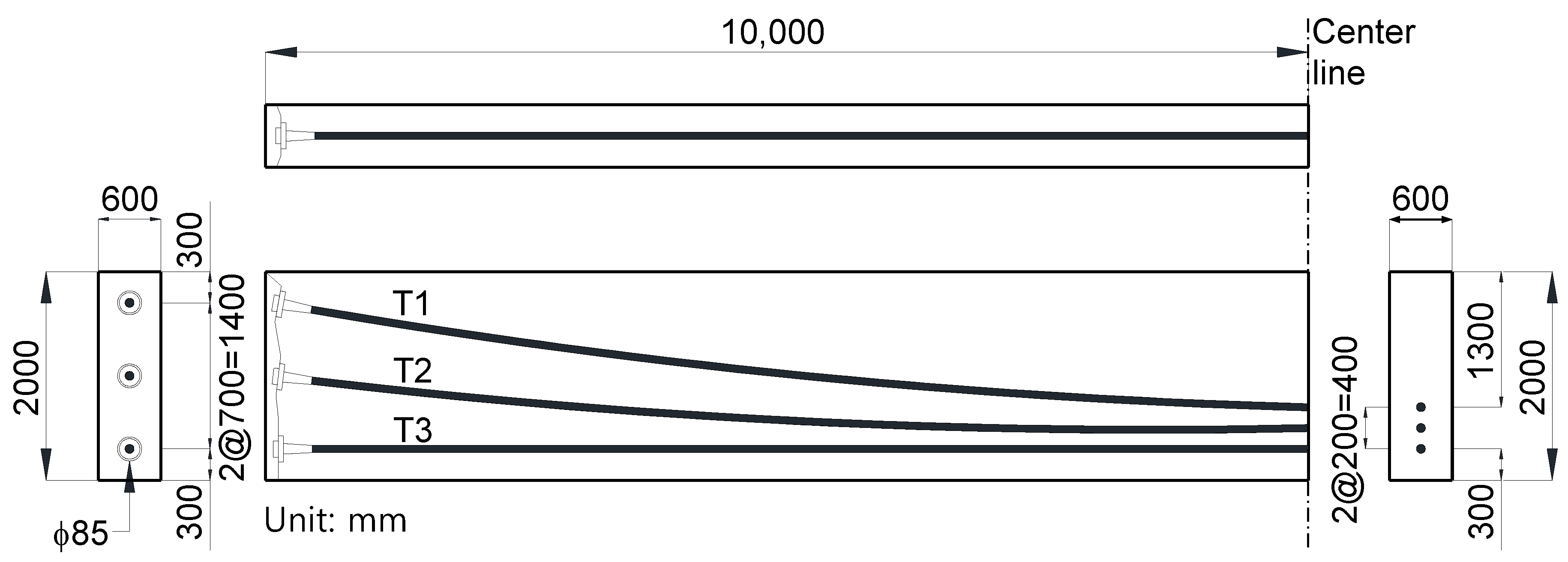
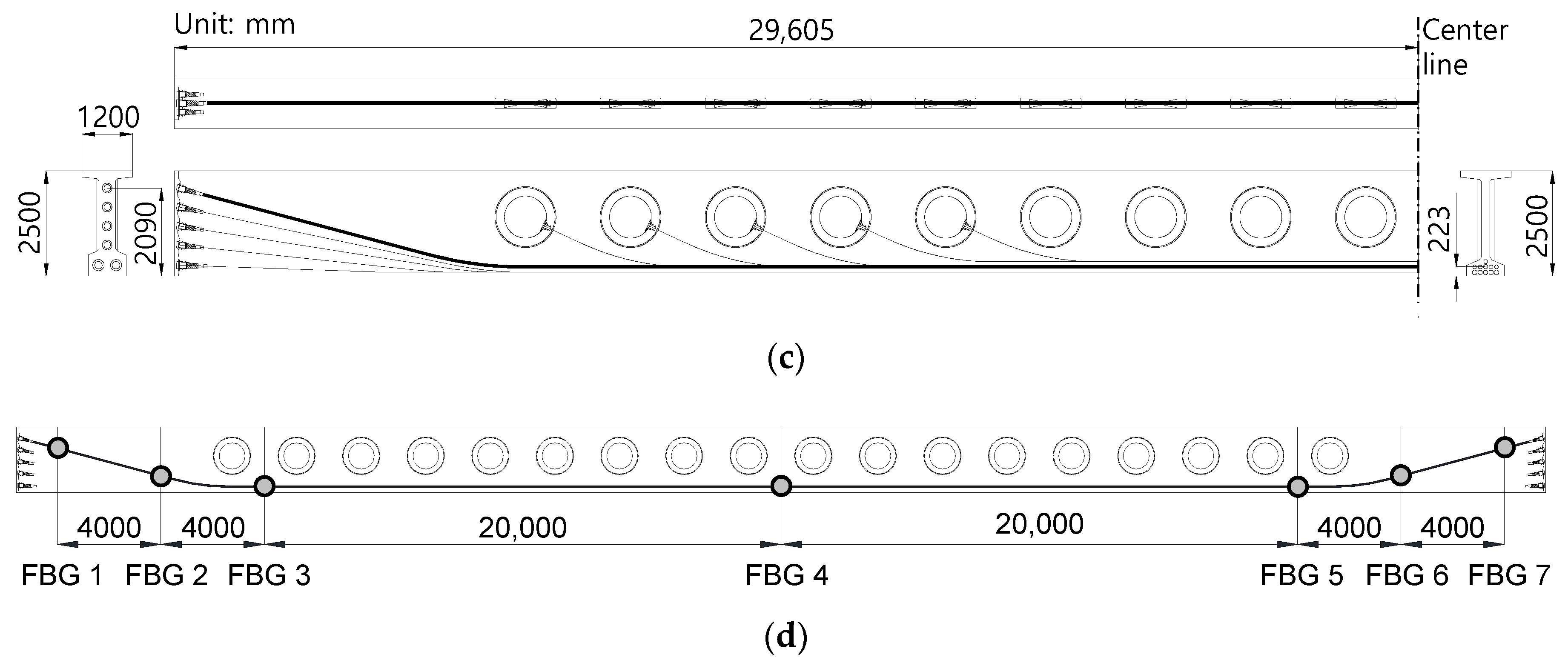
4.1. Full-Scale Specimen

Figure 3 shows the post-tensioned 20 m-long full-scale specimen which was fabricated to investigate the long-term characteristics of PF using Smart Strands. Three ducts denoted by T1, T2, and T3 in Figure 3 with different curvatures, including one straight duct of T3, were arranged and a total of 12 strands, each with a diameter of 15.2 mm and an ultimate tensile strength ( f p u ) of 1860 MPa, were inserted into each duct with a diameter of 85 mm. The strands in each duct were tensioned using a multi-strand jack up to 0.7 f p u at one end at a concrete age of 27 days when the concrete strength attained 30 MPa, which was considered in the calculation of E c . Then, all the ducts were grouted to bond the tendons. Three types of Smart Strand with three, five, and seven equally spaced FBGs, respectively, were fabricated and selectively inserted into each duct, together with regular strands. Figure 4 shows how the Smart Strands and regular strands were located in each anchor head, where the numbers indicate the number of FBGs.

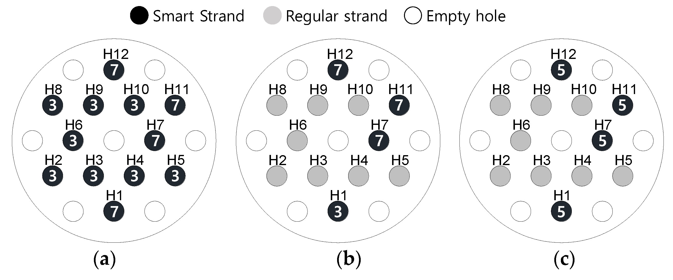
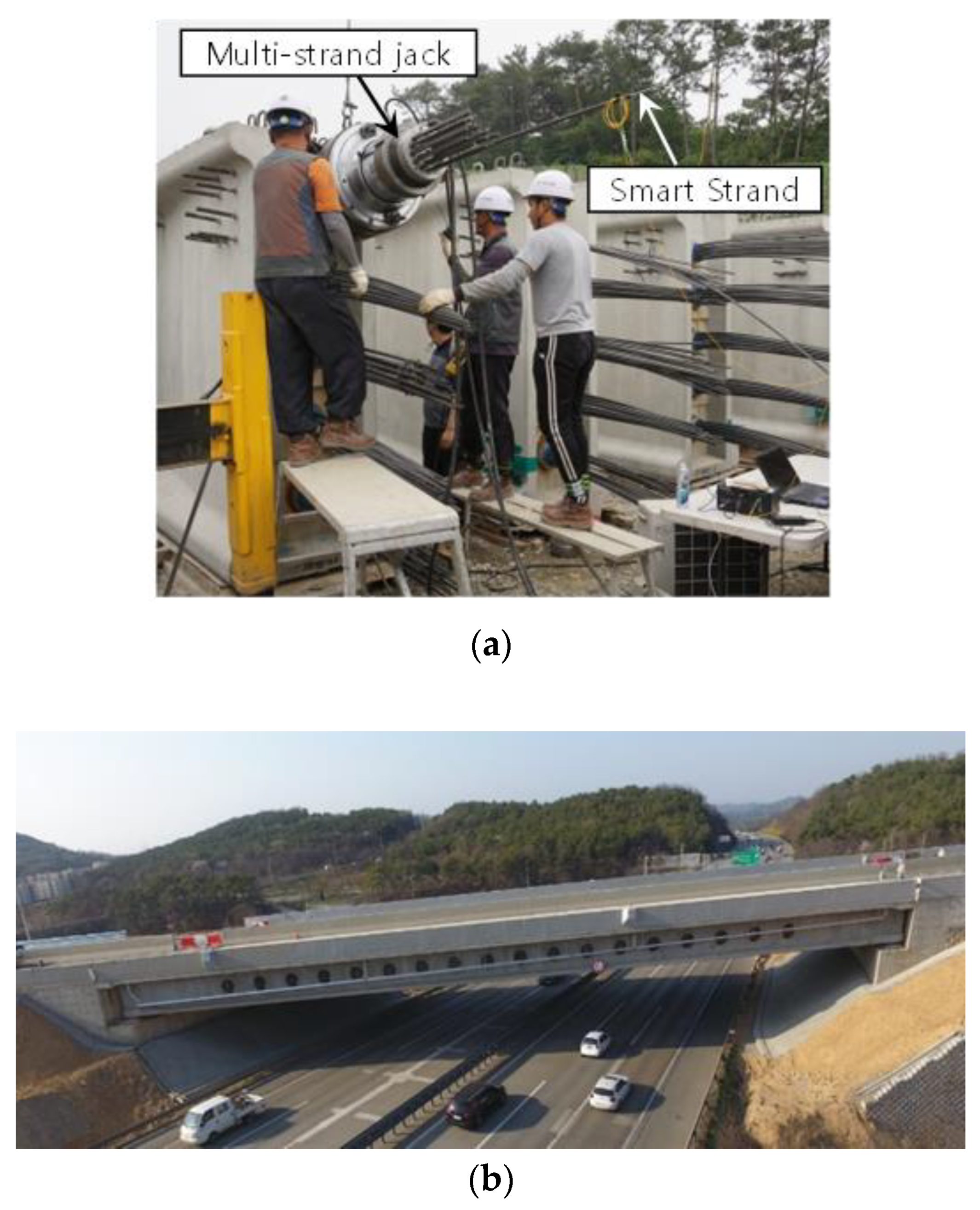
4.2. PSC Girder Bridge

Figure 5 shows the PSC girder bridge with a 60 m span, where one Smart Strand was applied to one of the six ducts arranged in one of the 10 girders for long-term monitoring. The girders of this bridge incorporate a series of holes in the web, which can enhance the aesthetics and reduce the self-weight, and have multi-stage prestressing, with the secondary tendons anchored at the holes [40]. The Smart Strand had seven FBGs and was inserted into the duct, together with 11 regular strands, as shown in Figure 5d. Six FBGs were concentrated near both ends of the girder because a wide range of variation in PF was anticipated there, whereas the remaining one FBG was located at the mid-span that is practically important in safety assessment. The strands were tensioned up to 0.675 f p u at the concrete age of 1 month using a multi-strand jack at both ends, after which the ducts were grouted. The diameter and f p u of the strands are the same as those used in the full-scale specimen and f c = 80 MPa.

5. Analysis of Long-Term Prestressing Force (PF)

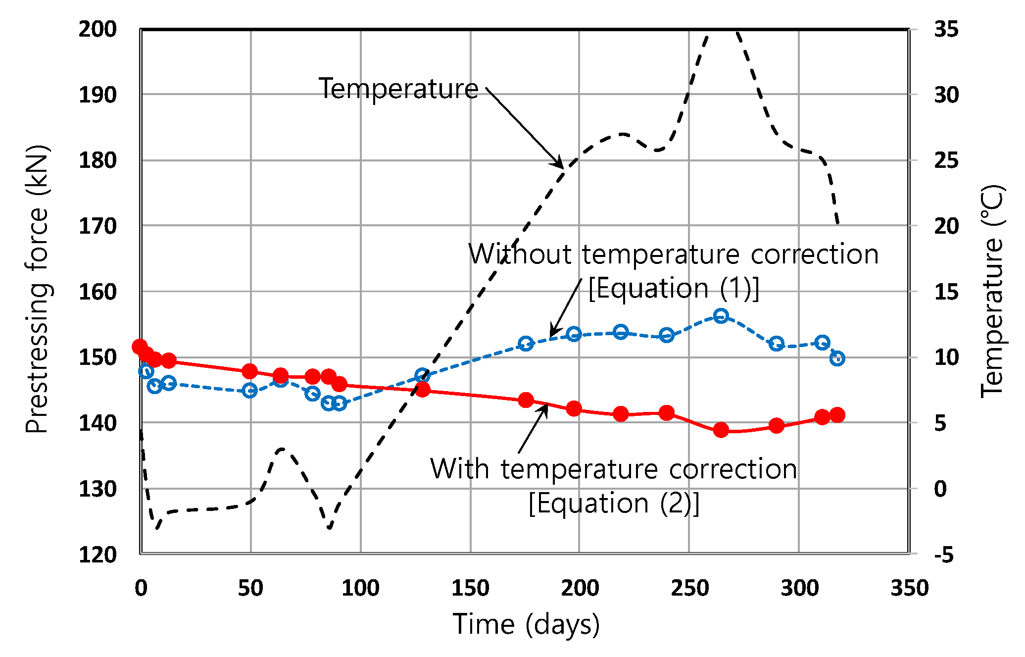
5.1. Importance of Temperature Correction

The PFs of the full-scale specimen and the PSC girder bridge were measured using Smart Strands for as long as possible, but the data measured for 318 days and 476 days after tensioning for the full-scale specimen and for the PSC girder bridge, respectively, were analyzed in this study. During the long-term measurement, the strains measured by sensors are affected by seasonal and daily temperature variations, and such temperature-dependent variation must be corrected or compensated for to derive the purely mechanical strain of interest that is directly related to stress. The correction can be accomplished by applying Equation (2) instead of Equation (1). Figure 6 compares the temporal PF variation before and after the temperature correction, which was measured in an FBG of a Smart Strand in the full-scale specimen. The temperatures were measured simultaneously when the wavelengths at FBGs were measured. The PF fluctuated in line with the trend of temperature variation without the correction, whereas consistent long-term prestress losses were obtained by applying the correction. Consequently, the following analyses are based on the temperature-corrected data. Abdel-Jaber and Glisic [9] also performed temperature compensation for the long-term strains obtained using FBGs. However, they did not rely on Equation (2), which was derived by taking the principles of FBGs into account, but simply applied a general temperature compensation procedure for concrete strain. This could be a potential problem due to the decreased accuracy of mechanical strain.

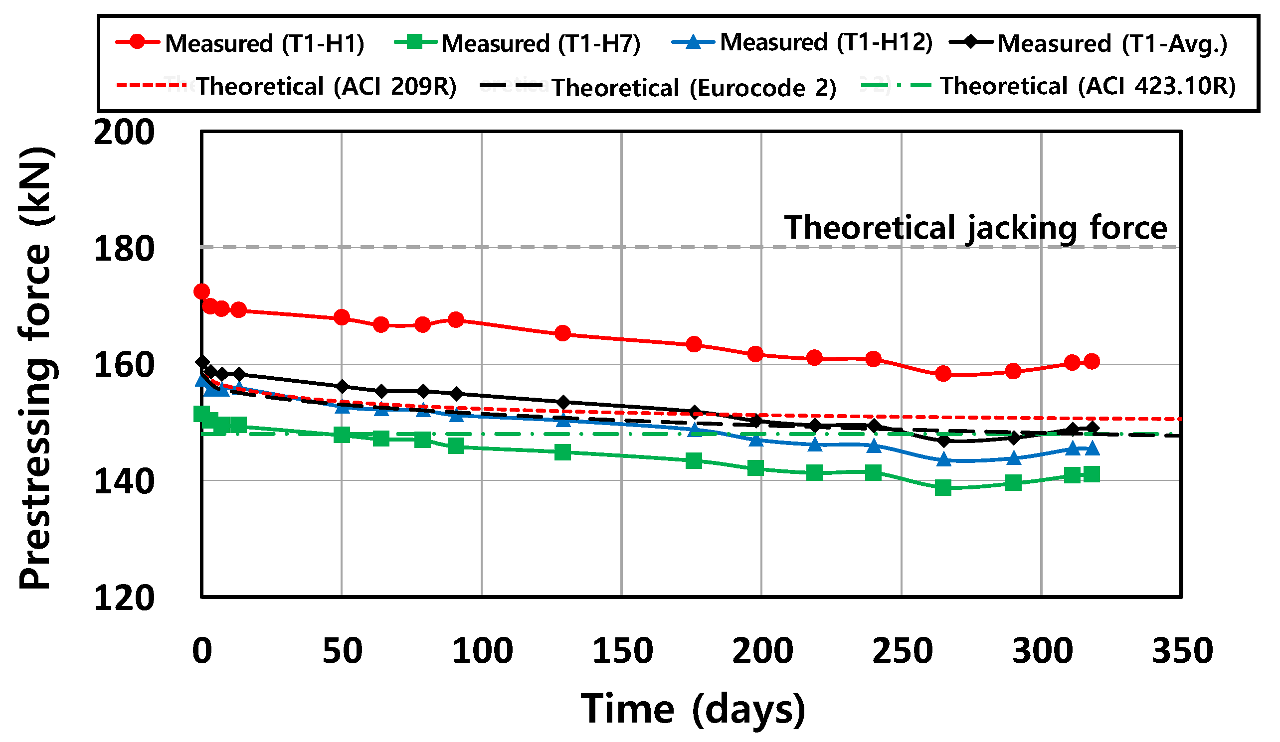
5.2. Long-Term Prestress Losses in the Full-Scale Specimen

Figure 7 representatively shows the distribution of PF in the Smart Strand of T1-H1 (refer to Figure 4) that varies at four time points: right after short-term losses of prestress in Figure 2, and 91, 198, and 318 days after tensioning. In the legend of Figure 7, “After short-term losses” indicates the beginning of the long-term losses and thus corresponds to “Tensioning + 0 days”. The measured distribution, which was obtained by connecting the PFs at FBGs (shown as bullets), was compared with that calculated by Eurocode 2 [38], which is one of the provisions analyzed in Figure 8. The theoretical values were calculated at 2-m intervals and interpolated. The theoretical jacking force of the strand, shown in Figure 7 and the following figures, was calculated by dividing the total jacking force measured in the multi-strand jack by the number of strands inserted into the corresponding duct. On the other hand, the actual jacking force in each strand was also measured using EM sensors. The measured jacking force of T1-H1 was 188 kN, which was higher than the theoretically estimated value of 180 kN. This aspect will be further analyzed below.
The theoretical PF can be obtained by subtracting the loss of PF (prestress loss multiplied by the area of a strand) from the original PF. Even the measured and theoretical distributions after the short-term losses do not completely agree with each other, because the short-term losses differed between the theoretical values obtained by predictive equations and measurement. However, the analysis of the PF distribution, based on the short-term losses, is beyond the scope of this study and will be covered in another study. The aforementioned difference between the measured and theoretical jacking forces is another factor that affects the subsequent long-term comparison. These intrinsic differences can be intentionally removed to make a reasonable comparison for long-term PFs, as is analyzed in Table 1, by introducing the difference of the PFs between two adjacent time steps. Note that the form of the PF distribution along the span of the specimen is unsymmetrical in both measurement and theory despite the symmetrical shape of the strand, as shown in Figure 7. Because all the strands were tensioned only at one end (left end), the unsymmetrical PF distribution is formed by the friction loss and anchorage-seating loss of Figure 2 and is maintained when subjected to other types of prestress losses.
It is apparent that the PFs were decreased over time by the long-term losses of prestress in both measurement and theory. Although the two approaches gave a similar decreasing trend, the decrement in each time step varied between the two, as shown in Figure 7 and Table 1. However, the total long-term losses, until 318 days after tensioning, are very comparable at 7.0% and 6.3% of the jacking force in measurement and theory, respectively, at the mid-span. Therefore, Eurocode 2 [38] made a reasonable estimation of the long-term prestress losses, as will be confirmed again by comparing with other provisions in Figure 8.
Figure 8 presents the PF variation at mid-span over time in both measurement and theory. H1, H7, and H12 of T1 in Figure 4 were representatively analyzed herein. Zero-day corresponds to the time after tensioning when the short-term losses had just occurred. The PFs measured at a specific time are different in three Smart Strands, including at the time of tensioning. This indicates that the PF of a strand can vary from strand to strand inside a duct due to the uneven interlocking between a strand and a wedge at the anchor head, although all the strands are tensioned simultaneously using a multi-strand jack. The PF variation of a strand in a duct was statistically analyzed by Cho et al. [19] Therefore, the averaged value of the PFs in the three Smart Strands was also provided in Figure 8 to reduce any bias.
The predictive equations for the long-term prestress losses induced by creep and shrinkage, that were introduced in Section 3, were compared with the measurements: ACI 209R [36], ACI 423.10R [34], and Eurocode 2 [38]. In contrast to ACI 209R and Eurocode 2, ACI 423.10R only suggests the ultimate creep and shrinkage losses without time function. However, relaxation loss was intentionally not considered in the equations to make a reasonable comparison with the Smart Strands, where the relaxation loss is not directly measured, as mentioned previously. Although the ultimate creep coefficient of ACI 209R is 2.35, it was reduced to 1.11 by incorporating such correction factors as loading age, ambient relative humidity (65%), and volume to surface ratio (231 mm). Likewise, the ultimate shrinkage strain of 780 × 10−6 m/m was reduced to 150 × 10−6 m/m by considering the correction factors, including relative humidity and volume to surface ratio, and by deducting the shrinkage that occurred before tensioning. Regarding Equation (10) of ACI 423.10R used for predicting ultimate shrinkage strain, the above three factors are already integrated into the equation. The detailed calculation of creep and shrinkage included in Equation (11) of Eurocode 2 involves a very complicated procedure, incorporating several correction factors, such as relative humidity, concrete compressive strength, loading age, type of cement, and notional size, which approximately corresponds to double the volume to surface ratio. The deduction of the shrinkage prior to tensioning was also separately considered.
Among the three equations considered, Eurocode 2 showed relatively good agreement with the averaged measurement values, partly because Equation (11) takes into account the long-term PF variation by applying the advanced technique of the age-adjusted effective modulus method (AEMM) [41] for more accurately calculating creep. Although ACI 209R also provided a good estimation for the trend of the long-term prestress losses, the latter half of the history after 180 days overestimated the actual PF, which is not desired for accurate and conservative design. On the other hand, the ultimate value of ACI 423.10R was very similar to the converged value of Eurocode 2, despite their different equations and parameters. Therefore, it would also be desirable to combine an appropriate time function with the ultimate creep coefficient and ultimate shrinkage strain of ACI 423.10R in order to obtain the time variation. The difference in the time function between ACI 209R and Eurocode 2 does not significantly affect the decreasing trend of the PF over time. The ultimate values of C u and ( ε s h ) u , together with a number of correction factors, greatly affected the long-term PF.

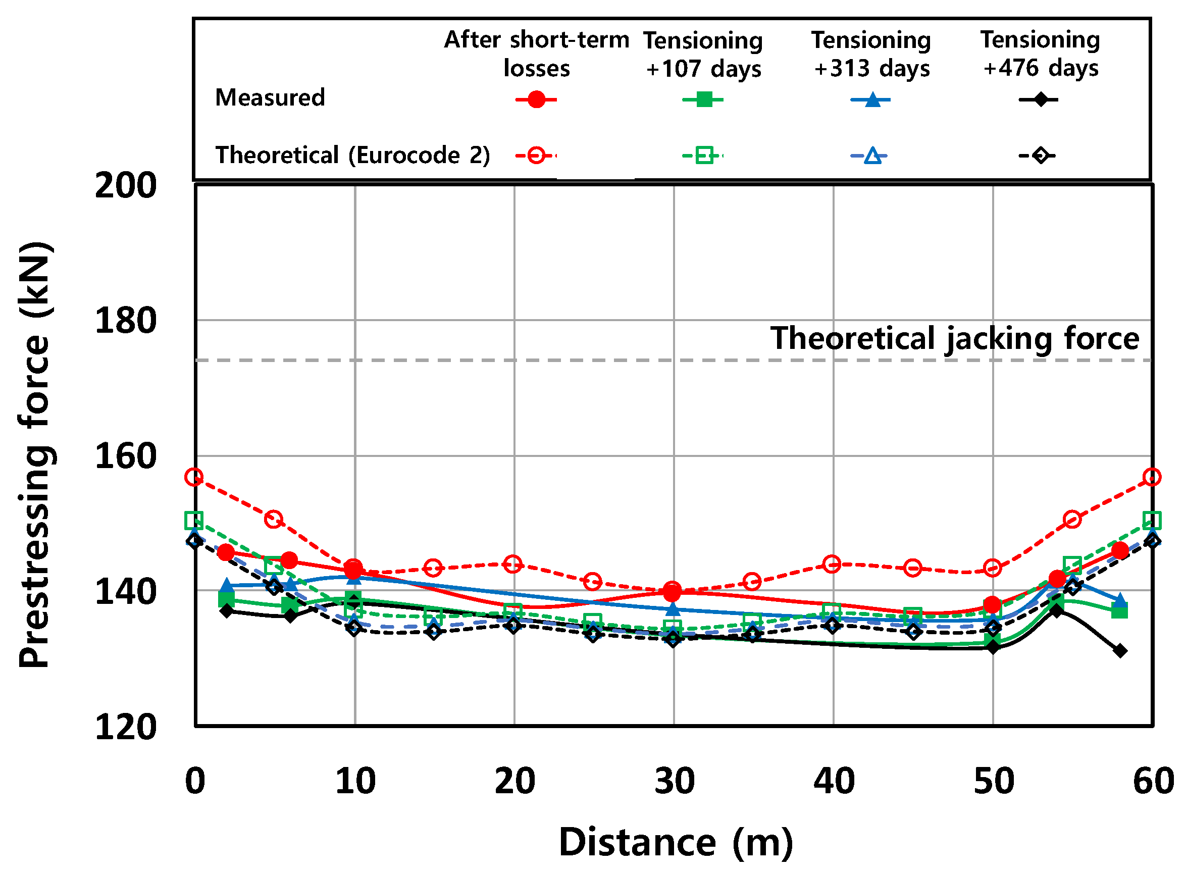
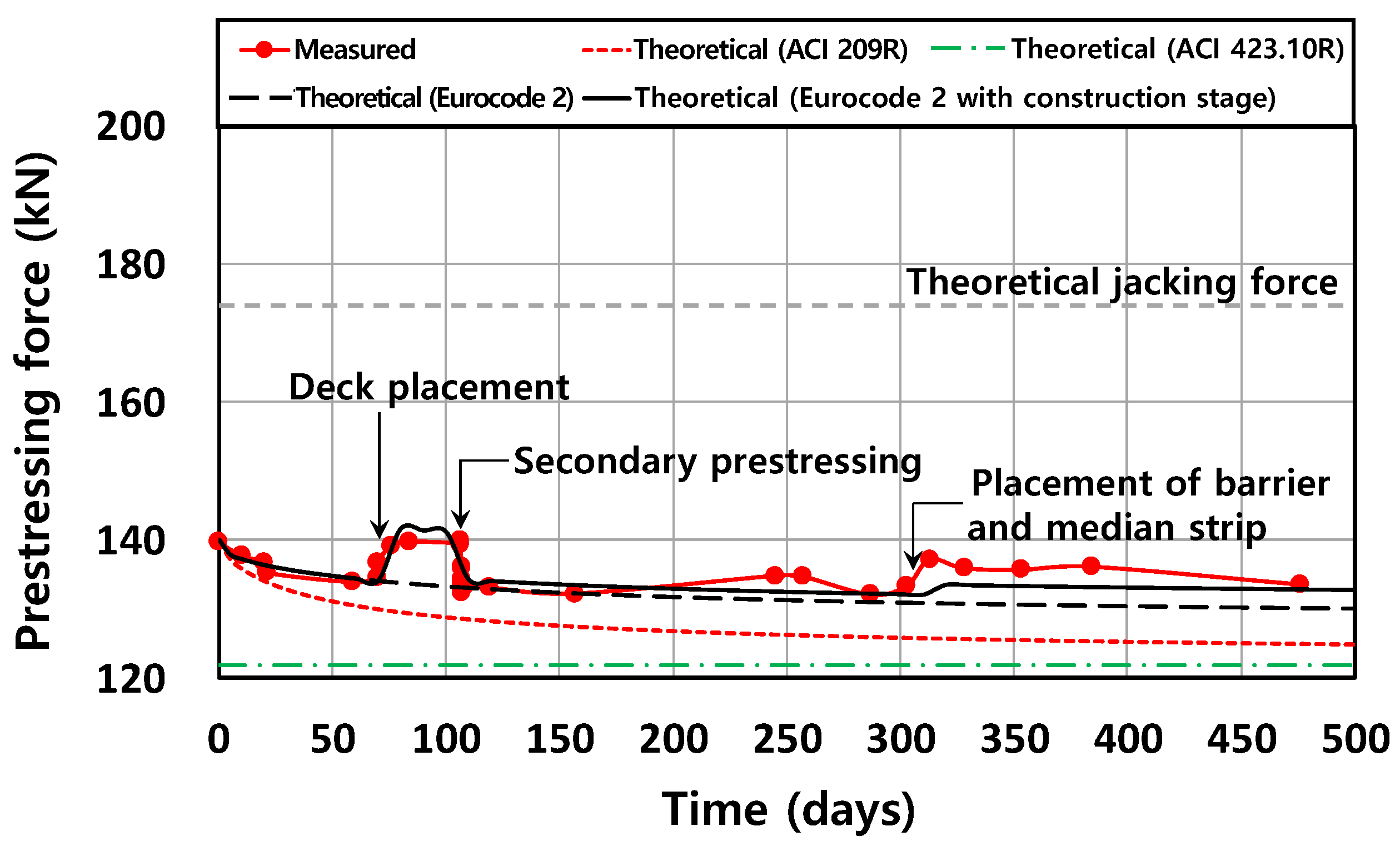
5.3. Long-Term Prestress Losses in the PSC Girder Bridge

Similar to the full-scale specimen, the theoretical estimation obtained by Eurocode 2 [38] and the measurement of PF were compared in Figure 9 at a few different time points. The bullets in the measured PF indicate the locations of FBGs, whereas the theoretical values were produced at 5-m intervals. Because the actual PF of each strand was not measured using an EM sensor, only the theoretical jacking force is presented.
Although both approaches produced a decreasing PF trend, the measured PF distribution was more irregular than that of the theory. This implies that the PF distribution is, in reality, more complex, and hence its theoretical estimation is more difficult. Despite the tensioning at both ends, the measured distribution does not assume the perfect symmetry that is theoretically predicted with respect to the center, and the strands seem to be entangled at the right end region, as implied by the irregularity of the distribution. The situation in the actual PSC girder bridge is further complicated by the effect of construction stages on the variation of the PF distribution; some construction stages can increase the PF, as opposed to the prestress losses. Therefore, the decreasing trend of the PF over time is not clear in some parts of the two graphs with consecutive times in Figure 9. This aspect will be further analyzed below. In the allowable stress design of PSC members, concrete stresses at the top fiber and the bottom fiber are adjusted to within a range of allowable stresses by the appropriate design of prestressing tendons. However, if the actual PF is significantly different from that estimated during the design, and if the marginal concrete stress is not sufficient, the concrete stresses can possibly exceed the allowable range, sometimes resulting in the cracking or crushing of concrete. The comparison shown in Figure 9 explains how and why this adverse outcome can occur in reality.
Figure 10 compares PFs at the mid-span between the predictive equations and the measurement. The figure suggests that several major construction stages caused significant PF fluctuations, in addition to the decreasing trend induced by long-term prestress losses. For example, when the additional dead loads were applied, including the deck and barrier, the PF tended to increase due to the deformation of the PSC girder and the accompanied elongation of the embedded prestressing tendon. On the contrary, the secondary prestressing, which is a special technique applied to extend the span [40], reduced the existing PF introduced at the primary prestressing stage due to elastic-shortening loss. Furthermore, the composite action of the girders and deck increases the complexity because of the change in cross-sectional constants for stress calculation and the difference in the long-term behavior of the girders and deck.
The same correction factors as those considered in the analysis of the full-scale specimen were applied to the predictive equations, including the volume to surface ratio (110 mm) of the girder. Consequently, the ultimate creep coefficient, 2.35, and the ultimate shrinkage strain, 780 × 10−6 m/m, were reduced to 1.23 and 259 × 10−6 m/m, respectively, in ACI 209R. Overall, Equation (11) of Eurocode 2 [38] was in good agreement with the measured values, similar to the full-scale specimen. Figure 10 also presents the theoretical PFs of Eurocode 2 with or without the additional consideration of the effect of a few major construction stages on the PF. However, the accurate evaluation of the PF, as affected by each construction stage, can be difficult because of the complex structural behavior in reality. In this respect, the responses of Smart Strands can also be utilized to assess the structural safety during construction and in service because they are critical in the structural health monitoring (SHM) of PSC structures. However, the predictive equations of ACI 209R [36] and ACI 423.10R [34] showed a relatively large difference from the measured PF, even though they provided a conservative estimation with a smaller PF than the measured value. The differences from the measured value at 476 days after tensioning were 0.6, 2.5, 6.5, and 8.8% in Eurocode 2 with and without construction stages, ACI 209R, and ACI 423.10R, respectively. These overall analysis results of the full-scale specimen and PSC girder bridge demonstrate that Eurocode 2 produced consistent and reliable estimation in both cases.
It is evident that a large portion of the long-term prestress losses occurred within a few months, while the remaining losses occurred gradually and subsequently. If the PF variation caused by the construction stages is excluded, approximately half of the total creep and shrinkage losses for 476 days occurred within approximately 1 month in the Smart Strand. The equations of ACI 209R and Eurocode 2 also exhibited a similar tendency. Therefore, the long-term prestress losses were concentrated at a relatively early concrete age in this study when compared to the results of Abdel-Jaber and Glisic [9], where half the long-term losses occurred within 6 months.

6. Conclusions

The correct design of the prestressing force (PF) distribution is very important to ensure the safety and serviceability of PSC structures. However, the prestress losses closely related to the PF distribution have generally been estimated using predictive equations specified in design codes or manuals, which were mostly derived from small-scale experiments. The validity of these equations at the scale of actual full-scale structures has not been sufficiently investigated because of the poor reliability and durability, and the difficulty in installation, when using conventional sensing technologies.
Therefore, Smart Strands with embedded fiber optic sensors were developed and applied to a 20 m-long full-scale specimen and a 60 m-long PSC girder bridge to investigate the characteristics of the PF distribution affected by long-term prestress losses. The measured data were compared with the theoretical values obtained by the predictive equations for long-term prestress losses that are specified in several design provisions. The results revealed that temperature correction or compensation is very important to obtain the PFs based on true mechanical strains, which are not affected by a seasonal or daily temperature variation in the long-term monitoring.
Although the two approaches of measurement and theory produced a similar long-term trend of the PF distribution, the difference between them varied depending on the design equations. The equation of Eurocode 2 to estimate the long-term prestress losses showed relatively good agreement with the measurement, when compared to that of ACI 209R and ACI 423.10R, for both the full-scale specimen and the actual PSC girder bridge. This can be attributed to the more refined form of the predictive equation of Eurocode 2 that addresses the time-dependency of the PF. The difference in the time function between ACI 209R and Eurocode 2 did not significantly affect the decreasing trend of the PF over time. The ultimate values of creep and shrinkage, together with a number of correction factors, greatly affected the long-term PF. In addition to the analysis of the long-term prestress losses, the Smart Strands also provided useful data in terms of the PF variation at each major stage during construction.
We expect our developed Smart Strand to be applied practically in PF measurement for the reasonable safety assessment and maintenance of structures, such as in structural health monitoring (SHM).

Author Contributions

Conceptualization, S.-H.K. and S.-J.J.; methodology, S.-H.K. and S.-J.J.; software, S.-H.K.; validation, S.-H.K. and S.-J.J.; formal analysis, S.-H.K.; investigation, S.-H.K. and S.-J.J.; resources, S.Y.P.; data curation, S.-H.K. and S.-J.J.; writing—original draft preparation, S.-H.K.; writing—review and editing, S.-J.J.; visualization, S.-H.K.; supervision, S.-J.J.; project administration, S.-J.J.; funding acquisition, S.Y.P. All authors have read and agreed to the published version of the manuscript.

Funding

This research received no external funding.

Acknowledgments

This research was supported by a grant from a Strategic Research Project (Smart Monitoring System for Concrete Structures Using FRP Nerve Sensors) funded by the Korea Institute of Civil Engineering and Building Technology. The efforts of Sung Tae Kim in the Korea Institute of Civil Engineering and Building Technology for preparing and monitoring the Smart Strands are also greatly appreciated.

Conflicts of Interest

The authors declare no conflict of interest.

References

  1. Potson, R.W.; Frank, K.H.; West, J.S. Enduring strength. Civ. Eng. ASCE 2003, 73, 58–63. [Google Scholar]
  2. Jeon, S.J.; Park, S.Y.; Kim, S.H.; Kim, S.T.; Park, Y.H. Estimation of friction coefficient using Smart Strand. Int. J. Concr. Struct. M 2015, 9, 369–379. [Google Scholar] [CrossRef] [Green Version]
  3. Kim, S.H.; Park, S.Y.; Park, Y.H.; Jeon, S.J. Friction characteristics of post-tensioning tendons in full-scale structures. Eng. Struct. 2019, 183, 389–397. [Google Scholar] [CrossRef]
  4. Russell, B.W.; Burns, N.H. Measured transfer lengths of 0.5 and 0.6 in. strands in pretensioned concrete. PCI J. 1996, 41, 44–65. [Google Scholar] [CrossRef]
  5. Jeon, S.J.; Shin, H.; Kim, S.H.; Park, S.Y.; Yang, J.M. Transfer lengths in pretensioned concrete measured using various sensing technologies. Int. J. Concr. Struct. M 2019, 13, 739–754. [Google Scholar] [CrossRef]
  6. Anderegg, P.; Brönnimann, R.; Meier, U. Reliability of long-term monitoring data. J. Civ. Struct. Health Monit. 2014, 4, 69–75. [Google Scholar] [CrossRef] [Green Version]
  7. Pessiki, S.; Kaczinski, M.; Wescott, H.H. Evaluation of effective prestress force in 28-year-old prestressed concrete bridge beams. PCI J. 1996, 41, 78–89. [Google Scholar] [CrossRef]
  8. Garber, D.B.; Gallardo, J.M.; Deschenes, D.J.; Bayrak, O. Experimental investigation of prestress losses in full-scale bridge girders. ACI Struct. J. 2015, 112, 553–564. [Google Scholar] [CrossRef] [Green Version]
  9. Abdel-Jaber, H.; Glisic, B. Monitoring of long-term prestress losses in prestressed concrete structures using fiber optic sensors. Struct. Health Monit. 2019, 18, 254–269. [Google Scholar] [CrossRef]
  10. Shing, P.B.; Kottari, A. Evaluation of Long-Term Prestress Losses in Post-Tensioned Box-Girder Bridges; Report No. SSRP-11/02; University of California, San Diego: La Jolla, CA, USA, 2011. [Google Scholar]
  11. Lundqvist, P.; Nilsson, L.O. Evaluation of prestress losses in nuclear reactor containments. Nucl. Eng. Des. 2011, 241, 168–176. [Google Scholar] [CrossRef]
  12. American Society for Testing and Materials (ASTM). Standard Specification for Low-Relaxation, Seven-Wire Strand for Prestressed Concrete; ASTM A416/A416M-18; ASTM International: West Conshohocken, PA, USA, 2018. [Google Scholar]
  13. Kim, J.T.; Yun, C.B.; Ryu, Y.S.; Cho, H.M. Identification of prestress-loss in PSC beams using modal information. Struct. Eng. Mech. 2004, 17, 467–482. [Google Scholar] [CrossRef]
  14. Rizzo, P. Ultrasonic wave propagation in progressively loaded multi-wire strands. Exp. Mech. 2006, 46, 297–306. [Google Scholar] [CrossRef]
  15. Washer, G.A.; Green, R.E.; Pond, R.B., Jr. Velocity constants for ultrasonic stress measurement in prestressing tendons. Res. Nondestruct. Eval. 2002, 14, 81–94. [Google Scholar] [CrossRef]
  16. Chaki, S.; Bourse, G. Stress level measurement in prestressed steel strands using acoustoelastic effect. Exp. Mech. 2009, 49, 673–681. [Google Scholar] [CrossRef]
  17. Chen, H.L.; Wissawapaisal, K. Measurement of tensile forces in a seven-wire prestressing strand using stress waves. J. Eng. Mech. 2001, 127, 599–606. [Google Scholar] [CrossRef]
  18. Fabo, P.; Jarosevic, A.; Chandoga, M. Health monitoring of the steel cables using the elasto-magnetic method. In Proceedings of the ASME 2002 International Mechanical Engineering Congress and Exposition, New Orleans, LA, USA, 17–22 November 2002; pp. 295–299. [Google Scholar]
  19. Cho, K.H.; Park, S.Y.; Cho, J.R.; Kim, S.T.; Park, Y.H. Estimation of prestress force distribution in the multi-strand system of prestressed concrete structures. Sensors 2015, 15, 14079–14092. [Google Scholar] [CrossRef] [Green Version]
  20. Deng, Y.; Liu, Y.; Chen, S. Long-term in-service monitoring and performance assessment of the main cables of long-span suspension bridges. Sensors 2017, 17, 1414. [Google Scholar] [CrossRef] [Green Version]
  21. Kim, J.M.; Kim, H.W.; Choi, S.Y.; Park, S.Y. Measurement of prestressing force in pretensioned UHPC deck using a fiber optic FBG sensor embedded in a 7-wire strand. J. Sens. 2016, 2016, 8634080. [Google Scholar] [CrossRef]
  22. Kim, J.M.; Kim, H.W.; Park, Y.H.; Yang, I.H.; Kim, Y.S. FBG sensors encapsulated into 7-wire steel strand for tension monitoring of a prestressing tendon. Adv. Struct. Eng. 2012, 15, 907–917. [Google Scholar] [CrossRef]
  23. Nellen, P.M.; Frank, A.; Broennimann, R.; Meier, U.; Sennhauser, U.J. Fiber optical Bragg grating sensors embedded in CFRP wires. SPIE Proc. 1999, 3670, 440–449. [Google Scholar]
  24. Zhou, Z.; He, J.; Chen, G.; Ou, J. A smart steel strand for the evaluation of prestress loss distribution in posttensioned concrete structures. J. Intel. Mater. Syst. Str. 2009, 20, 1901–1912. [Google Scholar] [CrossRef]
  25. Lan, C.; Zhou, Z.; Ou, J. Monitoring of structural prestress loss in RC beams by inner distributed Brillouin and fiber Bragg grating sensors on a single optical fiber. Struct. Control Hlth. 2014, 21, 317–330. [Google Scholar] [CrossRef]
  26. Perry, M.; Yan, Z.; Sun, Z.; Zhang, L.; Niewczas, P.; Johnston, M. High stress monitoring of prestressing tendons in nuclear concrete vessels using fibre-optic sensors. Nucl. Eng. Des. 2014, 268, 35–40. [Google Scholar] [CrossRef] [Green Version]
  27. Shen, S.; Wang, Y.; Ma, S.L.; Huang, D.; Wu, Z.H.; Guo, X. Evaluation of prestress loss distribution during pre-tensioning and post-tensioning using long-gauge fiber Bragg grating sensors. Sensors 2018, 18, 4106. [Google Scholar] [CrossRef] [PubMed] [Green Version]
  28. Magne, S.; Rougeault, S.; Vilela, M.; Ferdinand, P. State-of-strain evaluation with fiber Bragg grating rosettes: Application to discrimination between strain and temperature effects in fiber sensors. Appl. Opt. 1997, 36, 9437–9447. [Google Scholar] [CrossRef] [PubMed]
  29. Zhou, Z.; Ou, J. Techniques of temperature compensation for FBG strain sensors used in long-term structural monitoring. In Proceedings of the Asian Pacific Fundamental Problems of Opto- and Microelectronics (APCOM 2004), Khabarovsk, Russia, 13–16 September 2004; pp. 465–471. [Google Scholar]
  30. Pereira, G.; McGugan, M.; Mikkelsen, L.P. Method for independent strain and temperature measurement in polymeric tensile test specimen using embedded FBG sensors. Polym. Test. 2016, 50, 125–134. [Google Scholar] [CrossRef] [Green Version]
  31. Cho, K.; Kim, S.T.; Cho, J.R.; Park, Y.H. Analytical model of nonlinear stress-strain relation for a strand made of two materials. Materials 2017, 10, 1003. [Google Scholar]
  32. Nilson, A.H. Design of Prestressed Concrete, 2nd ed.; John Wiley & Sons, Inc.: Hoboken, NJ, USA, 1987; pp. 255–277. [Google Scholar]
  33. Zia, P.; Preston, H.K.; Scott, N.L.; Workman, E.B. Estimating prestress losses. Concr. Int. 1979, 1, 32–38. [Google Scholar]
  34. ACI-ASCE Committee 423. Guide to Estimating Prestress Loss; ACI 423.10R-16; American Concrete Institute (ACI): Farmington Hills, MI, USA, 2016. [Google Scholar]
  35. ACI Committee 318. Building Code Requirements for Structural Concrete; ACI 318-19; American Concrete Institute (ACI): Farmington Hills, MI, USA, 2019. [Google Scholar]
  36. ACI Committee 209. Prediction of Creep, Shrinkage, and Temperature Effects in Concrete Structures; ACI 209R-92; American Concrete Institute (ACI): Farmington Hills, MI, USA, 1997. [Google Scholar]
  37. Branson, D.E.; Kripanarayanan, K.M. Loss of prestress, camber and deflection of non-composite and composite prestressed concrete structures. PCI J. 1971, 16, 22–52. [Google Scholar] [CrossRef]
  38. European Committee for Standardization (CEN). Eurocode 2: Design of Concrete Structures—Part 1-1: General Rules and Rules for Buildings; EN 1992-1-1; CEN: Brussels, Belgium, 2004. [Google Scholar]
  39. Korea Road and Transportation Association (KRTA). Design Code for Highway Bridges (Limit State Design); KRTA: Seoul, Korea, 2015. [Google Scholar]
  40. Han, M.Y.; Jin, K.S.; Chang, D.H.; Kang, T.H.; Jeon, S.J. Effect of holes and segmentation on the structural behavior of a prestressed concrete girder. KSCE J. Civ. Eng. 2014, 18, 1711–1719. [Google Scholar] [CrossRef]
  41. Gilbert, R.I. Time Effects in Concrete Structures; Elsevier Science Publishers B. V.: Amsterdam, The Netherlands, 1988; pp. 64–68. [Google Scholar]
Figure 1. Configuration of a Smart Strand.
Applsci 10 04084 g001
Figure 2. Prestress losses.
Applsci 10 04084 g002
Figure 3. Post-tensioned full-scale specimen.
Applsci 10 04084 g003
Figure 4. Arrangement of strands in anchor heads: (a) T1, (b) T2, and (c) T3.
Applsci 10 04084 g004
Figure 5. Prestressed concrete (PSC) girder bridge: (a) Tensioning of strands, (b) view after completion, (c) arrangement of tendons, and (d) Smart Strand with fiber Bragg gratings (FBGs).
Applsci 10 04084 g005aApplsci 10 04084 g005b
Figure 6. Effect of temperature correction on the prestressing force (PF).
Applsci 10 04084 g006
Figure 7. Distribution of PFs in the full-scale specimen (T1-H1).
Applsci 10 04084 g007
Figure 8. PFs at mid-span in the full-scale specimen (T1-H1, H7, and H12).
Applsci 10 04084 g008
Figure 9. Distribution of PFs in the PSC girder bridge.
Applsci 10 04084 g009
Figure 10. PFs at mid-span in the PSC girder bridge.
Applsci 10 04084 g010
Table 1. PFs at the location of FBGs in the full-scale specimen (T1-H1).
Distance (m)14710131619
Measurement 2 (kN)
[difference (%)]
Tensioning188188188188188188188
After short-term losses167.2
[11.1] 1
168.8
[10.2]
166.5
[11.4]
172.4
[8.3]
172.5
[8.2]
167.5
[10.9]
168.4
[10.4]
Tensioning + 91 days162.6
[2.7]
165.3
[2.1]
163.6
[1.8]
167.5
[2.8]
167.6
[2.8]
163.6
[2.3]
164.1
[2.6]
Tensioning + 198 days155.9
[4.1]
159.4
[3.6]
157.9
[3.5]
161.7
[3.5]
161.9
[3.5]
157.8
[3.6]
158.0
[3.7]
Tensioning + 318 days155.3
[0.4]
158.7
[0.4]
156.9
[0.6]
160.3
[0.8]
160.9
[0.6]
156.7
[0.7]
157.1
[0.6]
Theory 3
(kN)
[difference (%)]
Tensioning180180180180180180180
After short-term losses151.4
[15.9]
154.1
[14.4]
155.8
[13.5]
158.2
[12.1]
158.6
[11.9]
157.2
[12.7]
154.9
[13.9]
Tensioning + 91 days145.9
[3.6]
148.6
[3.5]
149.8
[3.8]
151.8
[4.1]
152.6
[3.8]
151.6
[3.5]
149.3
[3.6]
Tensioning + 198 days143.9
[1.4]
146.6
[1.3]
147.8
[1.4]
149.7
[1.4]
150.5
[1.4]
149.6
[1.3]
147.2
[1.3]
Tensioning + 318 days142.5
[1.0]
145.3
[0.9]
146.4
[1.0]
148.2
[1.0]
149.1
[0.9]
148.3
[0.9]
145.8
[1.0]
1 Square bracket indicates the difference of PF from previous time step (%); 2 T1-H1; 3 Eurocode 2.

