A Study on the Amplitude Comparison Monopulse Algorithm

Abstract

This paper presents two amplitude comparison monopulse algorithms and their covariance prediction equation. The proposed algorithms are based on the iterated least-squares estimation method and include the conventional monopulse algorithm as a special case. The proposed covariance equation is simple but predicts RMS errors very accurately. This equation quantitatively states estimation accuracy in terms of major parameters of amplitude comparison monopulse radar, and is also applicable to the conventional monopulse algorithm. The proposed algorithms and covariance prediction equations are validated by the numerical simulations with 100,000 Monte Carlo runs.

1. Introduction

Monopulse radar operates by comparing signal returns of four squinted beams steered around the expected target direction [1]. It is classified as amplitude comparison monopulse and phase comparison monopulse, and amplitude comparison monopulse is the most commonly used method, which detects azimuth and elevation deviation errors from the center of the track axis by comparing the amplitudes of the signal returns.

Many methods have been proposed to improve the performance of monopulse algorithms in the literature [2,3,4,5,6,7,8,9]. Hofstetter and DeLong [2] dealt with the problem of detecting and estimating the unknown angular position of the target observed simultaneously by controlling the number of antennas in the amplitude comparison monopulse radar, where the method is derived using a generalized likelihood ratio test. Sim et al. [3] carried out a performance analysis according to antenna spacing using the phase comparison monopulse algorithm and proposed an efficient nonlinear antenna array based on the analysis results. Han et al. [4] showed the effect of the functional variables of the monopulse radar on angular tracking performance. An and Lee [5] showed the performance of amplitude comparison monopulse through simulation-based MSE (mean-square error) comparison with analytic MSE obtained by linearly approximating the nonlinear estimation equations. Jacovitti [6] carried out a performance analysis on the monopulse receivers in the secondary surveillance radar where the internal sources of error are considered. This paper discussed the general performance of the receiver of the monopulse radar where Gaussian noise is applied in the environment. Chen and Sheng [7] analyzed the performance of an angle measurement of the monopulse radar with reception non-consistency. This paper showed that the performance of the angle measurement depends not only on the algorithm but also on the reception consistency. Mosca [8] discussed the estimation problem of the angle of arrival in thermal noise-applied amplitude comparison monopulse radar in terms of the coherency of pulse returns. In [9], a novel methodology that overcomes the limitation of difference beam aided detection was proposed.

While many monopulse algorithms are proposed so far to improve the estimation performance, most of them do not have clear relationships with the conventional algorithm, and only few conduct the performance analysis under the presence of measurement noise. Therefore, it is difficult to evaluate their performance improvement over the conventional algorithm under the measurement noise presence. Although some papers deal with formal noise analysis on the conventional algorithm, it is extremely complex, and no useful information comes from it.

Motivated by these observations, this paper presents least-squares-based monopulse algorithms and a novel covariance prediction equation. The proposed algorithms have an iterative process that incrementally improves the accuracy of the conventional algorithm. It is shown that the conventional monopulse algorithm is a special case of the proposed algorithms with the first iterative step. The proposed covariance equation is simple but predicts very accurately the covariance of the estimated target location under the presence of measurement noise. This equation is independent of the measurement signal, and thus can be used to predict the performance of the monopulse algorithms before the algorithms are actually performed. This equation is also applicable to conventional monopulse algorithms, and quantitatively states estimation accuracy in terms of the major parameters of amplitude comparison monopulse radar.

It is also important in in electronic warfare systems to predict the performance of amplitude comparison monopulse in terms of major parameters since intercepted signals from different types of radars are very often noisy and change depending on the mission being carried out and the task being performed [10,11].

This paper is organized as follows. In Section 2, the conventional amplitude comparison monopulse algorithm is explained. In Section 3, two least-squares-based monopulse algorithms are proposed. Section 4 discusses the relationships between the proposed and the conventional algorithms. In Section 5, a novel covariance equation is proposed as a performance prediction measure. In Section 6, numerical simulations are performed to evaluate the proposed algorithm and covariance equation. Conclusions are given in Section 6.

2. Conventional Amplitude Comparison Monopulse Algorithm

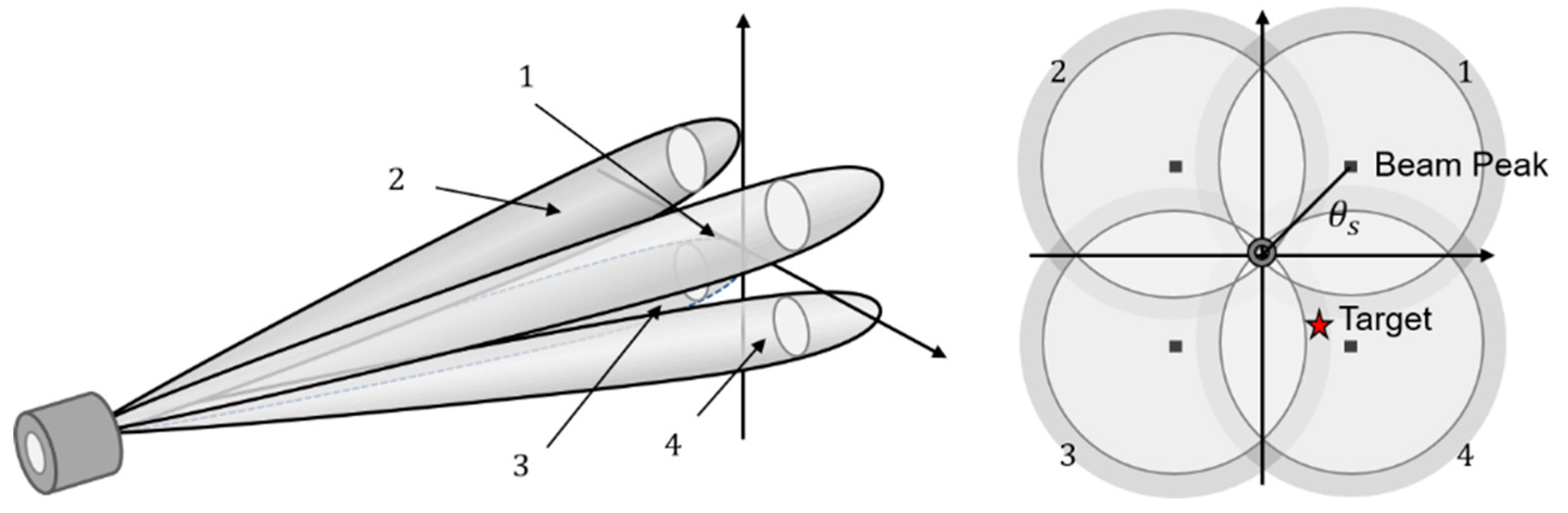
Measurement of the target direction angle or target location is required for target tracking. Amplitude comparison monopulse radar operates by comparing the amplitude of signal returns of four squinted sub-beams steered symmetrically around the expected target direction as shown in Figure 1 [1]. The sum, horizontal difference, and vertical difference channels of the incoming signal are used to estimate target location, which is represented by the azimuth and elevation angle deviations in the track axis.

Each antenna pattern can be modeled near the center of the track axis as a squinted Gaussian beam. Each one-way voltage gain function is given by

$$g\left(\theta \right)=g_0\exp \left(-2{\left(\frac{\theta }{{\theta }_{3dB}}\right)}^2\log 2\right)$$

(1)

where $\theta$ is the total angle from the target location to the beam peak, ${\theta }_{3dB}$ is the beam width, and $g_0$ is the gain at the beam peak [12].

The total angle, $\theta$, can be computed from the target location defined in Figure 2, which presents the field of view as seen from the monopulse radar.

For a beam with its maximum in quadrant 1, the target location from the beam peak can be written in terms of azimuth and elevation angle deviations (${\theta }_{az}, {\theta }_{el}$) as

$${\theta }^2={\left(\frac{{\theta }_s}{\sqrt{2}}-{\theta }_{az}\right)}^2+{\left(\frac{{\theta }_s}{\sqrt{2}}-{\theta }_{el}\right)}^2$$

(2)

and the quadrant 1 voltage gain is then

$$g_1\left(\theta \right)=g_1\left({\theta }_{az},{\theta }_{el}\right)=g_0\exp \left[-2\left(\frac{{\left(\frac{{\theta }_s}{\sqrt{2}}-{\theta }_{az}\right)}^2+{\left(\frac{{\theta }_s}{\sqrt{2}}-{\theta }_{el}\right)}^2}{{\theta }_{3dB}^2}\right)\log 2\right]$$

(3)

where ${\theta }_s$ is the squint angle of the antenna. Using the above gain functions and a received signal voltage of amplitude A, the so-called pseudorange equations are given as follows:

$$\left[\begin{array}{c}{s}_1\\ \begin{array}{c}{s}_2\\ \begin{array}{c}{s}_3\\ s_4\end{array}\end{array}\end{array}\right]=A\left[\begin{array}{c}{g}_1\left({\theta }_{az},{\theta }_{el}\right)\\ \begin{array}{c}{g}_2\left({\theta }_{az},{\theta }_{el}\right)\\ g_3\left({\theta }_{az},{\theta }_{el}\right)\\ g_4\left({\theta }_{az},{\theta }_{el}\right)\end{array}\end{array}\right]+\left[\begin{array}{c}{n}_1\\ \begin{array}{c}{n}_2\\ \begin{array}{c}{n}_3\\ n_4\end{array}\end{array}\end{array}\right]$$

(4)

where $s_i$ is the measurement signal of $i$-th quadrant, which is contaminated by the measurement noise $n_i$. Here, $s_i$ can be considered as pseudorange since it is a function of geometrical distance weighted by the antenna gain.

The conventional amplitude comparison monopulse algorithm for estimating azimuth and elevation angle deviations is briefly explained in the next few paragraphs [4,5,12].

Assuming that ${\theta }_{az}^2+{\theta }_{el}^2\approx 0$, the quadrant 1 voltage gain is simplified as follows:

$$g_1\left(\theta \right)=g_1\left({\theta }_{az},{\theta }_{el}\right) \approx g\left({\theta }_s\right) \exp \left[2\sqrt{2} \left(\frac{{\theta }_s}{{\theta }_{3dB}}\right) \left(\frac{{\theta }_{az}+{\theta }_{el}}{{\theta }_{3dB}}\right)\log 2\right]$$

(5)

If a monopulse error slope coefficient is defined as

$$k_m=2\sqrt{2} \left(\frac{{\theta }_s}{{\theta }_{3dB}}\right)\log 2$$

(6)

then, voltage gain for the beam in quadrant 1 should be

$$g_1\left({\theta }_{az},{\theta }_{el}\right)=g\left({\theta }_s\right) \exp \left[k_m \left(\frac{{\theta }_{az}+{\theta }_{el}}{{\theta }_{3dB}}\right)\right]\approx g_0\left[1+\frac{k_m}{{\theta }_{3dB}} \left({\theta }_{az}+{\theta }_{el}\right)\right]$$

(7)

assuming $k_m\left(\frac{{\theta }_{az}+{\theta }_{el}}{{\theta }_{3dB}}\right)\ll 1$.

Under the assumption that all patterns are in phase, the gain functions of the antenna patterns directed into the other quadrants are approximately computed as

$$g_1\left({\theta }_{az},{\theta }_{el}\right)\approx g_0\left[1+\frac{k_m}{{\theta }_{3dB}} \left({\theta }_{az}+{\theta }_{el}\right)\right]$$

(8)

$$g_2\left({\theta }_{az},{\theta }_{el}\right)\approx g_0\left[1+\frac{k_m}{{\theta }_{3dB}} \left(-{\theta }_{az}+{\theta }_{el}\right)\right]$$

(9)

$$g_3\left({\theta }_{az},{\theta }_{el}\right)\approx g_0\left[1-\frac{k_m}{{\theta }_{3dB}} \left({\theta }_{az}+{\theta }_{el}\right)\right]$$

(10)

$$g_4\left({\theta }_{az},{\theta }_{el}\right)\approx g_0\left[1+\frac{k_m}{{\theta }_{3dB}} \left({\theta }_{az}-{\theta }_{el}\right)\right]$$

(11)

Then, the sum ($\mathsf{\Sigma })$, horizontal difference (${\mathsf{\Delta }}_{az}$), and vertical difference (${\mathsf{\Delta }}_{el}$) voltages are calculated by

$$\mathsf{\Sigma }=A\left[g_1+g_2+g_3+g_4\right]=4A{g}_0$$

(12)

$${\mathsf{\Delta }}_{az}=A\left[g_1+g_4-\left(g_2+g_3\right)\right]=4A{g}_0\frac{k_m}{{\theta }_{3dB}}{\theta }_{az}$$

(13)

$${\mathsf{\Delta }}_{el}=A\left[g_1+g_2-\left(g_3+g_4\right)\right]=4A{g}_0\frac{k_m}{{\theta }_{3dB}}{\theta }_{el}$$

(14)

Therefore, the azimuth and elevation angle deviations can be estimated as

$${\widehat{\theta }}_{az}^c=\frac{{\mathsf{\Delta }}_{az}}{\mathsf{\Sigma }}\frac{{\theta }_{3dB}}{k_m}$$

(15)

$${\widehat{\theta }}_{el}^c=\frac{{\mathsf{\Delta }}_{el}}{\mathsf{\Sigma }}\frac{{\theta }_{3dB}}{k_m}$$

(16)

where ${\widehat{\theta }}_{az}^c$ and ${\widehat{\theta }}_{el}^c$ are the estimates of azimuth and elevation angle deviations, respectively, which represent the unknown target location estimate.

3. Least-Squares-Based Amplitude Comparison Monopulse Algorithm

3.1. Full Measurement-Based Algorithm

We can solve the estimation problems of azimuth and elevation angle deviations by first linearizing the pseudorange Equation (4), then using the familiar least-squares method.

Let the vector of measured signals be $S={\left[s_1 s_2 s_3 s_4 \right]}^T$; then, Equation (4) can be written in matrix form compactly as follows:

$$S=A{h}_{full}\left({\theta }_{az},{\theta }_{el}\right)+n$$

(17)

where $h_{full}={\left[g_1 g_2 g_3 g_4 \right]}^T$, and $n={\left[n_1 n_2 n_3 n_4 \right]}^T$.

If we expand the pseudorange Equation (17) in Taylor series about some nominal values $\left({\theta }_{az0},{\theta }_{el0}\right)$, and ignore the second and higher order terms, then this equation becomes

$$S\approx A{h}_{full}\left({\theta }_{az0},{\theta }_{el0}\right)+A\frac{\partial h_{full}}{\partial {\theta }_{az}}\left({\theta }_{az}-{\theta }_{az0}\right)+A\frac{\partial h_{full}}{\partial {\theta }_{el}}\left({\theta }_{el}-{\theta }_{el0}\right)+n$$

(18)

Note that the partial derivatives in the above expression are computed using nominal values $\left({\theta }_{az0},{\theta }_{el0}\right)$. The residual signal $\mathsf{\delta }S$ is defined as the difference between the actual signal and the signal computed using nominal values:

$$\begin{gathered} \delta S=S-A{h}_{full}\left({\theta }_{az0},{\theta }_{el0}\right) \\ \approx A\frac{\partial h_{full}}{\partial {\theta }_{az}}\delta {\theta }_{az}+A\frac{\partial h_{full}}{\partial {\theta }_{el}}\delta {\theta }_{el}+n \end{gathered}$$

(19)

where $\delta {\theta }_{az}={\theta }_{az}-{\theta }_{az0}$ and $\delta {\theta }_{el}={\theta }_{el}-{\theta }_{el0}$.

This equation can be written in four scalar equations in matrix form:

$$\left[\begin{array}{c}\delta s_1\\ \begin{array}{c}\delta s_2\\ \begin{array}{c}\delta s_3\\ \delta s_4\end{array}\end{array}\end{array}\right]\approx \frac{4\log 2 }{{\theta }_{3dB}^2}A \left[\begin{array}{cc} \left(\frac{{\theta }_s}{\sqrt{2}}-{\theta }_{az}\right) g_1& \left(\frac{{\theta }_s}{\sqrt{2}}-{\theta }_{el}\right) g_1\\ -\left(\frac{{\theta }_s}{\sqrt{2}}+{\theta }_{az}\right) g_2& \left(\frac{{\theta }_s}{\sqrt{2}}-{\theta }_{el}\right) g_2\\ \begin{array}{c}-\left(\frac{{\theta }_s}{\sqrt{2}}+{\theta }_{az}\right) g_3\\ \left(\frac{{\theta }_s}{\sqrt{2}}-{\theta }_{az}\right) g_4\end{array}& \begin{array}{c}-\left(\frac{{\theta }_s}{\sqrt{2}}+{\theta }_{el}\right) g_3\\ -\left(\frac{{\theta }_s}{\sqrt{2}}+{\theta }_{el}\right) g_4\end{array}\end{array}\right]\left[\begin{array}{c}\delta {\theta }_{az}\\ \delta {\theta }_{el}\end{array}\right]+\left[\begin{array}{c}{n}_1\\ \begin{array}{c}{n}_2\\ \begin{array}{c}{n}_3\\ n_4\end{array}\end{array}\end{array}\right]$$

(20)

which can be written in symbolic form as

$$\delta S\approx H_{full} \delta \theta +n$$

(21)

This equation expresses a linear relationship between the residual signals $\delta S$ and the unknown correction to angle deviations $\delta \theta$. Note that each row of $H_{full}$ is shown to be purely a gain-weighted direction vector to each of the beam peaks, as observed from the unknown target location in Figure 3.

Let us consider a solution for the linearized pseudorange equation, denoted as $\delta {\widehat{\theta }}^{full}$. The estimated residual $e$ is defined as the difference between the measured signal and its estimate. Using the linearized form of the pseudorange equations and ignoring measurement noise, the estimated residual is

$$e=\delta S-H_{full}\delta {\widehat{\theta }}^{full}$$

(22)

The least-squares solution can be found by minimizing the following functional:

$$J\left(\delta {\widehat{\theta }}^{full}\right)=\frac{1}{2}{e}^{T}e$$

(23)

Then, the solution is

$$\delta {\widehat{\theta }}^{full}={\left(H_{full}^T{H}_{full}\right)}^{-1}{H}_{full}^T\delta S$$

(24)

This equation assumes that the inverse to $H_{full}^T{H}_{full}$ exists, which is always true unless voltage gains are zero because of the beam peak and unknown target location geometries.

Iterated least-squares estimation starts with setting the initial gradient of Equation (24) with respect to ${\theta }_{az0}=0$ and ${\theta }_{el0}=0$ and repeatedly performs the following update until convergence or up to a certain number of iterations:

$$\begin{array}{c}{\widehat{\theta }}^{full}={\theta }_0+\delta {\widehat{\theta }}^{full}\\ {\theta }_0 \leftarrow {\widehat{\theta }}^{full}\end{array}$$

(25)

3.2. Sum-Difference Measurement-Based Algorithm

We can solve the estimation problem of azimuth and elevation angle deviations using the sum ($\mathsf{\Sigma })$, horizontal difference (${\mathsf{\Delta }}_{az}$), and vertical difference (${\mathsf{\Delta }}_{el}$) signals, which are used in the conventional monopulse algorithm. Utilizing these signals is more useful because the same circuitry as the conventional one can be used.

The measurement equations can be constructed as follows:

$$\begin{array}{c}\mathsf{\Sigma }=A\left[g_1+g_2+g_3+g_4\right]+n_1+n_2+n_3+n_4\\ {\mathsf{\Delta }}_{az}=A\left[g_1+g_4-\left(g_2+g_3\right)\right]+n_1+n_4-n_2-n_3\\ {\mathsf{\Delta }}_{el}=A\left[g_1+g_2-\left(g_3+g_4\right)\right]+n_1+n_2-n_3-n_4\end{array}$$

(26)

Let the vector of the measured signals be $Z={\left[\begin{array}{ccc}\mathsf{\Sigma }& {\mathsf{\Delta }}_{az}& {\mathsf{\Delta }}_{el}\end{array} \right]}^T$; then, Equation (26) can be written in matrix form compactly as follows:

$$Z=A{h}_{sd}\left({\theta }_{az},{\theta }_{el}\right)+Bn$$

(27)

where

$$h_{sd}=\left[\begin{array}{c}{g}_1+g_2+g_3+g_4\\ g_1+g_4-\left(g_2+g_3\right)\\ g_1+g_2-\left(g_3+g_4\right)\end{array}\right], B=\left[\begin{array}{ccc}1& 1& \begin{array}{cc}1& 1\end{array}\\ 1& -1& \begin{array}{cc}-1& 1\end{array}\\ 1& 1& \begin{array}{cc}-1& -1\end{array}\end{array}\right]$$

(28)

Similar to Section 3.1, by Taylor series expansion about some nominal values $\left({\theta }_{az0},{\theta }_{el0}\right)$, the linearized measurement equation becomes

$$\begin{gathered} \left[\begin{array}{c}\delta \mathsf{\Sigma }\\ \delta {\mathsf{\Delta }}_{az}\\ \delta {\mathsf{\Delta }}_{el}\end{array}\right]\approx B\left[\begin{array}{c}{n}_1\\ \begin{array}{c}{n}_2\\ \begin{array}{c}{n}_3\\ n_4\end{array}\end{array}\end{array}\right] \\ +\frac{4 \log 2 }{{\theta }_{3dB}^2}A\left[\begin{array}{cc}\left(\frac{{\theta }_s}{\sqrt{2}}-{\theta }_{az}\right)(g_1+g_4)-\left(\frac{{\theta }_s}{\sqrt{2}}+{\theta }_{az}\right)(g_2+g_3)& \left(\frac{{\theta }_s}{\sqrt{2}}-{\theta }_{el}\right)(g_1+g_2)-\left(\frac{{\theta }_s}{\sqrt{2}}+{\theta }_{el}\right)(g_3+g_4)\\ \left(\frac{{\theta }_s}{\sqrt{2}}-{\theta }_{az}\right)(g_1+g_4)+\left(\frac{{\theta }_s}{\sqrt{2}}+{\theta }_{az}\right)(g_2+g_3)& \left(\frac{{\theta }_s}{\sqrt{2}}-{\theta }_{el}\right)(g_1-g_2)+\left(\frac{{\theta }_s}{\sqrt{2}}+{\theta }_{el}\right)(g_3-g_4)\\ \left(\frac{{\theta }_s}{\sqrt{2}}-{\theta }_{az}\right)(g_1-g_4)-\left(\frac{{\theta }_s}{\sqrt{2}}+{\theta }_{az}\right)(g_2-g_3)& \left(\frac{{\theta }_s}{\sqrt{2}}-{\theta }_{el}\right)(g_1+g_2)+\left(\frac{{\theta }_s}{\sqrt{2}}+{\theta }_{el}\right)(g_3+g_4)\end{array}\right]\left[\begin{array}{c}\delta {\theta }_{az}\\ \delta {\theta }_{el}\end{array}\right] \end{gathered}$$

(29)

which can be written in symbolic form as

$$\delta Z\approx H_{sd}\delta \theta +Bn$$

(30)

The least-squares solution can be found by minimizing the following functional:

$$J\left(\delta {\widehat{\theta }}^{sd}\right)=\frac{1}{2}{\left(\delta Z-H_{sd} \delta {\widehat{\theta }}^{sd}\right)}^T\left(\delta Z-H_{sd} \delta {\widehat{\theta }}^{sd}\right)$$

(31)

The solution is

$$\delta {\widehat{\theta }}^{sd}={\left(H_{sd}^T{H}_{sd}\right)}^{-1}{H}_{sd}^T\delta Z$$

(32)

Similar to the previous method, iteration can be used to estimate the unknown target location.

4. Relationships with the Conventional Monopulse Algorithm

If we assume that the unknown target location is near the center of track axis, i.e., ${\theta }_{az}^2+{\theta }_{el}^2\approx 0$, then matrix ${\left(H_{full}^T{H}_{full}\right)}^{-1}$ of Equation (24) is approximately computed by

$${\left(H_{full}^T{H}_{full}\right)}^{-1}\approx \frac{{\theta }_{3dB}^4}{32{\left(\log 2\right)}^2 {\theta }_s^2 {(g\left({\theta }_s\right))}^2{A}^2} I_2$$

(33)

where $I_2$ is a $2\times 2$ identity matrix. Therefore, with the nominal values of ${\theta }_{az0}=0$ and ${\theta }_{el0}=0$, the full measurement-based algorithm given by Equation (24) becomes approximately

$$\delta {\widehat{\theta }}^{full}\approx \frac{{\theta }_{3dB}^2}{8\sqrt{2}\log 2 {\theta }_s g\left({\theta }_s\right)A} \left[\begin{array}{ccc}1& -1& \begin{array}{cc}-1& 1\end{array}\\ 1& 1& \begin{array}{cc}-1& -1\end{array}\end{array}\right]\delta S$$

(34)

which means that the first iterative step in least-squares estimation gives the following target location estimate:

$$\left[\begin{array}{c}{\widehat{\theta }}_{az}^{full}\\ {\widehat{\theta }}_{el}^{full}\end{array}\right]\approx \frac{{\theta }_{3dB}^2}{8\sqrt{2}\log 2 {\theta }_s g\left({\theta }_s\right)A} \left[\begin{array}{c}{\mathsf{\Delta }}_{az}\\ {\mathsf{\Delta }}_{el}\end{array}\right]$$

(35)

For the case of the sum-difference measurement-based algorithm, a similar analysis is possible. With the assumption of ${\theta }_{az}^2+{\theta }_{el}^2\approx 0$, the matrix ${\left(H_{sd}^T{H}_{sd}\right)}^{-1}$ of Equation (32) is approximately computed by

$${\left(H_{sd}^T{H}_{sd}\right)}^{-1}\approx \frac{{\theta }_{3dB}^4}{128 {\left(\log 2\right)}^2 {\theta }_s^2 {(g\left({\theta }_s\right))}^2{A}^2} I_2$$

(36)

With the nominal values of ${\theta }_{az0}=0$ and ${\theta }_{el0}=0$, the sum-difference measurement-based algorithm given by Equation (32) becomes approximately

$$\delta {\widehat{\theta }}^{sd}\approx \frac{{\theta }_{3dB}^2}{8\sqrt{2}\log 2 {\theta }_s g\left({\theta }_s\right)A} \left[\begin{array}{ccc}0& 1& 0\\ 0& 0& 1\end{array}\right]\delta Z$$

(37)

which means that the first iterative step in least-squares estimation gives the following target location estimate:

$$\left[\begin{array}{c}{\widehat{\theta }}_{az}^{sd}\\ {\widehat{\theta }}_{el}^{sd}\end{array}\right]\approx \frac{{\theta }_{3dB}^2}{8\sqrt{2}\log 2 {\theta }_s g\left({\theta }_s\right)A} \left[\begin{array}{c}{\mathsf{\Delta }}_{az}\\ {\mathsf{\Delta }}_{el}\end{array}\right]$$

(38)

Note that this equation is the same as Equation (35) of full measurement-based algorithm.

To compare the least-squares-based estimate algorithm with the conventional one, Equations (6) and (12) are applied to Equations (15) and (16), and, then,

$$\begin{array}{c}{\widehat{\theta }}_{az}^c=\frac{{\theta }_{3dB}^2}{8\sqrt{2}\log 2{\theta }_s g_0 A}{\mathsf{\Delta }}_{az}\\ {\widehat{\theta }}_{el}^c=\frac{{\theta }_{3dB}^2}{8\sqrt{2}\log 2{\theta }_s g_0 A}{\mathsf{\Delta }}_{el}\end{array}$$

(39)

Equation (39) is also the same as Equations (35) and (38), since $g\left({\theta }_s\right)\approx g_0$ is already assumed in Equation (7), which means that the conventional monopulse algorithm provides the same target location estimate as the least-squares-based algorithms with the first iterative step. Eventually, it turns out that the three monopulse algorithms are nominally the same.

We can expect that performing multistep iterations with least-squares-based algorithm can provide better target location estimation than the conventional one, since the accuracy of the first-order Taylor expansion is improved.

5. Performance Analysis

Any noise $n$, including in the measurement signal, results in estimation error, and this error takes exactly the same linear form as Equation (24) in the case of the full measurement-based algorithm:

$$\delta {\widehat{\theta }}_{error}^{full}={\left(H_{full}^T{H}_{full}\right)}^{-1}{H}_{full}^{T}n$$

(40)

If the measurement errors are uncorrelated, with zero mean, and have approximately equal variance, ${\sigma }^2$, then

$$E\left[n\right]=0, C_n=E\left[n{n}^T\right]={\sigma }^2{I}_4$$

(41)

where $I_4$ is a $4\times 4$ identity matrix. Note that there are no assumptions about the measurement noise in Equation (40), except that it is uncorrelated and identically distributed.

The expected covariance of the estimates for the least-squares solution takes on a simple form:

$$\begin{array}{cc}{C}_{\theta }^{full}& =E\left[\delta {\widehat{\theta }}_{error}^{full}{\left(\delta {\widehat{\theta }}_{error}^{full}\right)}^T\right]\\ & =E\left[{\left(H_{full}^T{H}_{full}\right)}^{-1}{H}_{full}^{T}n{n}^T{H}_{full}{\left(H_{full}^T{H}_{full}\right)}^{-1}\right]\\ & ={\sigma }^2{\left(H_{full}^T{H}_{full}\right)}^{-1}\end{array}$$

(42)

This equation explains that the covariance of estimate error is scaled by ${\left(H_{full}^T{H}_{full}\right)}^{-1}$ to the covariance of measurement noise, and matrix ${\left(H_{full}^T{H}_{full}\right)}^{-1}$ can therefore be used to quantify how the level of measurement noise can be related to the expected level of errors in the target location estimate.

The covariance of the estimated target location can be written in terms of its components:

$$C_{\theta }^{full}={\sigma }^2{\left(H_{full}^T{H}_{full}\right)}^{-1}={\sigma }^2\left[\begin{array}{cc}{\sigma }_{11}^2& {\sigma }_{12 }^2\\ {\sigma }_{12}^2& {\sigma }_2^2\end{array}\right]$$

(43)

If the measurement noise is at the level $\sigma$, the error in azimuth angle estimate would be at the level of $\sigma {\sigma }_{11}$. The off-diagonal elements indicate the degree of correlation between estimates.

Note that $H_{full}$ depends only on the relative weighted geometry of the beam peak and the unknown target location. Therefore, the covariance of the estimated target location depends on the unknown target location itself. If we assume that the unknown target location is near the center of the track axis, i.e., ${\theta }_{az}^2+{\theta }_{el}^2\approx 0$, then matrix ${\left(H_{full}^T{H}_{full}\right)}^{-1}$ is approximately computed by Equation (33). Therefore, the covariance of the estimated target location is approximately given by

$$C_{\theta }^{full}\approx \frac{{\theta }_{3dB}^4}{32{\left(\log 2\right)}^2 {\theta }_s^2 {(g\left({\theta }_s\right))}^2{A}^2} {\sigma }^2{I}_2$$

(44)

This covariance equation explains that better accuracy estimates are found where ${\theta }_s$ is larger, the gain at the track axis is larger, and the beam width is smaller in the presence of the measurement noise.

For the case of sum-difference measurement-based algorithms, similar analysis is possible to predict its performance. With the same assumption for the measurement noise, the expected covariance of the estimates for the least-square solution takes on a simple form:

$$\begin{array}{cc}{C}_{\theta }^{sd}& =E\left[\delta {\widehat{\theta }}_{error}^{sd}{\left(\delta {\widehat{\theta }}_{error}^{sd}\right)}^T\right]\\ & =E\left[{\left(H_{sd}^T{H}_{sd}\right)}^{-1}{H}_{sd}^{T}Bn{n}^T{B}^T{H}_{sd}{\left(H_{sd}^T{H}_{sd}\right)}^{-1}\right]\\ & =4{\sigma }^2{\left(H_{sd}^T{H}_{sd}\right)}^{-1}\end{array}$$

(45)

In this case, matrix ${\left(H_{sd}^T{H}_{sd}\right)}^{-1}$ is used to quantify how the level of measurement noise can be related to the expected level of errors in the target location estimate.

If we assume ${\theta }_{az}^2+{\theta }_{el}^2\approx 0$, then covariance $C_{\theta }^{sd}$ is approximately computed by

$$C_{\theta }^{sd}\approx \frac{{\theta }_{3dB}^4}{32 {\left(\log 2\right)}^2 {\theta }_s^2 {(g\left({\theta }_s\right))}^2{A}^2} {\sigma }^2 I_2$$

(46)

This is the same covariance equation to that of the full measurement-based algorithm, which means that the sum-difference measurement-based algorithm has the same nominal performance as the full measurement-based algorithm.

Formal noise analysis on the conventional algorithm of Equations (15) and (16) is extremely complex, and no useful information comes from it. Instead, Equation (44) or (46) can be utilized to quantify the level of estimation error, even for the conventional algorithm, because the conventional algorithm is a special case of the proposed iterated least-squares-based algorithm with the first iterative step.

It is worth noting that the covariance prediction Equations (44) and (46) do not depend on the measurement itself. Thus, if monopulse radar parameters are known beforehand, these equations can be used to predict the performance of the monopulse algorithms off-line before the algorithms are actually performed. The covariance prediction equation quantitatively states estimation accuracy in terms of major parameters of amplitude comparison monopulse radar.

The estimates from the monopulse algorithm, together with covariance predictions, can be passed as measurements to a nonlinear filter such as an extended Kalman filter, which processes them further to provide filtered estimates of the direction angle and angular rate of the unknown target.

6. Simulations

Simulations were performed to evaluate the proposed least-squares-based monopulse algorithms and their performance prediction with various combinations of measurement noise level, beam width, squint angle, and target direction angles. In the simulations, a track axis gain of $g_0=1$ and a received signal gain of $A=1 V$ were used. The estimates of the proposed least-squares-based algorithms are given after four iterations.

Figure 4 and Figure 5 and

Table 1. RMS errors for noise levels: ${\theta }_{3dB}=3°, {\theta }_s=1°, {\theta }_{az}=0°, {\theta }_{el}=0°$.

$\mathit{\sigma }$	Target Position	Conventional	Full (Analysis)	Sum-Difference (Analysis)	Prediction
$0.01$	Azimuth	0.0269	0.0269 (0.0268)	0.0260 (0.0268)	0.0268
	Elevation	0.0268	0.0268 (0.0268)	0.0268 (0.0268)	0.0268
$0.05$	Azimuth	0.1338	0.1331 (0.1335)	0.1330 (0.1336)	0.1339
	Elevation	0.1346	0.1339 (0.1335)	0.1339 (0.1336)	0.1339
$0.1$	Azimuth	0.2699	0.2595 (0.2656)	0.2592 (0.2660)	0.2678
	Elevation	0.2689	0.2593 (0.2656)	0.2591 (0.2660)	0.2678
$0.3$	Azimuth	0.8450	0.7235 (0.8581)	0.6066 (0.8471)	0.8033
	Elevation	0.8468	0.6959 (0.8528)	0.6066 (0.8447)	0.8033
$0.5$	Azimuth	6.2642	3.4008 (2.8086)	2.7784 (2.9192)	1.3388
	Elevation	7.1466	3.4119 (2.8092)	2.7817 (2.9239)	1.3388
$1$	Azimuth	610.3174	8.3577 (11.4122)	8.8205 (21.0155)	2.6776
	Elevation	251.8055	8.3743 (11.4167)	8.9047 (20.9119)	2.6776

,

Table 2. RMS errors for target locations: ${\theta }_{3dB}=3°, {\theta }_s=1°,\mathsf{\sigma }=0.1°$.

	Deviations	Conventional	Full (Analysis)	Sum-Difference (Analysis)	Prediction
${\theta }_{az}=0°,$ ${\theta }_{el}=0°$	Azimuth	0.2699	0.2595 (0.2656)	0.2592 (0.2660)	0.2678
	Elevation	0.2689	0.2593 (0.2656)	0.2591 (0.2660)	0.2678
${\theta }_{az}=1°,$ ${\theta }_{el}=-1°$	Azimuth	0.3579	0.2914 (0.2920)	0.2932 (0.2943)	0.2678
	Elevation	0.3601	0.2926 (0.2923)	0.2945 (0.2947)	0.2678

and

Table 3. RMS errors for beam width and squint angle: ${\theta }_{az}=0°, {\theta }_{el}=0°, \mathsf{\sigma }=0.1°$.

	Deviations	Conventional	Full (Analysis)	Sum-Difference (Analysis)	Prediction
${\theta }_{3dB}=3°,$ ${\theta }_s=1°$	Azimuth	0.2699	0.2595 (0.2656)	0.2592 (0.2660)	0.2678
	Elevation	0.2689	0.2593 (0.2656)	0.2591 (0.2660)	0.2678
${\theta }_{3dB}=6°,$ ${\theta }_s=1°$	Azimuth	0.9596	0.6343 (0.8404)	0.6270 (0.8412)	0.9542
	Elevation	0.9599	0.6350 (0.8403)	0.6275 (0.8412)	0.9542
${\theta }_{3dB}=6°,$ ${\theta }_s=2°$	Azimuth	0.5363	0. 5160 (0.5312)	0.5156 (0.5320)	0.5355
	Elevation	0.5390	0. 5185 (0.5311)	0.5181 (0.5319)	0.5355

show the simulation results for the conventional and the proposed methods. They show RMS (root-mean-square) errors of the target location estimate in terms of azimuth and elevation angle deviations from the center of track axis. The simulation results are all based on $N=100,000$ Monte Carlo runs. The experimental RMS error in the azimuth estimate is defined as

$${\sigma }_{az}=\sqrt{\frac{1}{N} {\displaystyle \sum }_{i=1}^N{\left({\theta }_{az}-{\widehat{\theta }}_{az}^{\left(i\right)}\right)}^2 }$$

(47)

where superscript $\left(i\right)$ denotes the results from run $i$. A similar expression yields the RMS error in the elevation estimate.

Figure 4 and Figure 5 show RMS errors with respect to the various standard deviations ($\sigma$) of measurement noise in the case of ${\theta }_{3dB}=3°, {\theta }_s=1°, {\theta }_{az}=0°, {\theta }_{el}=0°$. RMS errors increase linearly with the increase in measurement noise until $\sigma \approx 0.3°$ is reached, which corresponds approximately to an SNR (signal-to-noise ratio) of 5.13 dB. However, for larger noise levels than $\sigma \approx 0.3°$, the performances of all three algorithms become severely worse, although the proposed least-squares-based algorithms are better than the conventional one.

Note that all three algorithms provide almost the same estimate accuracy, and the proposed covariance prediction Equations (44) and (46) determine very accurate RMS errors with low noise levels. Therefore, the covariance prediction equation can be used to analytically calculate the RMS errors even for the conventional monopulse algorithm, and this equation could be considered a measure for the performance analysis of amplitude comparison monopulse radar algorithms.

Table 1 shows the RMS errors in Figure 4 and Figure 5 in tabular form. In Table 1, the values in parenthesis in the ‘Full’ and ‘Sum-Difference’ columns are analytically computed RMS errors with Equations (43) and (45) respectively, and the values in the ‘Prediction’ column are standard deviations computed with Equation (44).

Table 2 shows RMS errors of target location estimates with respect to unknown target locations (${\theta }_{az}, {\theta }_{el}$) in the case of ${\theta }_{3dB}=3°, {\theta }_s=1°,\mathsf{\sigma }=0.05$. It is shown that the target location itself affects the accuracy of the target location estimate, and that the proposed least-squares-based algorithms provide better estimates than the conventional one for the situation where the unknown target location is far from the center of the track axis.

Table 3 shows RMS errors with respect to beam width and squint angle (${\theta }_{3dB}, {\theta }_s$) in the case of ${\theta }_{az}=0°, {\theta }_{el}=0°, \mathsf{\sigma }=0.1$. As expected from Equation (44), it is clear that the accuracy of the estimates gets better where ${\theta }_s$ is larger and beam width is smaller.

7. Conclusions

In this paper, two least-squares-based algorithms and their covariance prediction equations have been presented for amplitude comparison monopulse radar. The conventional monopulse problem is reinterpreted as a target location estimation problem in the track axis with four pseudorange equations in which geometrical distance is weighted by the antenna gain.

The full measurement-based and sum-difference measurement-based algorithms are proposed to estimate the target location based on the iterated least-squares estimation method. While the full measurement-based algorithm utilizes all four receiving signals from the four antennas, the sum-difference measurement-based algorithm uses the same sum and difference signals as the conventional algorithm.

By theoretical analysis with the same assumptions used in the conventional monopulse algorithm, it has been shown that the full measurement-based and sum-difference measurement-based algorithms are nominally the same, and the conventional monopulse algorithm is a special case of the proposed least-squares-based algorithms with the first iterative step. Furthermore, it turns out that the covariance prediction equation for the proposed least-squares-based algorithms can be utilized to determine the level of estimation errors even for the conventional algorithm.

According to numerical simulation results with 100,000 Monte Carlo runs, the proposed least-squares-based algorithms show similar estimation performance as the conventional ones in low levels of noise, and better performance with high levels of noise and large deviation of an unknown target from the center of the track axis. The proposed covariance prediction equation provides very accurate RMS errors for both the conventional and least-squares-based algorithms, and thus it can be used to predict the performance of the monopulse algorithms before the algorithms are actually performed.