An Efficient Ultra-Tight GPS/RISS Integrated System for Challenging Navigation Environments

Abstract

The Global Positioning System (GPS) provides an accurate navigation solution in the open sky. However, in some environments such as urban areas or in the presence of signal jamming, GPS signals cannot be easily tracked since they could be harshly attenuated or entirely blocked. This often requires the GPS receiver to go into a signal re-acquisition phase for the corresponding satellite. To avoid the intensive computations necessary for the signal re-lock in a GPS receiver, a robust signal-tracking mechanism that can hold and/or rapidly re-lock on the signals and keep track of their dynamics becomes a necessity. This paper augments a vector-based GPS signal tracking system with a Reduced Inertial Sensor System (RISS) to produce a new ultra-tight GPS/INS integrated system that enhances receivers’ tracking robustness and sensitivity in challenging navigation environments. The introduced system is simple, efficient, reliable, yet inexpensive. To challenge the proposed method with real jamming conditions, real experiment work was conducted inside the Anechoic Chamber room at the Royal Military College of Canada (RMC). The Spirent GSS6700 signal simulator was used to generate GPS signals, and an INS Simulator is used for simulating the inertial measurement unit (IMU) to generate the corresponding trajectory raw data. The NEAT jammer, by NovAtel, was used to generate real jamming signals. Results show a good performance of the proposed method under real signal jamming conditions.

1. Introduction

GPS provides navigational solutions with good accuracy in open sky environments. One vital application that uses this service is land vehicles, in which navigation systems are embedded in passenger cars, farming vehicles, police cars, fire trucks, and others. These applications require reliable navigations systems to know their locations within a few meters. The problem with GPS is that under certain conditions, such as signal interference and jamming, GPS signals cannot be easily—or even be available to be—tracked, since they could be consistently interrupted or totally blocked [1,2,3,4,5]. This often leads to loss of signal lock, and hence, requires re-acquiring the signal for the corresponding satellite, a process that intensively consumes the receiver resources and might affect the navigation performance. To avoid such intensive computations, a GPS receiver needs to employ a signal tracking mechanism that could hold and/or re-lock on the signals and keep track of their dynamic changes and errors. Moreover, the signal tracking process is the source of the receiver measurements; thus, it has a direct effect on the accuracy of the obtained navigation solution. These measurements could experience inherent errors due to the common error sources affecting the GPS signals such as multi-path and signal jamming. This makes the choosing of a successful tracking method a crucial and more challenging task in GPS receiver design [6]. Conventional receiver designs utilize scalar tracking algorithms, which do not allow the receiver to benefit from the navigation state information to facilitate and enhance the signal tracking process. 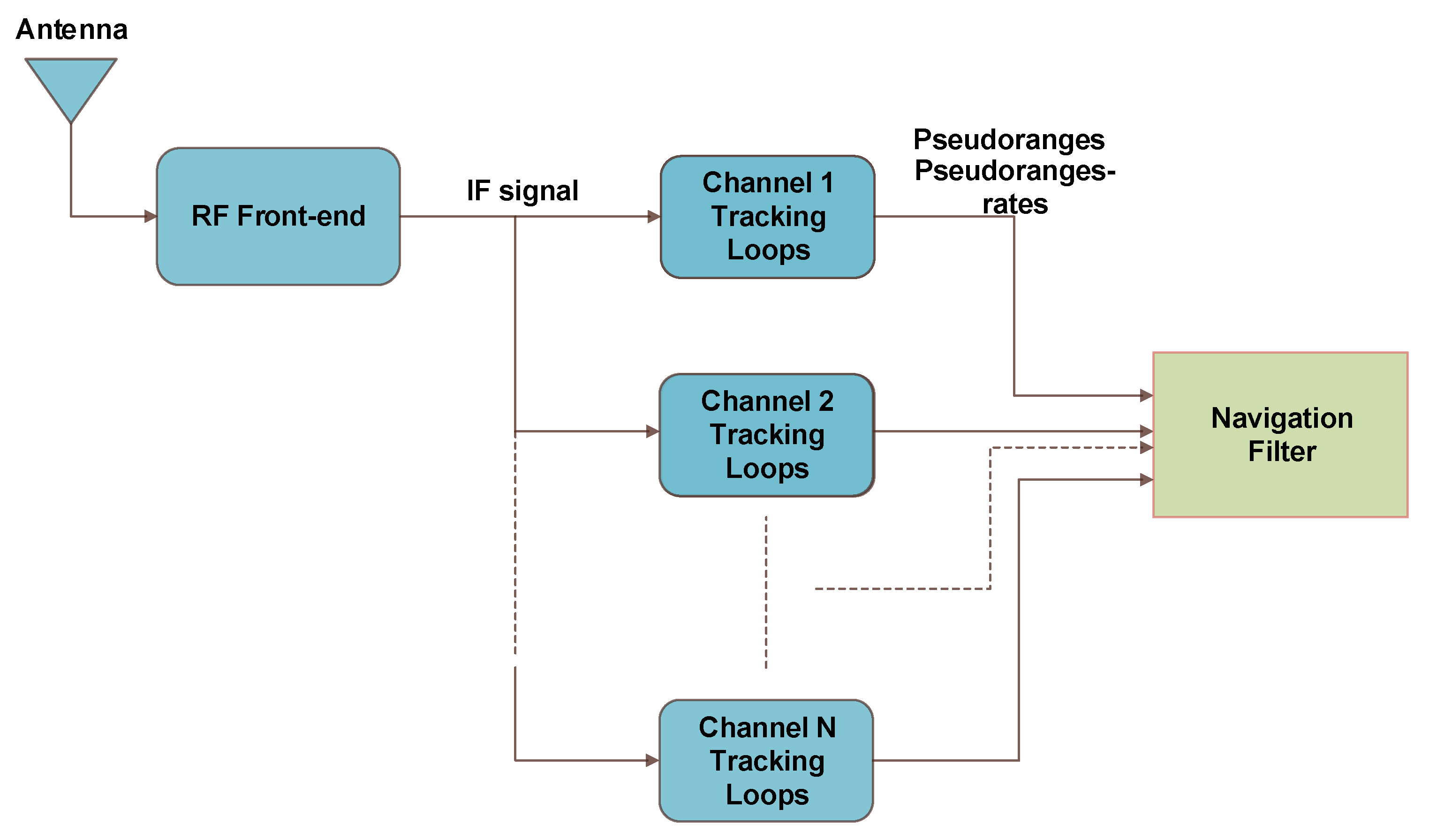Figure 1 shows a block diagram for a scalar system tracking N satellites. Pseudoranges and pseudorange rates are separately generated and only processed together in the navigation filter. Thus, no information exchange happens between the different tracking channels in this mechanism. Vector-based tracking, on the other hand, feeds back [7,8,9] any available information about receiver position, velocity, and acceleration to the tracking stage. In this way, information exchange between the different channels is possible, allowing improved performance in conditions where there is low signal power or poor satellite availability. 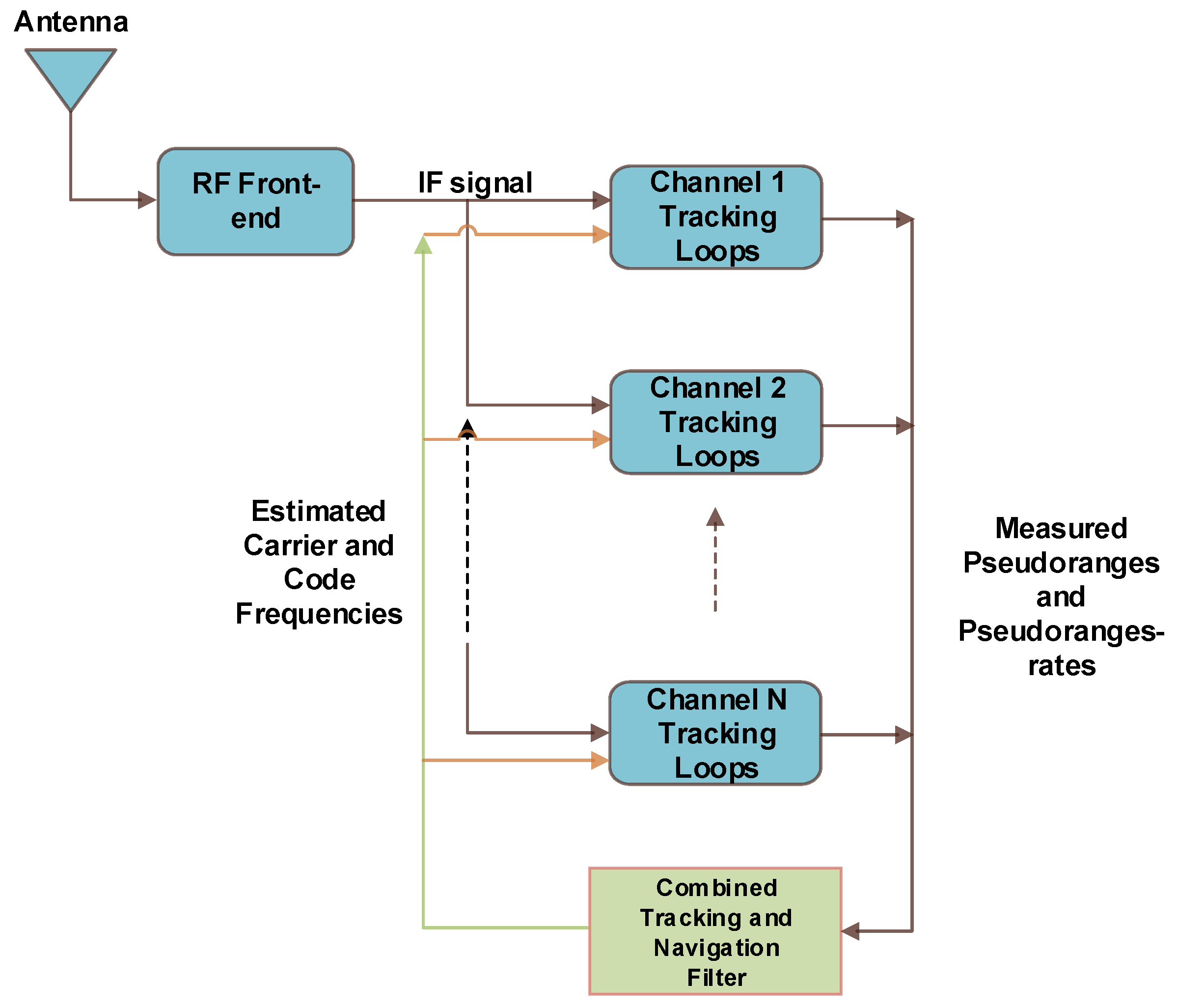Figure 2 gives an overview of the general architecture of vector tracking systems. Vector tracking systems combine all the channels to produce pseudoranges and pseudorange rates and the navigation solution in one filter. The early designs also use Costas tracking loops as their core blocks. State estimation algorithms have been effectively introduced into vector-based tracking systems. At the forefront of these algorithms is the Kalman filter, in a range of versions and configurations. Several implementations employing this filter in vector tracking showed improved performance over scalar tracking systems. Nonetheless, most of the related research recommends further investigation into more efficient algorithms with faster response and less complexity. Supporting vector-based tracking systems with information from external sources can further improve their performance and reliability. INS systems are a popular choice of such a supplementary source. However, augmenting a GPS with an INS that uses a full inertial measurement unit (IMU) comes with the penalty of higher complexity and increased cost. Thus, recent research has been directed towards the use of Micro-Electro-Mechanical Systems (MEMS) grade inertial sensors for low cost navigation applications [6]. Nonetheless, these inexpensive sensors have complex error characteristics; therefore, the latest research is conducted to utilize a smaller number of inertial sensors inside the IMU to obtain the navigation solution [10]. Advantage of this trend is twofold. The first is to avoid the effect of the inertial sensor errors. The second is to reduce the cost of the IMU in general [11]. One such approach known as RISS (Reduced Inertial Sensor System) is discussed in [10,11,12,13]. This paper investigates using RISS to provide an efficient, reliable, yet less complex and inexpensive ultra-tight GPS/INS integrated solution. Augmenting GPS vector-tracking loops with the RISS, the proposed ultra-tight GPS/INS integrated solution, as discussed below, uses specific models that are different from its counterparts reported in literature. Furthermore, the performance of the introduced system is also tested using a unique GPS/INS setup that has been implemented on the side of this work.

It is a fact that GPS is not the only operational GNSS anymore. Hence, multi-constellation and multi-frequency GNSS is one of the more realistic solutions to the problem discussed in this paper. However, there are number of applications that require relying on a single-constellation system. For example, for some strategic applications, there is an essential demand to explore solutions relying only on the GPS constellation and in most cases involving only one of the carrier frequencies. Some of the future civilian and rescue services applications require relying only on GPS and most of them either rely on L1 GPS or L5 GPS. This research addresses the issue of aiding single constellation (GPS) operating at one carrier frequency with other self-contained navigation systems, i.e., INS, rather than using multi-constellations. However, the concepts introduced in this paper can similarly be applied to other satellite-based navigation systems.

Different forms of ultra-tightly coupled GPS/INS integration systems have been presented in literature using either different integration algorithms and/or sensors configuration. A Kalman filter-based design is proposed in [14] that combines the GPS and INS systems at the correlator output stage of the GPS receiver with the conventional code/carrier tracking loops merged in the integration Kalman filter. Research in [15] proposed a GPS/INS integrated based on what is called multi-channel cooperated tracking (COOP tracking). The INS and COOP loops operate together to provide a nearly perfect reference for receiver dynamics and receiver clock errors. Thus, the PLL/DLL loops track the differences between the incoming and the local signals, which have been compensated by INS and COOP loops. In [16] researchers propose a strategy of an ultra-tight GPS/INS integration system based on an unscented Kalman filter (UKF). The GPS/INS ultra-tight integration system exploit the position velocity and attitude which are obtained from INS to estimate the I/Q signal, then the I/Q error formed by INS estimation and GPS measurement can be obtained. Research in [10] introduced an ultra-tight integration system to fuse GPS and reduced IMU configuration consisting of two horizontal accelerometers, a single vertical gyroscope, and wheel speed sensors. The paper investigates the feasibility of the proposed method for the ultra-tight integration for land vehicle navigation applications. Research in [17] is extension of what is proposed in [10]. A major addition was the use of dual frequency receiver to overcome some limitations experienced by the legacy L1 C/A signals. A combination of L1 and L2C signals, available in modern receivers, was used to obtain improved observability and therefore better navigation performance. In [18], researchers applied an adaptive unscented Kalman filter which prudently selects deterministic sigma points from Gaussian distributions and propagates these points through a nonlinear function. Besides, the Scaled Unscented Transformation (SUT) method was selected for the sigma point selection, which gave the ability to alter the spread of sigma points and control the higher order errors through some design parameters. An improved ultra-tightly GPS/INS integration approach is proposed in [19]. The method makes use of the neural network (NN) to improve the quality of the Doppler estimates from the Kalman filter. The algorithm is meant for seamless navigation during GPS outages. Research in [20] presents a state estimation technique for pre-filter signal states estimate for the ultra-tight GPS/INS navigation. A fuzzy logic system is selected to improve the UKF performance and to prevent the filter divergence problem in the high dynamic environments and periods of the partial GPS outages. An unscented particle filter (UPF) is also added to the system as a pre-filtering technique to deal with the non-linear, non-Gaussian disturbances and leads to the significant accuracy improvement. A comprehensive comparison between tightly coupled integration and ultra-tight integration is given in [21]. The paper presents a fair analysis of tight coupling and deep integration as using same grade IMUs, satellite constellations, and GPS signal processing techniques. Authors in [22] presented an overview of various methods used to mitigate the impact on GNSS receivers caused by both unintentional and intentional jamming. The paper concluded that all the methods are helpful for jamming mitigation when applied individually but, also two or more methods can be integrated in one system. Authors in [23] proposed a method for tracking dual-frequency BeiDou B1/B2 signals simultaneously in a vector tracking architecture to construct an ultra-tightly coupled GNSS/INS system. The article reported that the proposed method can considerably enhance the tracking and navigation performance with respect to scalar tracking systems, but without showing any details about the type/characteristics of the used jamming signals.

The main objective of this paper is to introduce an efficient ultra-tight GPS/3D Reduced Inertial Sensor System (RISS) integrated system that enhances the GPS receiver tracking robustness and sensitivity in challenging scenarios and, consequently, improves navigation availability.

2. Ultra-Tight GPS/INS Integration and RISS

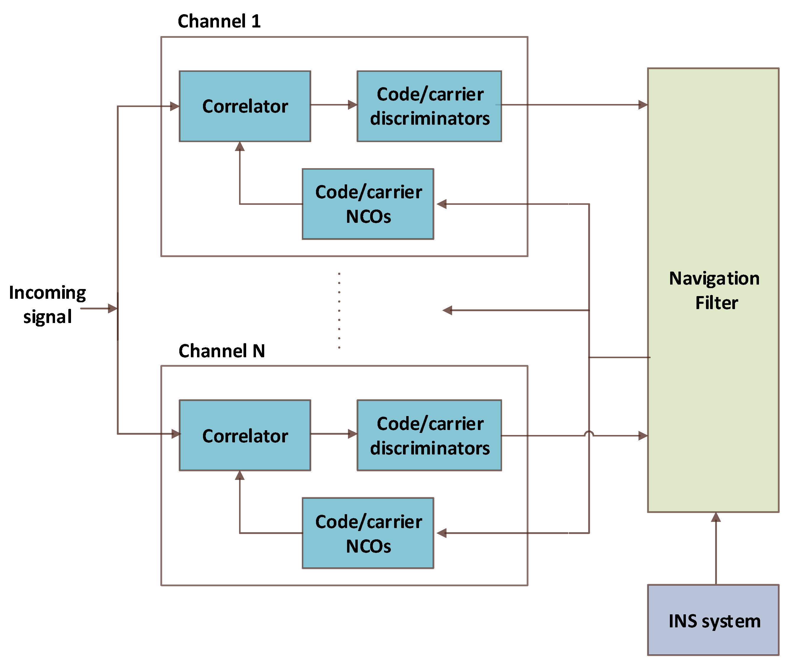
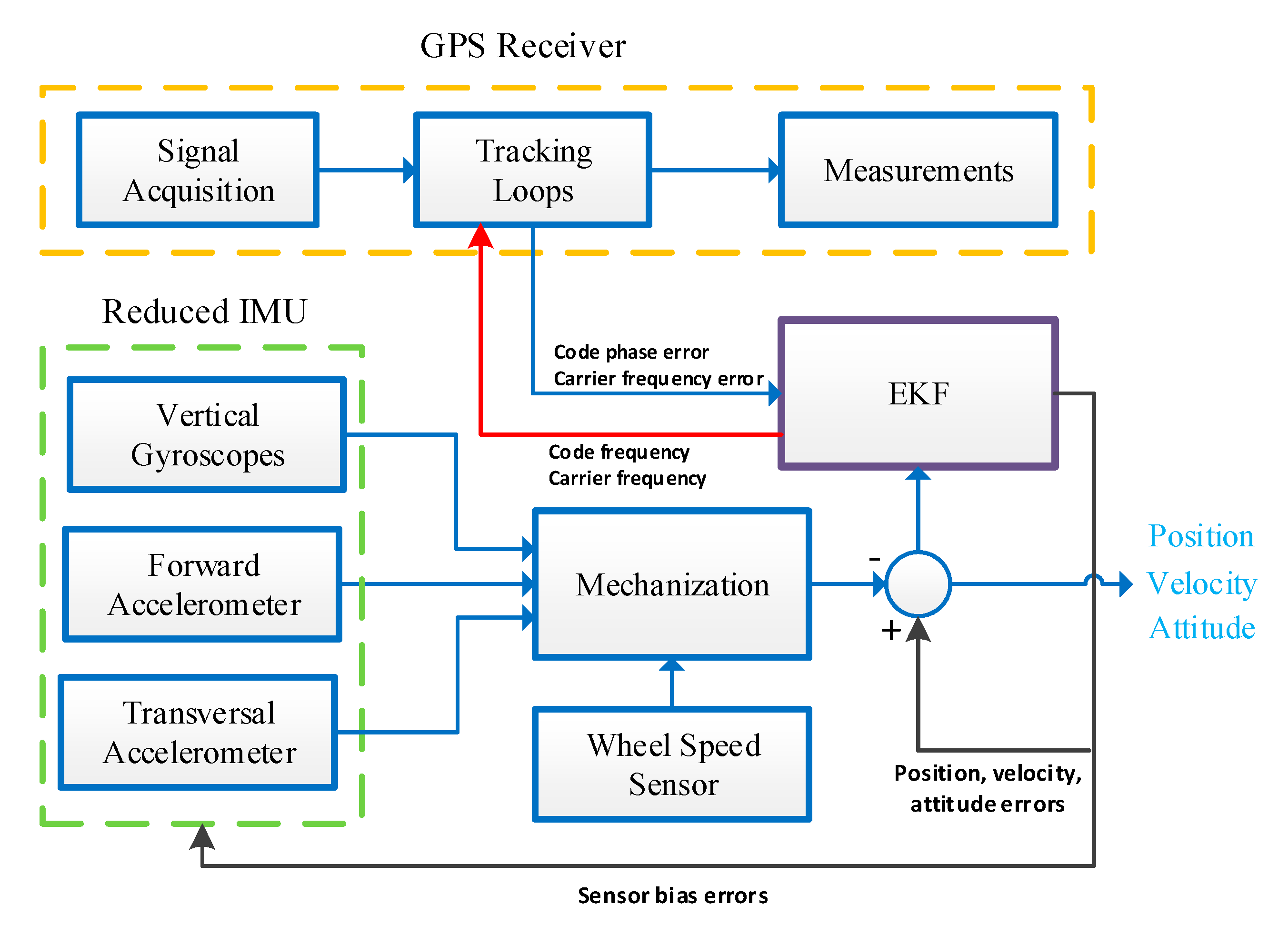
The ultra-tightly coupled integration, which is the state-of-the-art for GPS/INS integration, has been investigated over the past two decades. In this approach, as can be seen in Figure 3, the GPS raw measurements come directly from the front end of the GPS receiver, in the form of In-phase (I) and quadrature (Q) signal samples [24,25]. The correlator outputs I and Q are fed into the integration filter as measurements. Thus, estimated Doppler can be used to assist the tracking loops during GPS signal outages or under high receiver dynamics [26,27]. The integration of INS derived Doppler feedback to the carrier tracking loops provides a vital benefit to this system; the INS Doppler aiding removes the vehicle Doppler from the GPS signal; hence, it results in a major reduction in the carrier tracking loop bandwidth [22]. The bandwidth reduction, in turn, improves the anti-jamming performance of the receiver and, hence, increases the post correlated signal strength. In addition, due to lower bandwidths, the accuracy of the raw measurements is likewise increased [19].

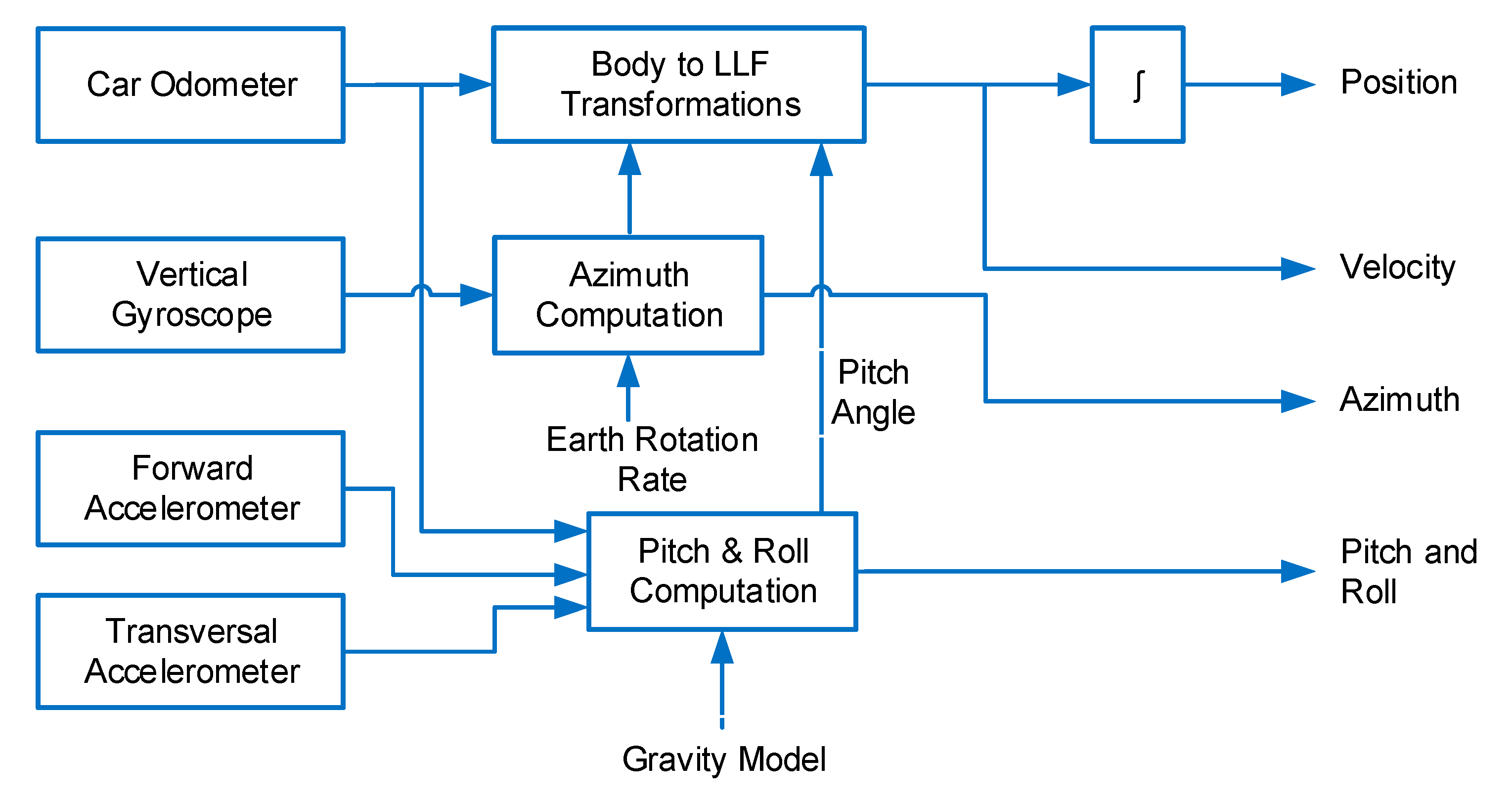
It was briefly mentioned above that the proposed method uses a 3D Reduced Inertial Sensor System (RISS) to develop a low-cost, simple, and efficient ultra-tightly coupled GPS/INS integrated system. Details about the origins of the adopted RISS system can be found in [11,12,13]. The RISS system uses measurements from one gyroscope, two accelerometers, and the built-in car odometer to generate a 3D navigational solution. The gyroscope is aligned with the vertical axes of the vehicle frame; while, the two accelerometers are mounted to the forward and transversal directions, respectively. This simple configuration is popular due to the fact that it provides superior performance over traditional 3D IMU systems at a lower cost [28].

2.1. RISS Motion Equations

The 3D RISS navigation state vector consists of nine parameters as the following:

$$X={\left[\phi ,\lambda ,h,{\upsilon }_e,{\upsilon }_n,{\upsilon }_u,r,p,A\right]}^T$$

(1)

where $\phi ,\lambda$ and $h$ are the position components, latitude, longitude, and altitude, respectively. ${\upsilon }_e,{\upsilon }_n,$ and ${\upsilon }_u$ are the velocity components, east velocity, north velocity, and up velocity, respectively. $r, p,$ and $A$ are the attitude components, roll, pitch, and azimuth, respectively. The calculations of the navigation solution are given in the next subsections. It should be mentioned here that the axes of the accelerometers and gyroscopes are set to match with the axes of the moving vehicle (the car in this application). Thus, a transformation operation is applied to obtain the navigation parameters with respect to a local-level frame (LLF) which represents the vehicle’s attitude and velocity information on or near the Earth’s surface.

2.2. Attitude Equations

First step is the azimuth angle calculation, which is obtained by removing the rotational components due to the transport rate and Earth rotation rate and then the integration of the gyroscope measurement. An assumption is set in land vehicle applications that vehicles are most of the time travelling in the horizontal plane. Hence, we can assume relatively small pitch and roll angles. Thus, the rate of change of the azimuth angle can be written as:

$$\dot{A}\approx -\left[\left({\omega }_z-b_z\right)-{\omega }^e\sin \phi -\frac{{\upsilon }_e\tan \phi }{R_N+h}\right]$$

(2)

where $\dot{A}$ is the rate of change of the azimuth angle, ${\omega }_z$ is gyroscope’s measurement, $b_z$ is the gyroscope bias, $\phi$ is latitude, ${\upsilon }_e$ is east velocity, ${\omega }^e$ is the Earth rotation rate, $h$ is the altitude of the vehicle and $R_N$ is the normal radius of the Earth’s ellipsoid.

Second, the pitch and roll angles are derived from accelerometer readings after compensating for accelerations due to forward speed and transversal acceleration component, respectively. The pitch angle is calculated as:

$$p={\sin }^{-1}\left(\frac{f_y-a_0}{g}\right)$$

(3)

where $f_y$ is the forward accelerometer measurement, $a_0$ is the vehicle acceleration derived from the vehicle odometer, and $g$ is the Earth’s gravity. The roll angle is calculated as:

$$r=-{\sin }^{-1}\left(\frac{f_x+{\upsilon }_o\left({\omega }_z-b_z\right)}{g\cos p}\right)$$

(4)

where $f_x$ is the transversal accelerometer measurement, ${\upsilon }_o$ is the vehicle speed obtained from the vehicle odometer.

2.3. Velocity Equations

After the azimuth and pitch angles are obtained, forward vehicle velocity can be projected into East, North, and Up velocities as the following:

$${\upsilon }_e={\upsilon }_o\sin A\cos p$$

(5)

$${\upsilon }_n={\upsilon }_o\cos A\cos p$$

(6)

$${\upsilon }_u={\upsilon }_o\sin p$$

(7)

2.4. Position Equations

Finally, the horizontal velocity components are converted into geodetic coordinates and then integrated to obtain a horizontal position in latitude and longitude form. The Up velocity is integrated to obtain altitude.

$$\dot{\phi }=\frac{{\upsilon }_n}{R_M+h}$$

(8)

$$\dot{\lambda }=\frac{{\upsilon }_e}{\left(R_N+h\right)\cos \phi }$$

(9)

$$\dot{h}={\upsilon }_u$$

(10)

where $R_M$ is the Meridian radius of the Earth’s ellipsoid. A high-level diagram of RISS mechanization is given in Figure 4.

3. The Proposed Method

The proposed ultra-tight GPS/INS integration system uses a centralized Kalman filter. The filter is updated from the tracking loops discriminators and its states are used to predict the pseudoranges and pseudorange-rates between measurement epochs. The estimates of the filter residuals (in accordance with the line of sight (LOS) geometry) are passed to correct the filter’s predicted pseudoranges and pseudorange-rates. The filter also applies its estimates of the IMU error states to correct the IMU data. In the ultra-tightly coupled GPS/INS integration, the signals from the receiver correlator, I and Q components, form the measurements of the filters. These I and Q measurements are integrated with the position, velocity and attitude of the INS. The code phase and Doppler shift calculated from the INS and satellite ephemeris are used to control both the code numerically controlled oscillator (NCO) and carrier NCO. The number of measurements is twice of the number of satellites being used for navigation.

In the ultra-tightly coupled GPS/INS integration, the measurement errors are obtained directly from the tracking loops not at the navigation filter level. In fact, the pseudorange errors and pseudorange rate errors are the scaled code phase errors and frequency errors, respectively. Every time a full cycle of tracking/navigation is completed, the carrier frequency and code frequency are estimated and fed back into the tracking loops. A high-level diagram of the proposed system is depicted in Figure 5.

3.1. GPS/3D RISS Integration

Looking into Equations (1) to (10) one can see that the major source of error in the RISS system is the gyroscope measurement error (mainly gyroscope bias) since it is inherent in the azimuth calculations which is further enlarged when integrated to calculate the horizontal velocity and then horizontal position components [12]. The accelerometers errors have a small effect since no integration is involved in the roll and pitch calculations equations. Thus, the roll and pitch angles are not included in the integrated solution.

3.1.1. The RISS System Model

To be integrated with GPS system models, the RISS equations need to be first linearized [11]. The Taylor series expansion method is used to achieve this linearization process. Then, the target error state vector of the 3D RISS becomes:

$$\delta X_{RISS}={\left[\delta \phi ,\delta \lambda ,\delta h,\delta {\upsilon }_e,\delta {\upsilon }_n,\delta {\upsilon }_u,\delta A,\delta a_o,\delta b_z\right]}^T$$

(11)

where $\delta \phi ,\delta \lambda ,$ and $\delta h$ are the errors in position components, latitude, longitude, and altitude, respectively. $\delta {\upsilon }_e,\delta {\upsilon }_n,$ and $\delta {\upsilon }_u$ are the errors in velocity components, east velocity, north velocity, and up velocity, respectively. $\delta A$ is the azimuth error, $\delta a_o$ is an error in acceleration derived from vehicle odometer, and $\delta b_z$ is the gyroscope bias error, respectively. Once again, the RISS motion equations in Section 2.3 are linearized using Taylor’s series expansion method so that we can get the rate of change of error states for the RISS system model. The derivations are well documented in the above-mentioned sources; therefore, we will give here the only final models which will be augmented in our proposed ultra-tightly GPS/RISS integrated system.

Attitude Errors Models

As mentioned above, the only attitude parameter included in the error state vector is the error in azimuth angle. The error in the azimuth rate of change is expressed as:

$$\delta \dot{A}\approx \underset{T_{12,1}}{\underbrace{1}}\times \delta b_z+\underset{T_{12,2}}{\underbrace{\left({\omega }^e\cos \phi +\frac{{\upsilon }_e{\sec }^2\phi }{R_N+h}\right)}}\delta \phi +\underset{T_{12,3}}{\underbrace{\frac{\tan \phi }{R_N+h}}}\delta {\upsilon }_e$$

(12)

Position Errors Models

After the linearization of Equations (9) and (10) with consideration of the error term in the azimuth rate of change, and omitting any negligible terms we get:

$$\delta \dot{\phi }\approx \underset{T_{13,1}}{\underbrace{\frac{1}{R_M+h}}} \delta {\upsilon }_n$$

(13)

$$\delta \dot{\lambda }\approx \underset{T_{14,1}}{\underbrace{\frac{1}{\left(R_N+h\right)\cos \phi }}}\delta {\upsilon }_e+\underset{T_{14,2}}{\underbrace{\frac{{\upsilon }_e\tan \phi }{\left(R_N+h\right)\cos \phi }}} \delta \phi$$

(14)

The rate of change of altitude is only related to the up velocity. After a simple linearization process, we get:

$$\delta \dot{h}=\underset{T_{15,1}}{\underbrace{\delta {\upsilon }_u}}$$

(15)

Velocity Errors Models

Likewise [6], linearizing Equations (5) and (6) for East and North velocities yields:

$$\begin{array}{c}\delta {\dot{\upsilon }}_e=\underset{T_{16,1}}{\underbrace{\sin A\cos p}} \delta a_o+\underset{T_{16,2}}{\underbrace{a_o\cos A\cos p}} \delta A-\underset{T_{16,3}}{\underbrace{({\omega }_z-b_z-{\omega }^e\sin \phi -\frac{{\upsilon }_e\tan \phi }{R_N+h})}}\delta {\upsilon }_n+\underset{T_{16,4}}{\underbrace{{\upsilon }_n}} \delta b_z\\ +\underset{T_{16,5}}{\underbrace{{\upsilon }_n({\omega }^e\cos \phi +\frac{{\upsilon }_e{\sec }^2\phi }{R_N+h})}}\delta \phi +\underset{T_{16,6}}{\underbrace{\frac{{\upsilon }_n\tan \phi }{R_N+h}}}\delta {\upsilon }_e\end{array}$$

(16)

$$\begin{array}{c}\delta {\dot{\upsilon }}_n=\underset{T_{17,1}}{\underbrace{\cos A\cos p}} \delta a_o-\underset{T_{17,2}}{\underbrace{a_o\sin A\cos p}} \delta A+\underset{T_{17,3}}{\underbrace{({\omega }_z-b_z-{\omega }^e\sin \phi -\frac{2{\upsilon }_e\tan \phi }{R_N+h})}}\delta {\upsilon }_e-\underset{T_{17,7}}{\underbrace{{\upsilon }_e}} \delta b_z\\ -\underset{T_{17,5}}{\underbrace{{\upsilon }_e({\omega }^e\cos \phi +\frac{{\upsilon }_e{\sec }^2\phi }{R_N+h})}}\delta \phi \end{array}$$

(17)

Up velocity is independent of azimuth errors, and hence, derivations are much simpler:

$$\delta {\dot{\upsilon }}_u=\underset{T_{18,1}}{\underbrace{\sin p}} \delta a_o$$

(18)

Vehicle Odometer Error Model

The odometer error is modeled as a first-order Gauss–Markov process [12]:

$$\delta {\dot{a}}_o=\underset{T_{19,1}}{\underbrace{-{\beta }_o}} \delta a_o+\sqrt{2{\beta }_o{\sigma }_o^2}w\left(t\right)$$

(19)

where ${\beta }_o$ is the reciprocal of the sensor data correlation time, ${\sigma }_o$ is the standard deviation of the error, and $w\left(t\right)$ is the noise term.

Gyroscope Error Model

Similarly, the gyroscope error is modeled using a first-order Gauss–Markov process:

$$\delta {\dot{b}}_z=\underset{T_{20,1}}{\underbrace{-{\beta }_z}} \delta b_z+\sqrt{2{\beta }_z{\sigma }_z^2}w\left(t\right)$$

(20)

where ${\beta }_z$ is the reciprocal of the sensor data correlation time, ${\sigma }_z$ is the standard deviation of the error, and $w\left(t\right)$ is the noise term.

3.1.2. The GPS System Model

Two states are normally added to model the GPS receiver clock errors which are the receiver clock bias $\delta b_r$ and the receiver clock drift $\delta d_r$. The GPS receiver clock drift is modelled first using a random walk process, and the receiver clock bias is integral of that.

$$\delta {\dot{b}}_r=\delta d_r$$

(21)

$$\delta {\dot{d}}_r={\sigma }_d{\omega }_G$$

(22)

where ${\omega }_G$ is white Gaussian noise and ${\sigma }_d$ is the standard deviation of clock drift white noise. Thus, the state vector for the added GPS error states becomes:

$$\delta X_{GPS}={\left[\delta r_b,\delta r_d\right]}^T$$

(23)

Combining the two-state vectors from the RISS side and the GPS side, we obtain the complete state vector for the GPS/RISS integrated system:

$$\delta X={\left[\delta \phi ,\delta \lambda ,\delta h,\delta {\upsilon }_e,\delta {\upsilon }_n,\delta {\upsilon }_u,\delta A,\delta a_o,\delta b_z,\delta r_b,\delta r_d\right]}^T$$

(24)

Now that we have all the error models; thus, we can form the system transition matrix as given in Equation (25). Writing the actual terms in the system transition matrix will make it look awkward; hence, we used some notation to write a compact version of that. Other than the zeros and ones, the terms in the matrix are on the form $T_{j,k}$ where $j$ is the equation number from which we obtain that term and $j$ is the order of the term in the same equation. For instance, $T_{16,4}$ means the fourth term in Equation (16) (or portion of that as underlined in the equation itself).

$$F=\left[\begin{array}{ccccccccccc}0& 0& 0& 0& T_{13,1}& 0& 0& 0& 0& 0& 0\\ T_{14,2}& 0& 0& T_{14,1}& 0& 0& 0& 0& 0& 0& 0\\ 0& 0& 0& 0& 0& 1& 0& 0& 0& 0& 0\\ T_{16,5}& 0& 0& T_{16,6}& T_{16,3}& 0& T_{16,2}& T_{16,1}& T_{16,4}& 0& 0\\ T_{17,5}& 0& 0& T_{17,3}& 0& 0& T_{17,2}& T_{17,1}& T_{17,4}& 0& 0\\ 0& 0& 0& 0& 0& 0& 0& T_{18,1}& 0& 0& 0\\ T_{12,2}& 0& 0& T_{12,3}& 0& 0& 0& 0& T_{12,1}& 0& 0\\ 0& 0& 0& 0& 0& 0& 0& T_{19,1}& 0& 0& 0\\ 0& 0& 0& 0& 0& 0& 0& 0& T_{20,1}& 0& 0\\ 0& 0& 0& 0& 0& 0& 0& 0& 0& 0& 1\\ 0& 0& 0& 0& 0& 0& 0& 0& 0& 0& 0\end{array}\right]$$

(25)

The complete state vector for the system can be expressed as:

$$\delta \dot{x}=F\delta x+Gw$$

(26)

where $\delta \dot{x}$ is the current (predicted) error state vector, $\delta x$ is the last error state vector, $G$ is the noise coupling matrix, and $w$ is the noise vector. The expanded form of this equation can be written as follows:

$$\left[\begin{array}{c}\delta \dot{\phi }\\ \delta \dot{\lambda }\\ \delta \dot{h}\\ \delta {\dot{\upsilon }}_e\\ \delta {\dot{\upsilon }}_n\\ \delta {\dot{\upsilon }}_u\\ \delta \dot{A}\\ \delta {\dot{a}}_o\\ \delta {\dot{b}}_z\\ \delta {\dot{r}}_b\\ \delta {\dot{r}}_d\end{array}\right]=[F]\left[\begin{array}{c}\delta \phi \\ \delta \lambda \\ \delta h\\ \delta {\upsilon }_e\\ \delta {\upsilon }_n\\ \delta {\upsilon }_u\\ \delta A\\ \delta a_o\\ \delta b_z\\ \delta r_b\\ \delta r_d\end{array}\right]+\left[\begin{array}{c}0\\ 0\\ 0\\ 0\\ 0\\ 0\\ 0\\ \sqrt{2{\beta }_o{\sigma }_o^2}\\ \sqrt{2{\beta }_z{\sigma }_z^2}\\ 0\\ 0\end{array}\right]w$$

(27)

3.1.3. The System Measurement Model

The GPS-only system uses an Earth-centered Earth-fixed (ECEF) frame of reference as the state vector reflects whereas the complete (integrated) system state vector is in Local Level Frame (LLF). Thus, we need to project this into that then we can connect the measurements with the system states for the system measurement update step. The errors in the pseudorange measurements are connected to the errors in the position through the following relation [6]:

$$\delta Z_p=\left[\begin{array}{c}\delta {\rho }^1\\ ⋮\\ \delta {\rho }^N\end{array}\right]=\left[\begin{array}{ccc}{L}_x^1& L_y^1& L_z^1\\ L_x^2& L_y^2& L_z^2\\ ⋮& ⋮& ⋮\\ L_x^N& L_y^N& L_z^N\end{array}\right]\left[\begin{array}{c}\delta x\\ \delta y\\ \delta z\end{array}\right]+\delta b_r+\left[\begin{array}{c}{\epsilon }_p^1\\ ⋮\\ {\epsilon }_p^N\end{array}\right]$$

(28)

$$\delta {\rho }^j={\rho }_{GPS}^j-{\rho }_{est}^j$$

(29)

where ${\rho }_{GPS}^j$ is the pseudorange measured by the GPS receiver to the jth satellite, ${\rho }_{est}^j$ is the estimated pseudorange to the jth satellite, ($L_x^j, L_y^j, L_z^j)$ is the line-of-sight vector from receiver to the jth satellite, ${\left[{\epsilon }_p\right]}_{N\times 1}$ is the pseudorange measurement noise vector.

The transformation matrix above, also called the geometry matrix, will henceforth be denoted as $G$.

We use the following relation to transform the ECEF Cartesian coordinates into ECEF geodetic coordinates:

$$x=\left(R_N+h\right)\cos \phi \cos \lambda$$

(30)

$$y=\left(R_N+h\right)\cos \phi \sin \lambda$$

(31)

$$z=\left[R_N\left(1-e^2\right)+h\right]\sin \phi$$

(32)

However, since we are interested in the error terms of these coordinates, again we linearize this relation and then get:

$$\left[\begin{array}{c}\delta x\\ \delta y\\ \delta z\end{array}\right]=\left[\begin{array}{ccc}-\left(R_N+h\right)\sin \phi \cos \lambda & -\left(R_N+h\right)\cos \phi \sin \lambda & \cos \phi \cos \lambda \\ -\left(R_N+h\right)\sin \phi \sin \lambda & +\left(R_N+h\right)\cos \phi \cos \lambda & \cos \phi \sin \lambda \\ \left[R_N\left(1-e^2\right)+h\right]\cos \phi & 0& \sin \phi \end{array}\right]\left[\begin{array}{c}\delta \phi \\ \delta \phi \\ \delta h\end{array}\right]$$

(33)

For simplicity, we will re-write the above equation on the form:

$$\delta r^e=T\delta r^l$$

(34)

where $\delta r^e$ represents the Cartesian position error vector, T is the transformation matrix, and $\delta r^l$ is the geodetic position error vector. Substituting Equation (34) into Equation (28), we get:

$$\delta Z_p=GT\delta r^l+\delta b_r+{\epsilon }_p$$

(35)

We will join the G and T matrices in one whole matrix for better readability:

$$H_{N\times 3}^p=G_{N\times 3}{T}_{3\times 3}$$

(36)

Thus, the ultimate pseudorange measurement model becomes:

$$\delta Z_{pN\times 1}=H_{N\times 3}^p\delta r^l+\delta b_r+{\epsilon }_{pN\times 1}$$

(37)

We deal with the pseudorange rate measurements in a similar way. The errors in the pseudorange rate measurements can be connected to the errors in velocity as:

$$\delta Z_{\dot{p}}=\left[\begin{array}{c}\delta {\dot{\rho }}^1\\ ⋮\\ \delta {\dot{\rho }}^N\end{array}\right]=\left[\begin{array}{ccc}{L}_x^1& L_y^1& L_z^1\\ L_x^2& L_y^2& L_z^2\\ ⋮& ⋮& ⋮\\ L_x^N& L_y^N& L_z^N\end{array}\right]\left[\begin{array}{c}\delta {\upsilon }_x\\ \delta {\upsilon }_y\\ \delta {\upsilon }_z\end{array}\right]+\delta d_r+\left[\begin{array}{c}{\epsilon }_{\dot{p}}^1\\ ⋮\\ {\epsilon }_{\dot{p}}^N\end{array}\right]$$

(38)

$$\delta {\dot{\rho }}^j={\dot{\rho }}_{GPS}^j-{\dot{\rho }}_{est}^j$$

(39)

where ${\dot{\rho }}_{GPS}^j$ is the pseudorange rate measured by the GPS receiver to the jth satellite, ${\dot{\rho }}_{est}^j$ is the estimated pseudorange rate to the jth satellite, ${\left[{\epsilon }_{\dot{p}}\right]}_{N\times 1}$ is the pseudorange rate measurement noise vector. The velocity error vector will be annotated as $\delta {\upsilon }^e$, and hence, Equation (36) becomes:

$$\delta Z_{\dot{p}}=G\delta {\upsilon }^e+\delta d_r+{\epsilon }_{\dot{p}}$$

(40)

The LLF-calculated velocity can be transformed into Earth Centred Earth Fixed velocity using:

$$\left[\begin{array}{c}\delta {\upsilon }_x\\ \delta {\upsilon }_y\\ \delta {\upsilon }_z\end{array}\right]=\left[\begin{array}{ccc}-\sin \lambda & -\sin \phi cos\lambda & \cos \phi \cos \lambda \\ \cos \lambda & -\sin \phi sin\lambda & \cos \phi \sin \lambda \\ 0& \cos \phi & \sin \phi \end{array}\right]\left[\begin{array}{c}\delta {\upsilon }_e\\ \delta {\upsilon }_n\\ \delta {\upsilon }_u\end{array}\right]$$

(41)

This LLF to ECEF transformation matrix will be denoted as $R_l^e$. Furthermore, the velocity error vector in the LLF will be denoted as $\delta {\upsilon }^l$. Therefore, the last equation becomes:

$$\delta {\upsilon }^e=R_l^e\delta {\upsilon }^l$$

(42)

Substituting this into Equation (40) we obtain:

$$\delta Z_{\dot{p}}=G{R}_l^e\delta {\upsilon }^l+\delta d_r+{\epsilon }_{\dot{p}}$$

(43)

We will combine the geometry matrix $G$ and the transformation matrix $R_l^e$ into one matrix:

$$H_{N\times 3}^{\dot{p}}=G_{N\times 3}{R}_{l3\times 3}^e$$

(44)

Thus, the final pseudorange rate measurement model could be expressed as:

$$\delta Z_{\dot{p}N\times 1}=H_{N\times 3}^{\dot{p}}\delta {\upsilon }^l+\delta d_r+{\epsilon }_{\dot{p}N\times 1}$$

(45)

Now the complete system measurement model could be formed by combining the pseudorange errors measurement model as in Equation (37) and pseudorange rate measurement errors as in Equation (45):

$$\delta Z_{2N\times 1}=H_{2N\times 11}\delta x_{11\times 1}+\left[\begin{array}{c}\delta b_{rN\times 1}\\ \delta d_{rN\times 1}\end{array}\right]+\left[\begin{array}{c}{\epsilon }_{pN\times 1}\\ {\epsilon }_{\dot{p}N\times 1}\end{array}\right]$$

(46)

where

$$H_{2N\times 11}=\left[\begin{array}{ccccc}{H}_{N\times 3}^p& 0_{N\times 3}& 0_{N\times 3}& 1_{N\times 1}& 0_{N\times 1}\\ 0_{N\times 3}& H_{N\times 3}^{\dot{p}}& 0_{N\times 3}& 0_{N\times 1}& 1_{N\times 1}\end{array}\right]$$

(47)

As discussed in Section 3, the pseudorange errors and pseudorange rate errors are the scaled code phase errors and frequency errors, as generated by the code and carrier frequency discriminators, respectively. These error terms can be expressed as:

$$\delta {\rho }_k^j=\frac{c\Delta {\tau }_k^j}{f_{code}}$$

(48)

$$\delta {\dot{\rho }}_k^j=\frac{c\Delta f_k^j}{f_{carrier}}$$

(49)

where c is the speed of light, $\mathsf{\Delta }\tau$ is the code phase error, $f_{code}$ is the code frequency = $1.023\times {10}^6\mathrm{Hz}$, $\mathsf{\Delta }f$ is the carrier frequency error, $f_{carrier}$ is the nominal L1 frequency = 1575.42 MHz, k represents the epoch number, and j is the corresponding satellite number.

Every time a cycle of the tracking/navigation process is completed, the carrier frequency and code frequency are estimated and fed back into the tracking loops to control the code and carrier NCOs inputs to align the locally generated signal with the incoming signal.

4. Experiment Work

This research used both simulation and real signal data to help in the design and validation of proposed method. Figure 6 illustrates experiment setup used in this research. For the GPS data, the GSS6700 Satellite Navigation Simulation Signal Generator, by Spirent, was used to design and generate the desired trajectory. The most important feature of the GSS6700 system is the repeatability function that enables it to provide wide dynamic capacity in GPS signal characteristics such as Doppler and signal power levels as well as enough channels to support in-view and multipath environments. To benefit from the trajectory scenarios generated by this system, it needs to be connected to a Front End (FE) unit. This research used the FireHose D17088, by NovAtel, as the front end unit to generate the in-phase (I), and quadrature-phase (Q) signals out of the data stream obtained from either the above-mentioned simulator or real trajectory data by connecting the unit to an antenna.

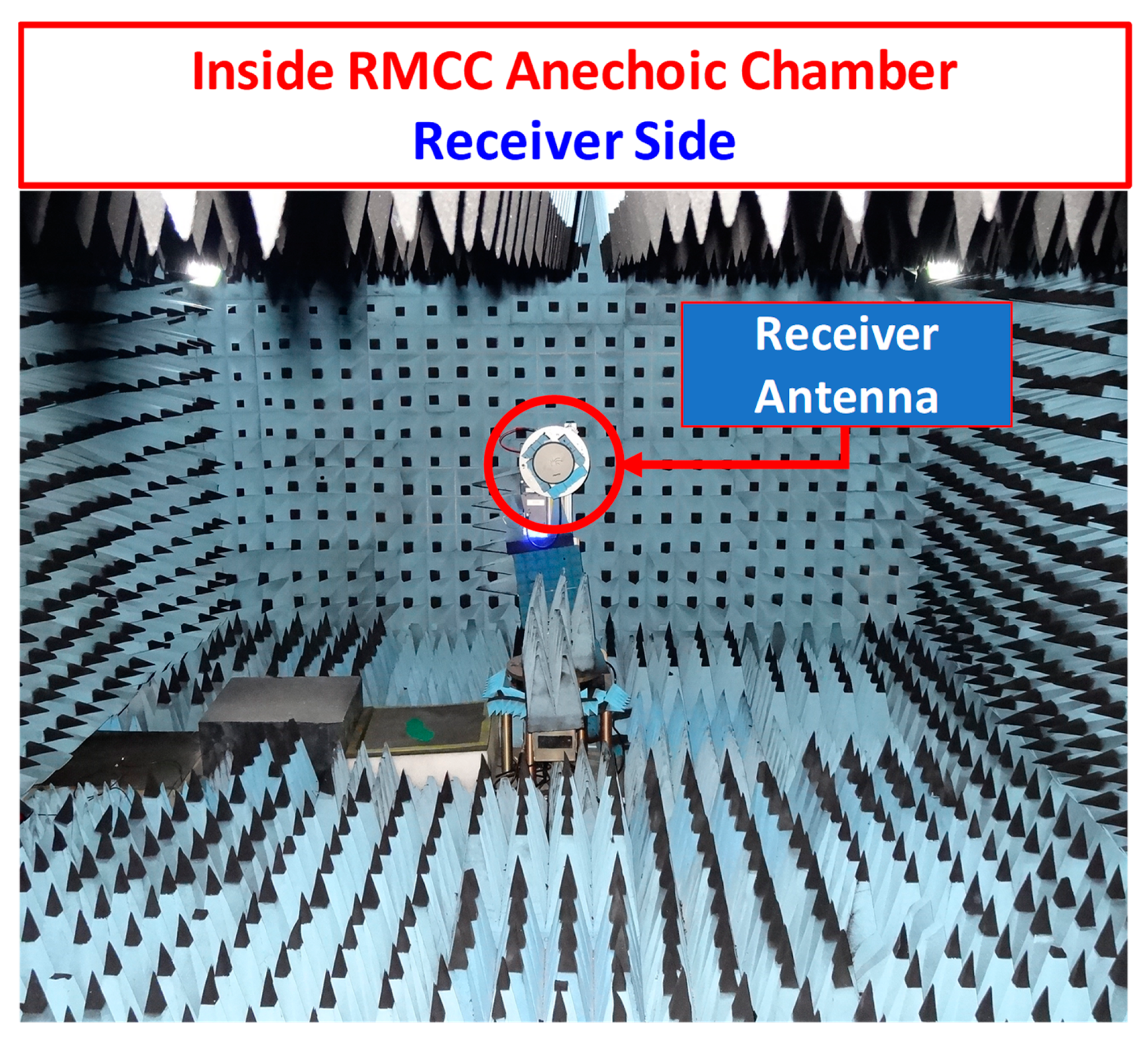
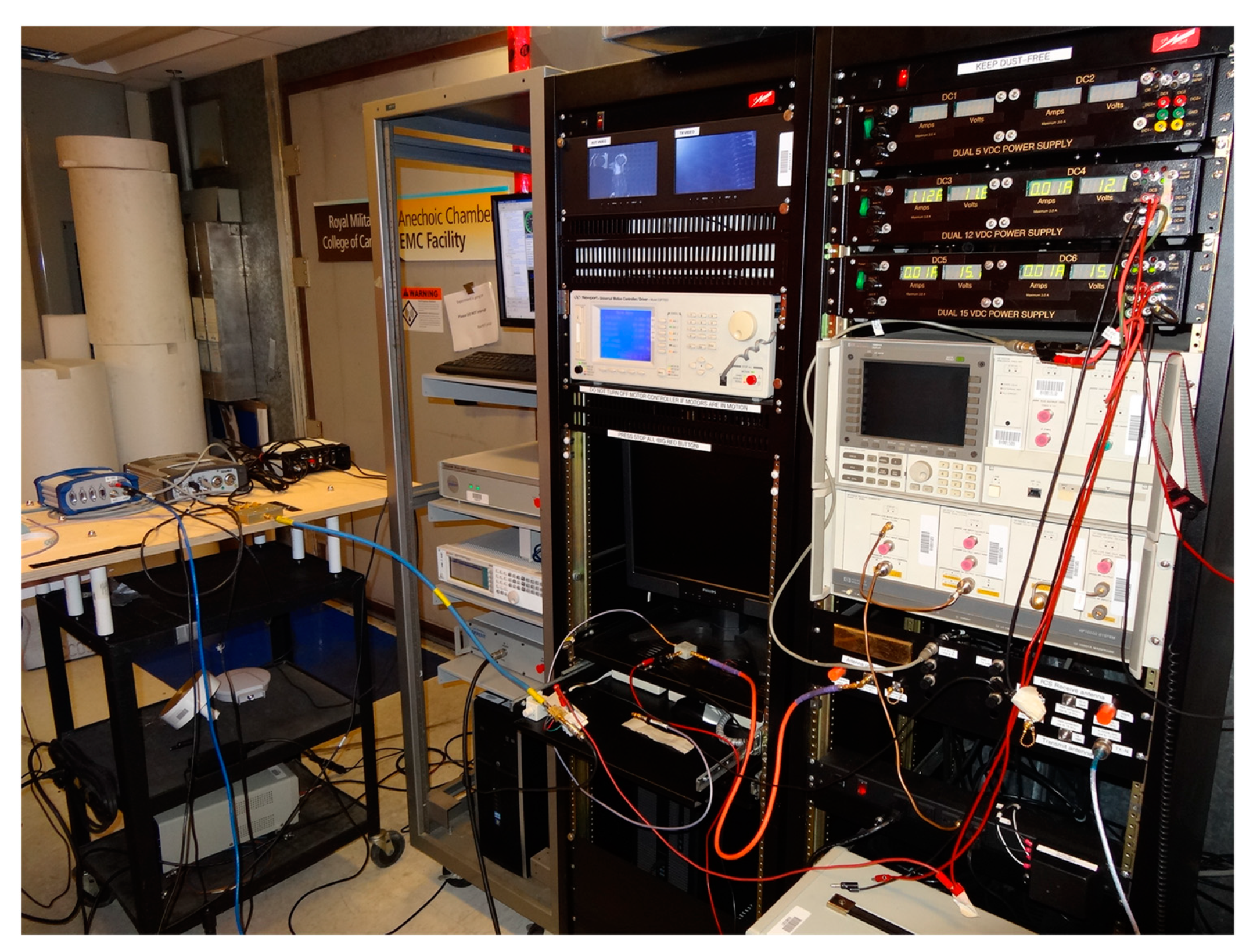
This research also comprises real GPS signal jamming experiments. This obviously requires the re-broadcast of the GPS signal to expose it to the real jammer signal. Thus, an exclusive and very interesting setup was built for this purpose. The real jamming signal experiments took place inside the Anechoic Chamber room at the Royal Military College of Canada (RMC). The room is designed with impenetrable walls and doors blocking any signals from entering or exiting the room. This guaranteed that the re-broadcast GPS signals and the real jammer signals could not penetrate to outside the room. The complete real jamming experiment setup is shown in Figure 7.

Note the use of a power amplifier at the transmitter side instead of a low noise amplifier (LNA) since the GPS signal power is normally below the noise floor. On the contrary, an LNA is used at the receiver side which will significantly amplify the received low-power GPS signal while keeping the noise induced by its circuitry minimum. Real pictures of the transmitter and receiver antenna inside the room are shown in Figure 8 and Figure 9, respectively. A picture of most of the devices used outside of the room is shown in Figure 10. The NovAtel NEAT jammer can work in high power and low power modes. Only low power mode has been used in this research. Furthermore, the device can generate four types of jamming signals: Narrow Band (NB), Wide Band (WB), Chirp, and Continues Wave (CW). The CW jamming type is chosen for the experiment shown in this work.

For the INS data sets, the INS Simulator, developed by the Mobile Multi-sensor Group at the University of Calgary, is used for simulating inertial measurement unit (IMU) raw data. This simulator can virtually generate the raw data measurements of any grade of IMUs such as navigation, tactical, and consumer-grade systems. While the simulator can generate raw IMU measurements using user-defined vehicle motion and dynamics, it can also accept externally injected vehicle dynamics from real trajectory data. The latter approach is used in this research.

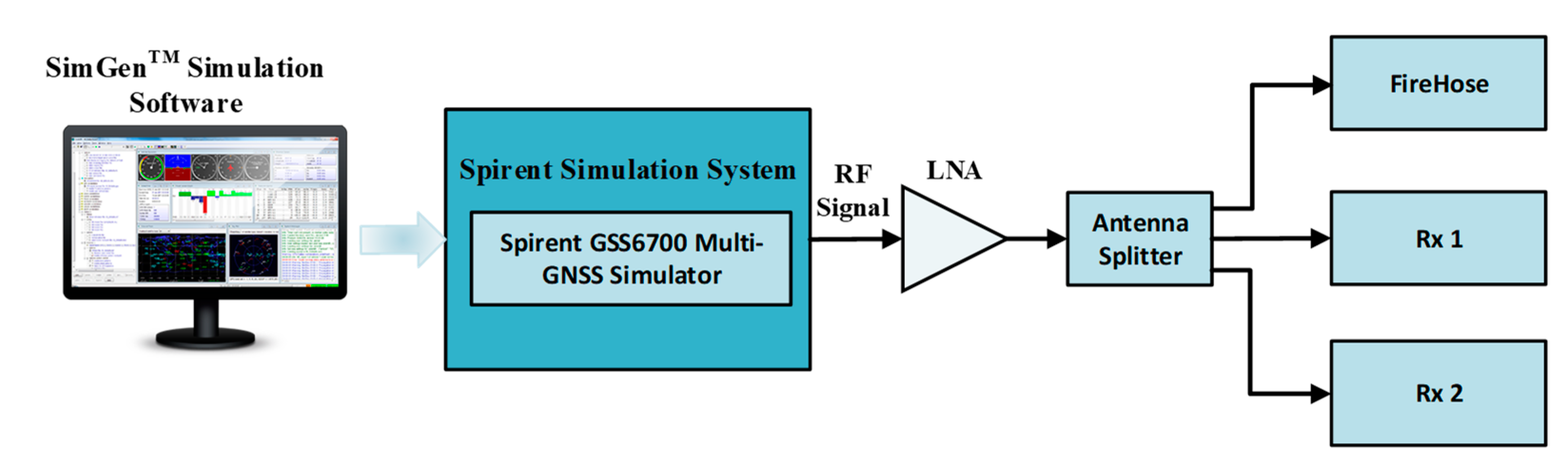
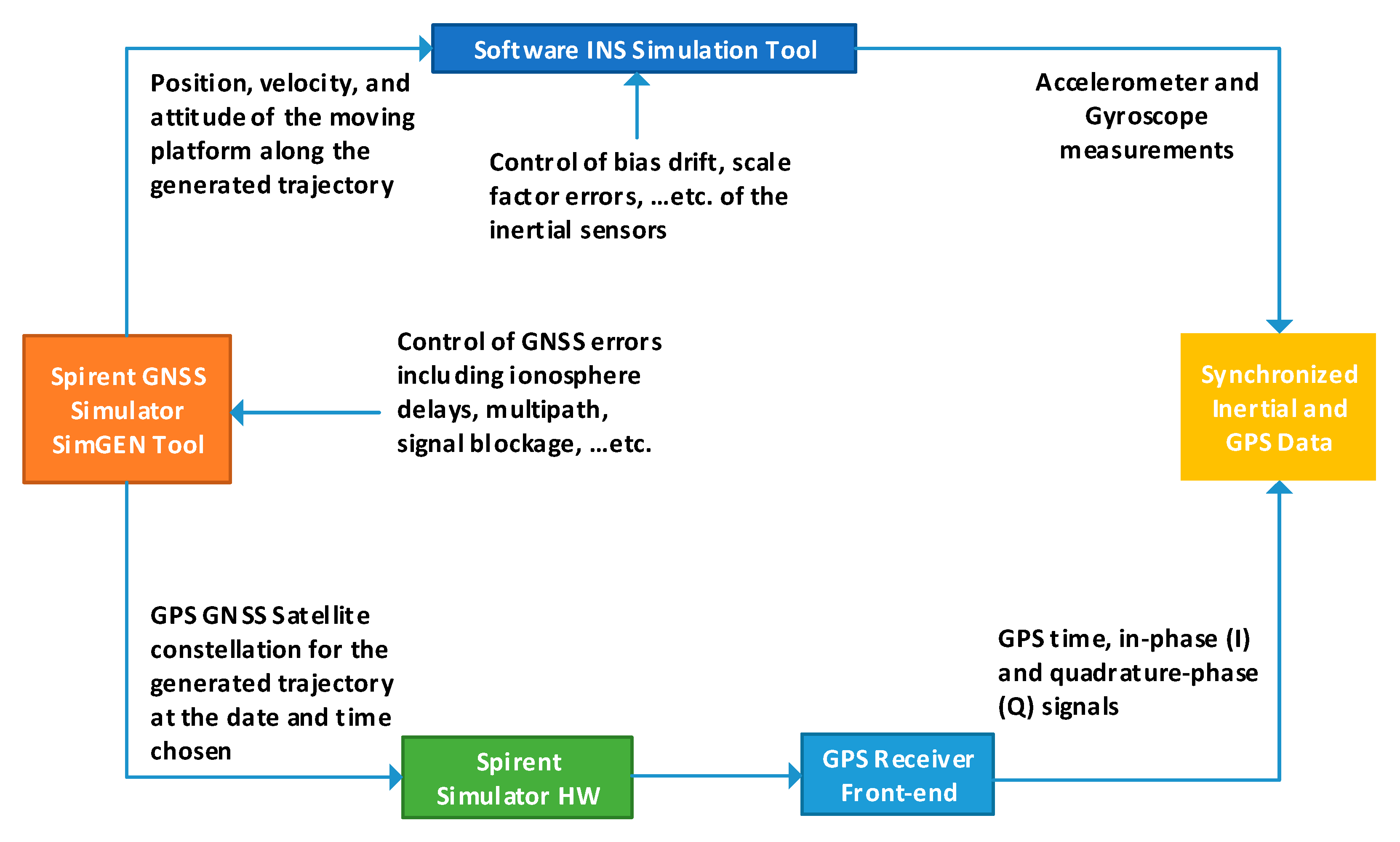
Figure 11 shows a high-level diagram of the trajectory data flow from the two arms of the complete signal/data simulation system used for both GPS and INS systems. The simulation process happens in three main steps. Step one-trajectory design when the general aspects of the trajectory such as the type of platform to be simulated, the satellite constellation, and the trajectory environment, are outlined. All of this is done using the Spirent SimGEN^TM software. Step two incorporates the implementation of the selected scenario and generating the data stream that is fed into the signal generator hardware (Spirents GSS6700), which in turn transforms this into a Radio Frequency (RF) signal. At the same time, the reference trajectory data are logged on the same computer that hosts the SimGEN^TM simulation software. Additionally, the I and Q branches are recorded, concurrently with the reference trajectory, on a GNSS receiver front-end, the FireHose by NovAtel.

Finally, the inertial data are simulated in step number three. First, the INS simulator is configured according to the desired simulation parameters such as the sensor data rate, grade of the selected sensor(s), and some initialization quantities that are obtained from the output of the GNSS signal simulator.

5. Results and Analysis

The selected trajectory is a simulation of a land vehicle driving at a constant speed of 36 km/h. The total trajectory length is 15 min. However, data logging started at five minutes into the trajectory time. The first few minutes are skipped to let the logging equipment ease into a steady state while receiving signals from the simulation hardware. Thus, the last ten minutes of the trajectory data are processed. Nevertheless, only about nine-and-a-half minutes are shown in the figures since the focus here is on the tracking and navigation stages where the first 36 s are used to extract the navigation message before the receiver can generate a position solution.

The odometer data rate was set to 100 Hz with a correlation time of one hour for the scale factor (SF) error. The odometer white noise standard deviation is 0.01 m/s. settings for the inertial sensors’ errors are given in

Table 1. IMU sensors specifications.

Gyroscope	Bias instability < 10 [deg/h]	Noise (ARW) 1 (deg/sqrt(hr))
Accelerometers	Bias instability 1 [deg/h]	Noise (VRW) 0.05 (m/s/sqrt(hr))

.

GPS signal jamming is one of the most critical error sources affecting navigation solutions across the world. Moreover, recent research demonstrates that GNSS/INS integration is now more important than ever due to the known immunity of INS against most of GNSS error sources including signal interference and jamming. Thus, it is important to examine the performance of the proposed method under jamming conditions. A low-power Continuous Wave (CW) jamming signal is selected. In this scenario, a real jamming signal is broadcast inside the anechoic chamber room. The spectrum of this signal is shown in Figure 12. This was obtained in the lab using a spectrum analyzer. From in lab analysis, and compared to a reference signal, it was found that the low power signal is about one Microwatt and the high-power signal is about one Milliwatt, millions of times stronger than a typical GPS signal. As can be seen Figure 12, the central frequency is around 1.5754 GHz, which is at the central frequency of the GPS system. A CW signal should theoretically have no bandwidth but since the system is nonideal, it is showing a bandwidth of 2.4 kHz. The jammer was turned on for 90 s, commencing at about three minutes from the beginning of the trajectory.

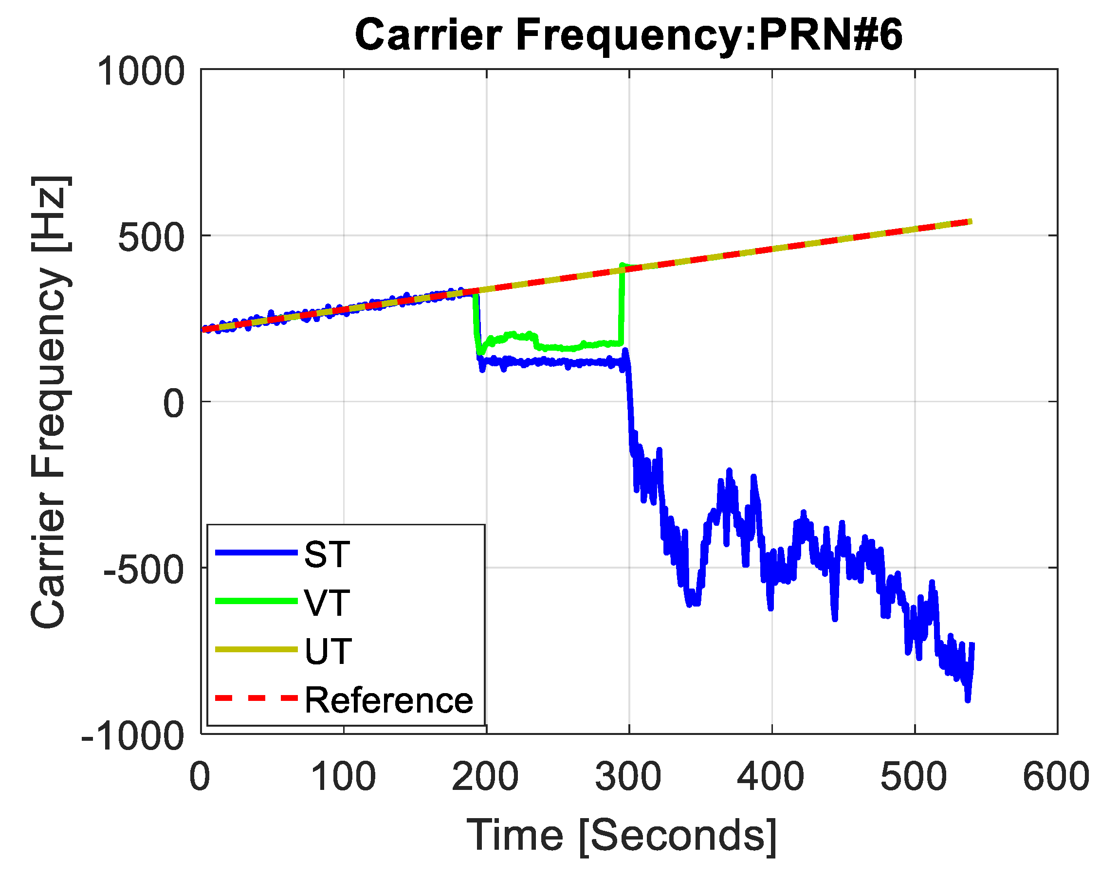
To make the discussion more valid, we here compare the performance of the introduced system versus a scalar tracking system (ST) and vector tracking system (VT), also implemented on the side of this work. Since the jamming signal frequency was around the GPS central frequency, most of the satellites in view were affected. Carrier frequencies of two sample satellites are shown in Figure 13 and Figure 14, respectively. The ST consequently lost track of some of the satellites leading to large position and velocity errors. The VT system was affected only when the jammer was on, but it immediately recovered tracking of all satellites signals once the jammer was off. This can be seen in the last two figures. The UT system experienced small errors and maintained the ability to track satellites signal even during the jamming period. The position and velocity error results for the three systems are summarized in

Table 2. Summary of position and velocity results.

RMS Errors
	ST	VT	UT
Ve (m/s)	105.09	18.64	0.0453
Vn (m/s)	104.00	3.55	0.6024
Vu (m/s)	96.42	4.94	0.0004
Spd2D (m/s)	147.85	18.97	0.6041
Spd3D (m/s)	176.52	19.61	0.6041
East (m)	110,762.21	150.48	5.5416
North (m)	270,450.61	19.86	17.42
Up (m)	1,266,843.69	17.53	3.8763
Pos2D (m)	292,252.97	151.79	18.28
Pos3D (m)	1,300,117.20	152.80	18.68
MAX Errors
	ST	VT	UT
Ve (m/s)	277.60	51.82	0.1860
Vn (m/s)	277.21	12.28	1.91
Vu (m/s)	198.15	30.01	0.0055
Spd2D (m/s)	392.31	53.25	1.92
Spd3D (m/s)	439.51	61.13	1.92
East (m)	264,454.87	710.76	20.73
North (m)	580,804.46	267.32	81.60
Up (m)	2,920,567.08	62.26	10.51
Pos2D (m)	638,177.25	759.37	84.20
Pos3D (m)	2,989,478.60	761.92	84.85

. The ST has dramatic errors in all position components. The position errors for the VT system are, however, still bound to a certain extent, even during the jamming scenario. The UT system shows a much higher resistance to the jamming effect, maintaining an acceptable solution throughout the trajectory.

6. Conclusions and Future Work

The paper addresses the problem of navigation in challenging environments for land vehicle applications. A robust navigation system that uses an INS-aided vector-based signal tracking receiver was designed and implemented. The system was tested under one of the most severe challenging conditions for GPS receivers, signal jamming. Results show that the developed method—in contrast to scalar tracking systems and standalone vector-based GPS systems—performed well, even in the case of real of signal jamming. The proposed ultra-tight GPS/RISS system maintained an RMS 2D position error less than 10 m under a challenging scenario. Furthermore, this shows that RISS is a dependable alternative for full IMU configurations in land vehicle navigation applications. In addition to providing adequate accuracy, it comes with less complexity and minimal cost with respect to full IMU configurations.

References

1. Soloviev, A.; Dickman, J. Extending GPS Carrier Phase Availability Indoors with a Deeply Integrated Receiver Architecture. IEEE Wirel. Commun. 2011, 18, 36–44. [Google Scholar] [CrossRef]
2. Lashley, M.; Bevly, D.M. Comparison in the Performance of the Vector Delay/Frequency Lock Loop and Equivalent Scalar Tracking Loops in Dense Foliage and Urban Canyon. In Proceedings of the 24th International Technical Meeting of the Satellite Division of The Institute of Navigation (ION GNSS 2011), Portland, OR, USA, 20–23 September 2011; pp. 1786–1803. [Google Scholar]
3. Ng, Y.; Gao, G.X. GNSS Multireceiver Vector Tracking. IEEE Trans. Aerosp. Electron. Syst. 2017, 53, 2583–2593. [Google Scholar] [CrossRef]
4. Albrektsen, S.M.; Bryne, T.H.; Johansen, T.A. Phased array radio system aided inertial navigation for unmanned aerial vehicles. In Proceedings of the 2018 IEEE Aerospace Conference, Big Sky, MT, USA, 3–10 March 2018; pp. 1–11. [Google Scholar]
5. Seferoglu, K.T.; Turk, A.S. Review of Spoofing and Jamming Attack on the Global Navigation Systems Band and Countermeasure. In Proceedings of the 2019 9th International Conference on Recent Advances in Space Technologies (RAST), Istanbul, Turkey, 11–14 June 2019; pp. 513–520. [Google Scholar]
6. Karaim, M. Ultra-Tight GPS/INS Integrated System for Land Vehicle Navigation in Challenging Environments. Ph.D. Thesis, Queen’s University, Kingston, ON, Canada, May 2019. [Google Scholar]
7. Peng, S.L.; Morton, Y.J.; Di, R.H. A Multiple-Frequency GPS Software Receiver Design Based on a Vector Tracking Loop. In Proceedings of the 2012 IEEE/ION Position Location and Navigation Symposium (PLANs), Myrtle Beach, SC, USA, 23–26 April 2012; pp. 495–505. [Google Scholar]
8. Schmidt, G.T. GPS Based Navigation Systems in Difficult Environments. Gyroscopy Navig. 2019, 10, 41–53. [Google Scholar] [CrossRef]
9. Cristodaro, C.; Falco, G.; Ruotsalainen, L.; Dovis, F. On the Use of an Ultra-Tight Integration for Robust Navigation in Jammed Scenarios. In Proceedings of the 32nd International Technical Meeting of the Satellite Division of The Institute of Navigation (ION GNSS + 2019), Miami, FL, USA, 16–20 September 2019. [Google Scholar]
10. Karamat, T.; Georgy, J.; Iqbal, U.; Noureldin, A. A Tightly-Coupled Reduced Multi-Sensor System for Urban Navigation. In Proceedings of the 22nd International Technical Meeting of the Satellite Division of The Institute of Navigation (ION GNSS 2009), Savannah, GA, USA, 22–25 September 2009; pp. 582–592. [Google Scholar]
11. Iqbal, U.; Okou, A.F.; Noureldin, A. An Integrated Reduced Inertial Sensor System—RISS/GPS for Land Vehicle. In Proceedings of the 2008 IEEE/ION Position, Location and Navigation Symposium, Monterey, CA, USA, 5–8 May 2008; pp. 1014–1021. [Google Scholar]
12. Noureldin, A.; Karamat, T.B.; Georgy, J. Fundamentals of Inertial Navigation, Satellite-Based Positioning and Their Integration; Springer: New York, NY, USA, 2013. [Google Scholar] [CrossRef]
13. Georgy, J.; Noureldin, A.; Korenberg, M.J.; Bayoumi, M.M. Low-cost threedimensional navigation solution for RISS/GPS integration using mixture particle filter. IEEE Trans. Veh. Technol. 2010, 59, 599–615. [Google Scholar] [CrossRef]
14. Kim, J.W.; Hwang, D.H.; Lee, S.J. A Deeply Coupled GPS/INS Integrated Kalman Filter Design Using a Linearized Correlator Output. In Proceedings of the 2006 IEEE/ION Position, Location and Navigation Symposium, Coronado, CA, USA, 25–27 April 2006; pp. 300–304. [Google Scholar]
15. Gao, G.; Lachapelle, G. A Novel Architecture for Ultra-Tight HSGPS-INS Integration. J. Glob. Position. Syst. 2008, 7, 46–61. [Google Scholar] [CrossRef] [Green Version]
16. Yuan, G.N.; Zhang, T. Unscented Kalman Filtering for Ultra-tightly Coupled GPS/INS Integration. In Proceedings of the 2009 IEEE International Conference on Mechatronics and Automation, Changchun, China, 9–12 August 2009; pp. 4556–4560. [Google Scholar]
17. Li, T.; Petovello, M.G.; Lachapelle, G.; Basnayake, C. Real-time Ultra-tight Integration of GPS L1/L2C and Vehicle Sensors. In Proceedings of the 2011 International Technical Meeting of the Institute of Navigation, San Diego, CA, USA, 24–26 January 2011; pp. 725–736. [Google Scholar]
18. Kim, J.; Kiss, B.; Lee, D. An Adaptive Unscented Kalman Filtering Approach Using Selective Scaling. In Proceedings of the 2016 IEEE International Conference on Systems, Man, and Cybernetics (SMC), Budapest, Hungary, 9–12 October 2016; pp. 784–789. [Google Scholar]
19. Jwo, D.J.; Chuang, C.H.; Yang, J.Y.; Lu, Y.H. Neural Network Assisted Ultra-Tightly Coupled GPS/INS Integration for Seamless Navigation. In Proceedings of the 12th International Conference on Its Telecommunications, Taipei, Taiwan, 5–8 November 2012; pp. 379–384. [Google Scholar]
20. Jwo, D.-J.; Yang, C.-F. A Novel Federated Prefilter Design for Ultra-Tightly Coupled GPS/INS Integration. In Proceedings of the ION 2013 Pacific PNT Meeting, Honolulu, HI, USA, 23–25 April 2013; pp. 1010–1022. [Google Scholar]
21. Lashley, M.; Bevly, D.M. Performance Comparison of Deep Integration and Tight Coupling. Navigation 2013, 60, 159–178. [Google Scholar] [CrossRef]
22. Gao, G.X.; Sgammini, M.; Lu, M.; Kubo, N. Protecting GNSS Receivers from Jamming and Interference. Proc. IEEE 2016, 104, 1327–1338. [Google Scholar] [CrossRef]
23. Xie, F.; Sun, R.; Kang, G.; Qian, W.; Zhao, J.; Zhang, L. A jamming tolerant BeiDou combined B1/B2 vector tracking algorithm for ultra-tightly coupled GNSS/INS systems. Aerosp. Sci. Technol. 2017, 70, 265–276. [Google Scholar] [CrossRef]
24. Brown, R.G.; Hwang, P.Y.C. Introduction to Random Signals and Applied Kalman Filtering; Wiley: New York, NY, USA, 1992; Volume 3. [Google Scholar]
25. Sun, D.B.; Petovello, M.G.; Cannon, M.E. Ultratight GPS/Reduced-IMU Integration for Land Vehicle Navigation. IEEE Trans. Aerosp. Electron. Syst. 2013, 49, 1781–1791. [Google Scholar] [CrossRef]
26. Pany, T.; Kaniuth, R.; Eissfeller, B. Deep Integration of Navigation Solution and Signal Processing. In Proceedings of the 18th International Technical Meeting of the Satellite Division of The Institute of Navigation (ION GNSS 2005), Long Beach, CA, USA, 13–16 September 2005; pp. 1095–1102. [Google Scholar]
27. Li, T. Ultra-Tightly Coupled High Sensitivity GPS Receiver for On-Road Vehicle Applications. Ph.D. Thesis, University of Calgary, Calgary, AB, Canada, 2012. [Google Scholar]
28. Karamat, T. Improved Land Vehicle Navigation and GPS Integer Ambiguity Resolution Using Enhanced Reduced-IMU/GPS Integration. Ph.D. Thesis, Queens University, Kingston, ON, Canada, June 2014. [Google Scholar]
Figure 1. A Block Diagram of Scalar Tracking Systems.
Applsci 10 03613 g001
Figure 2. A Block Diagram of Vector Tracking Systems.
Applsci 10 03613 g002
Figure 3. Ultra-Tightly-Coupled GPS/INS Integration.
Applsci 10 03613 g003
Figure 4. 3D RISS Mechanization.
Applsci 10 03613 g004
Figure 5. The Proposed Ultra Tight Integrated System.
Applsci 10 03613 g005
Figure 6. Schematic Diagram of the Hardware System.
Applsci 10 03613 g006
Figure 7. The Complete Real Jamming Experiment Setup.
Applsci 10 03613 g007
Figure 8. Transmitter Antenna Inside the Chamber Room.
Applsci 10 03613 g008
Figure 9. Receiver Antenna Inside the Chamber Room.
Applsci 10 03613 g009
Figure 10. A photo of the Equipment (Outside of the Room).
Applsci 10 03613 g010
Figure 11. Data Simulation Tool Flow Diagram.
Applsci 10 03613 g011
Figure 12. The spectrum of a Low Power CW Jamming Signal.
Applsci 10 03613 g012
Figure 13. Carrier Frequency PRN6.
Applsci 10 03613 g013
Figure 14. Carrier Frequency PRN13.
Applsci 10 03613 g014