Time-Series Prediction of the Oscillatory Phase of EEG Signals Using the Least Mean Square Algorithm-Based AR Model

Abstract

Neural oscillations are vital for the functioning of a central nervous system because they assist in brain communication across a huge network of neurons. Alpha frequency oscillations are believed to depict idling or inhibition of task-irrelevant cortical activities. However, recent studies on alpha oscillations (particularly alpha phase) hypothesize that they have an active and direct role in the mechanisms of attention and working memory. To understand the role of alpha oscillations in several cognitive processes, accurate estimations of phase, amplitude, and frequency are required. Herein, we propose an approach for time-series forward prediction by comparing an autoregressive (AR) model and an adaptive method (least mean square (LMS)-based AR model). This study tested both methods for two prediction lengths of data. Our results indicate that for shorter data segments (prediction of 128 ms), the AR model outperforms the LMS-based AR model, while for longer prediction lengths (256 ms), the LMS- based AR model surpasses the AR model. LMS with low computational cost can aid in electroencephalography (EEG) phase prediction (alpha oscillations) in basic research to reveal the functional role of the oscillatory phase as well as for applications for brain-computer interfaces.

1. Introduction

Rapidly changing neural oscillations are fundamental features of a working central nervous system. These oscillations can be seen as rhythmic changes either in cellular spiking behavior or subthreshold membrane potential in a single neuron. Large ensembles of these neurons can generate synchronous activity that results in rhythmic oscillations in the local field potential (LFP). These oscillations reflect the excitability of neurons. Their key role is to assist brain communication across a huge network of neurons via synchronous excitation [1]. At certain frequencies, oscillations are initiated by specific tasks, the outcome of which determines their amplitude or power [2]. Alpha oscillations have generally been considered a ubiquitous characteristic of neural activity; however, recent observations have demonstrated their roles in active inhibition [3,4] and attention [5]. Although alpha frequencies are slower and tend to distribute frontally in older subjects [6], the largest alpha amplitude is observed at the scalp over the occipital and parietal areas of the brain [7]. Additionally, alpha oscillations are also evident in the form of mu oscillations over motor cortices [8]. These studies suggest that alpha oscillations play a specific role in brain information processing associated with specific functions in motor, perceptual, and cognitive processes. However, the role of oscillations is yet to be revealed.

To understand the role of these oscillations in motor, perceptual, and cognitive processes, accurate estimations of instantaneous phase and amplitude are required. In most studies, instantaneous phase relationships are categorized post-hoc due to the requirement for analysis in the time-frequency domain. The focus on oscillatory phase does not imply that the amplitude of ongoing oscillations has no impact. In fact, the phase of an oscillatory signal can only be reliably computed when this signal has a significant amplitude, both in the mathematical and biophysical sense. Oscillatory amplitude in various frequency bands bears significant relations to sensory perception and attention [5,7,9,10]. The instantaneous frequency of electroencephalography (EEG) oscillations has also been investigated [11,12,13,14]. However, the ongoing oscillatory phase has been largely overlooked, at least up until recent studies, which showed the effects of the instantaneous phase on perceptual performance [15,16,17].

To reveal the functional role of the phase of neural oscillations, real-time prediction of the instantaneous phase is important. Pavlides in 1988 [18] and Holscher in 1997 [19] built analog circuits that triggered stimulation at the peak, trough, and zero crossing of the hippocampal LFP based on the assumption of a sufficiently narrow bandwidth. Hyman [20] employed a dual-window discrimination method for peak detection in theta oscillations. The aforementioned approach required manual calibration in a specific setting; thus, real-time operation would not be possible. More recently, Chen [21] used autoregressive (AR) modelling to accurately estimate the instantaneous phase and frequency of an intracranial EEG theta oscillation and phase-locked stimulation in real time. This study used a genetic algorithm to optimize several parameters before deploying the algorithm. Although the optimization procedure was a major limitation, this system provided a benchmark for comparing oscillations in other frequency bands. Alternatively, wavelet ridge extraction can be utilized to estimate the instantaneous phase [22]. This method is robust when presented with simultaneous multiple oscillatory schemes. However, the implementation of such a system in real time might be computationally expensive. Therefore, an adaptive method is needed. Closed-loop neuroscience has gained significant attention over the past few years with the latest technological advances. Phase information in real-time systems could have applications in brain- computer interfaces [23], closed-loop stimulator devices [24,25,26], and electrical stimulation of animal models based on a specific phase [18,19]. There is substantial experimental and therapeutic potential in state-dependent brain stimulation as the participant or patient performs the task simultaneously. We are mainly interested in estimating the current instantaneous phase utilizing the visual alpha oscillation so that depending on the brain state, we can decide whether oscillatory phase-dependent stimulation should be given or not. This reflection of a closed-loop brain-state-dependent stimulation system can be seen as a new brain-computer interface (BCI) approach. Herein, we propose a novel approach for time-series forward prediction that was developed based on the conventional AR model [21,27] with an extension of an adaptive least mean square (LMS)-based AR model. The AR model can be constructed using various algorithms to calculate model coefficients, each one of them fulfilling different purposes. These methods minimize the prediction error, either only forward prediction error or both backward and forward prediction errors. This study focuses on the forward prediction error and demonstrates that the LMS-based AR model minimizes the forward prediction error because its coefficients can be adjusted dynamically, and it performs the AR model better in real-time for long prediction lengths. Since adaptive methods can dynamically track the coefficients and allow more accurate prediction, we chose the LMS-based AR model.

2. Materials and Methods

2.1. Algorithm Outline

The ultimate aim of the algorithm is to estimate accurately the instantaneous phase and frequency of alpha oscillations using the AR and LMS-based AR model. The algorithm is composed of the following sequential preprocessing steps:

Preprocessing for both the AR- and LMS-based AR model:

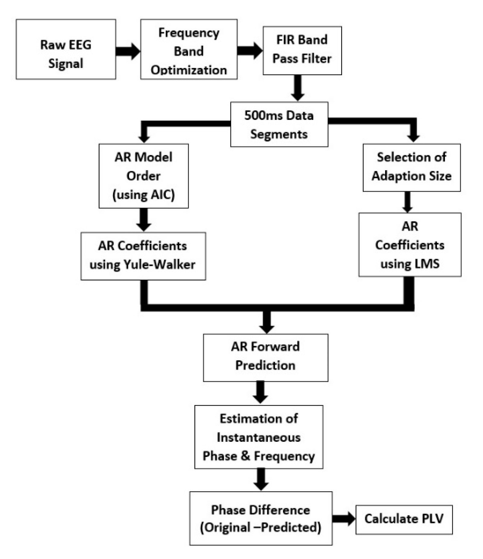
• Re-reference the raw data and then downsample to 500 Hz.
• Optimize the frequency band (8–13 Hz) based on the peak/central frequency of each individual. The individual alpha frequency (IAF) is linked to the maximum EEG power within the alpha range. After finding the IAF, a passband for a band-pass filter is chosen. The low cutoff frequency for the band-pass filter is IAF-1 and high cutoff frequency is IAF+1.
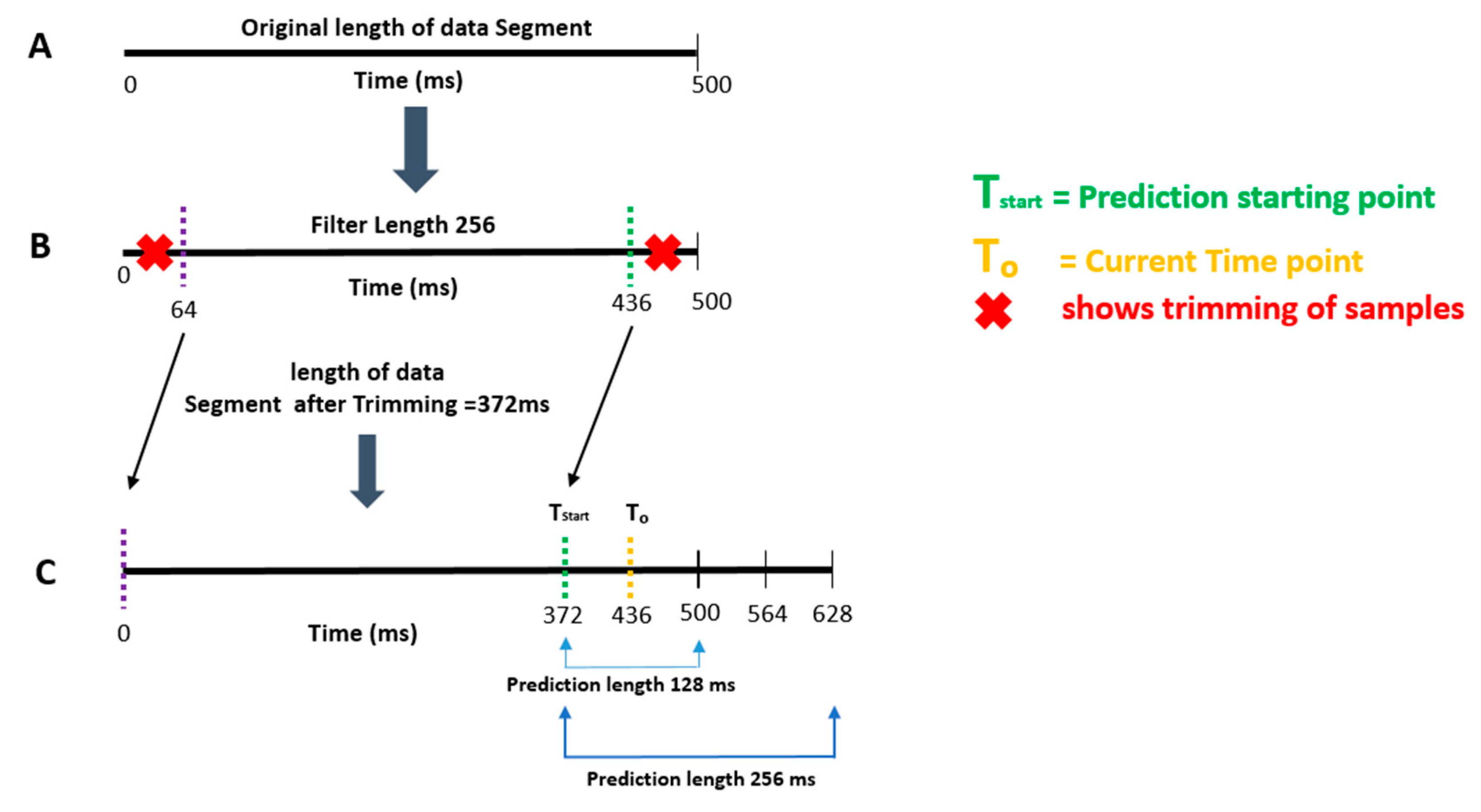
• Apply a two-pass finite impulse response (FIR) band-pass filter with a filter order of 128 and the passband chosen in step 2 [28].
• Segment the data into 500 ms epochs.

AR model (replicating Zrenner’s method) [27]:

• Compute the optimal AR model order using Akaike’s Information Criterion (AIC).
• Compute AR coefficients using the Yule–Walker equations.
• Estimate the instantaneous phase at the boundary of the sliding window in the AR forward prediction method (prediction length, 128 ms) [21,27] (see Figure 1).

LMS-based AR model:

• Select the adaptation size/learning rate of LMS.
• Select the number of filter taps (same as the AR model order).
• Compute the coefficients using LMS and then use those coefficients to predict the next sample until the prediction length in the AR equation.
• Calculate the time-series forward prediction for twice the prediction length (256 ms) for the LMS-based AR model (See Figure 1).

Assessment of performance of AR model and LMS-based AR model:

• Compute the means of the predicted segment and original segment and subtract the respective means from the predicted segment and original segment.
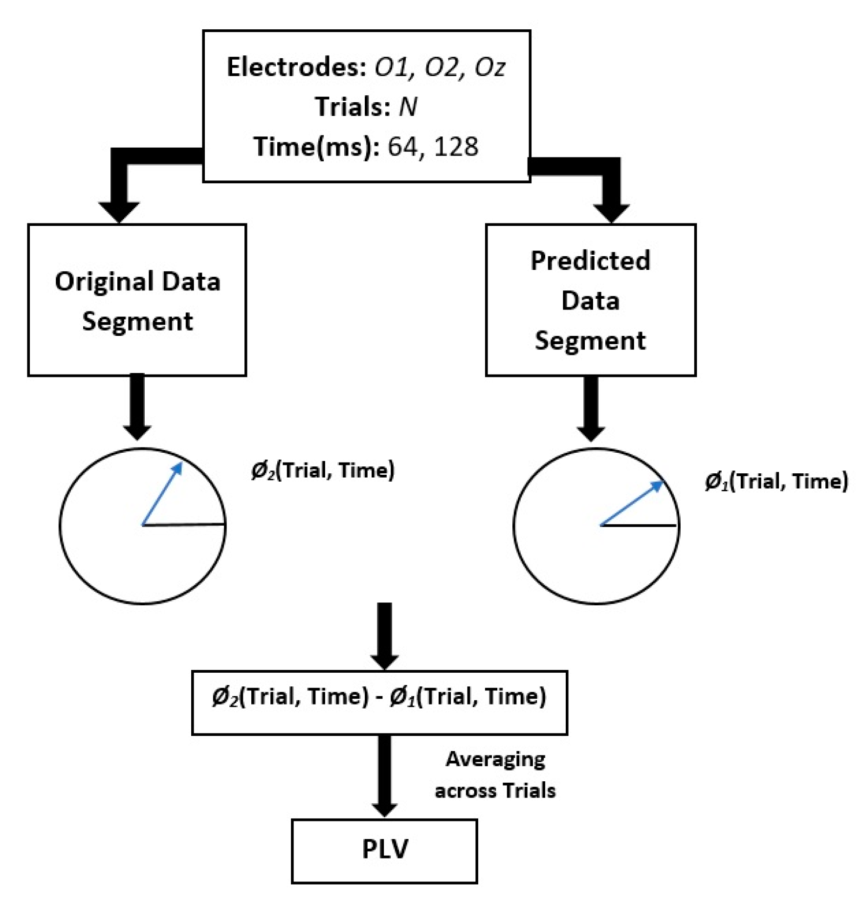
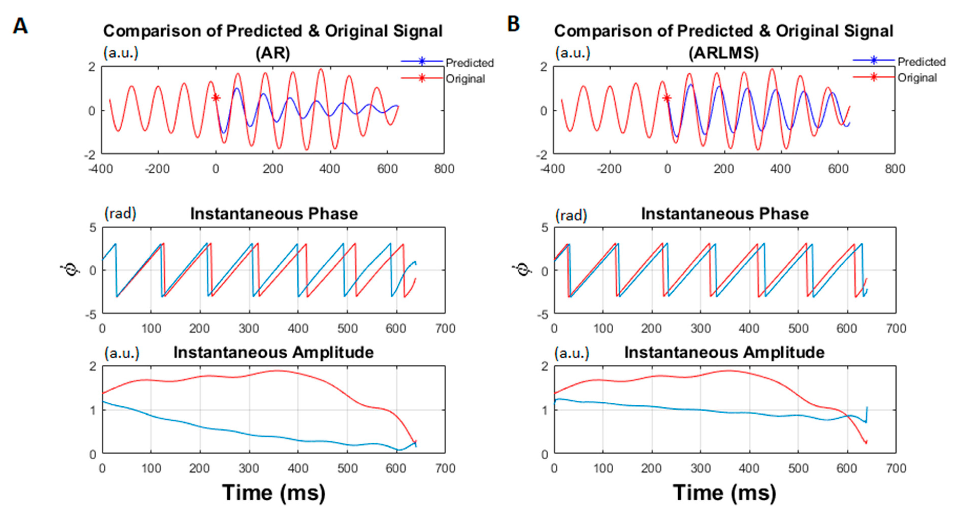
• Estimate the instantaneous phase and frequency of the original and predicted data segments by calculating the analytic signal via the Hilbert transform.
• Compute the phase difference between the original and predicted data segments.
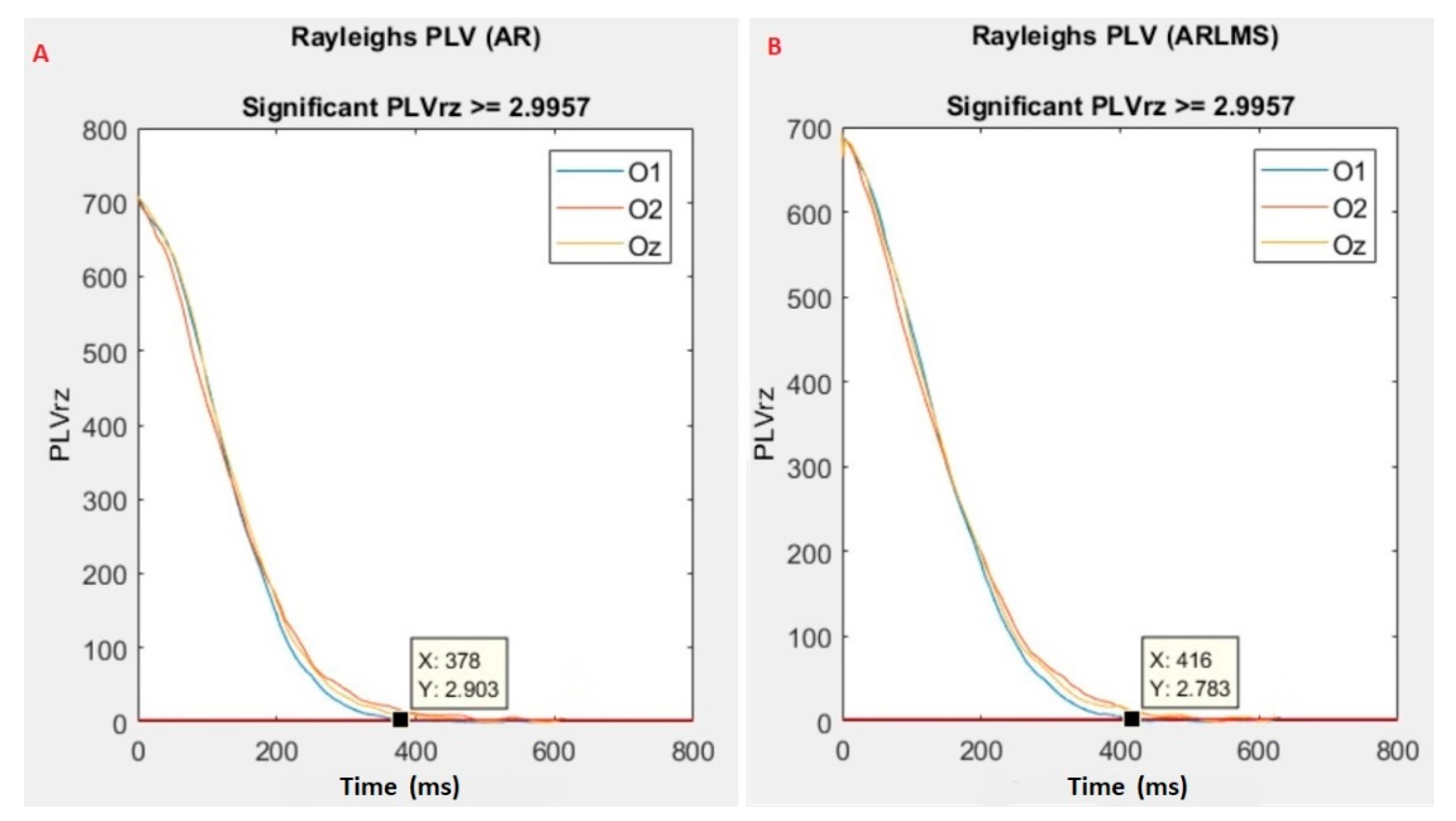
• Calculate the phase locking value (PLV) between the original and predicted data.

The last four steps are to be performed for both methods. A flow chart of these steps is shown in Figure 2.

2.2. Autoregressive (AR) Model

AR modelling has been successfully applied to EEG signal analysis for diverse applications such as segmentation, forecasting, rejection of artifacts [29,30], and speech analysis [31,32]. The AR model is a robust method for estimating the power spectrum of shorter EEG segments and is less susceptible to spurious results [30].

An AR(p) of order p is a random process defined as follows [21]:

$$x\left(n\right)=c+{\displaystyle \sum }_{k=1}^p{\alpha }_{k }x\left(n-k\right)+{\epsilon }_n$$

(1)

where $x\left(n\right)$ is an input data at sample n, $c$ is a constant, ${\alpha }_1$, …, ${\alpha }_p$ are the coefficients of the AR model, and ${\epsilon }_n$ is white noise at sample n.

The AR model can be created using one of numerous algorithms to calculate model coefficients. These algorithms include the Burg lattice method to solve the lattice filter equations, utilizing the mean of backward- and forward-squared prediction errors and the Yule–Walker method to minimize the forward prediction error only. To enable comparisons with previous studies [21,27], we used the Yule–Walker method. The AR model order was selected using Akaike’s Information Criterion (AIC) [33].

2.3. Least Mean Square (LMS)

For a random signal, the main objective of the AR modelling technique is to find recursively the optimal coefficients that minimize the mean square error (MSE) [34]. The LMS algorithm was developed by Hoff and Widrow in 1960 [35]. It employs a stochastic gradient algorithm to solve the least square problem. This method is obtained from steepest-descent implementation by replacing the required gradient vectors and Hessian matrices by more suitable approximations. The equations that constitute the adaptive LMS algorithm are as follows [36]:

$$\mathit{x}\left(n\right)={\left[x\left(n\right), x\left(n-1\right), x\left(n-2\right),\dots x\left(n-M+1\right)\right]}^T$$

(2)

$$\mathit{w}\left(n\right)={\left[w_0\left(n\right), w_1\left(n\right),\dots w_{M-1} \left(n\right)\right]}^T$$

(3)

$$y\left(n\right)={\mathit{w}}^T\left(n\right) \mathit{x}\left(n\right)$$

(4)

$$e\left(n\right)=x\left(n+1\right)-y\left(n\right)$$

(5)

$$\mathit{w}\left(n+1\right)=\mathit{w}\left(n\right)+2\mu e\left(n\right)\mathit{x}\left(n\right)$$

(6)

where $\mathit{x}\left(n\right)$ is an input data at sample n, $y\left(n\right)$ is output, $e\left(n\right)$ is error, $\mathit{w}\left(n\right)$ is filter weight, $\mu$ is step size, and $M$ is filter length.

In the current study, two methods were implemented and compared for time-series forward prediction; first Yule–Walker based AR model and second LMS-based AR model. The AR model computes AR coefficients once, whereas the LMS-based AR model computes them at each instant. The LMS-based AR model algorithm starts from an initial condition without having the desired information and then updates the filter weights based on the input data sequence. The filter length for the LMS-based AR model is the same as for the AR model order.

2.4. Instantaneous Frequency and Phase

The analytic signal is constructed by combining the original data and its Hilbert transform to calculate the instantaneous phase [37]. The complex signal $z_x\left(t\right)$ can be constructed as follows:

$$z_x\left(t\right)=x\left(t\right)+iH\left\{x\left(t\right)\right\}$$

(7)

where $x\left(t\right)$ is the original real signal, and $H\left\{x\left(t\right)\right\}$ is the Hilbert transform of the real signal $x\left(t\right)$ defined as follows:

$$H\left\{x\left(t\right)\right\}=\frac{1}{\pi } p.v. {{\displaystyle \int }}_{-\infty }^{\infty }\frac{x\left(\tau \right)}{t-\tau } d\tau$$

(8)

where $p.v.$ denotes Cauchy’s principal value. The instantaneous phase of the signal can be calculated from the complex analytic signal as follows:

$${\phi }_x\left(t\right)=arg{z}_x\left(t\right)$$

(9)

The instantaneous frequency can then be calculated from the instantaneous phase as follows:

$$f_x\left(t\right)=\frac{1}{2\pi } \frac{d}{dt} {\phi }_x^{uw}\left(t\right)$$

(10)

where ${\phi }_x^{uw}\left(t\right)$ is the unwrapped instantaneous phase.

To estimate the instantaneous phase at the edge of the sliding data segment of 500 ms and to avoid edge effects, 64 ms segments were trimmed on both ends. The remaining 372 ms data segment was then introduced into the AR model to generate AR coefficients. The AR model order was fixed to 30 to iteratively forecast the 128 ms in the future [21]. The predicted 128 ms window was then used to calculate the analytic signal based on the Hilbert transform. As suggested by Zrenner [23], there is a trade-off between the length of the predicted segment and the efficacy of the filter. This study used a 128th order two-pass FIR band pass filter. A higher filter order delays the signal longer, whereas a low filter order <100 does not remove frequencies outside the passband effectively. For the LMS-based AR model, the same, and twice (256 ms) prediction lengths were compared with the AR model.

2.5. Participants

A total of 21 volunteers (10 males and 11 females; mean age + SD, 26.2 + 7.1) were recruited to this study and provided informed consent for EEG analysis before they participated in the study. To record EEG data, participants were asked to rest with their eyes closed while their EEG signals were measured for 3 minutes. The study was conducted in accordance with the Declaration of Helsinki, and the study was approved by the ethics committee of RIKEN (Wako3 26-24). The EEG data had been used in our previous studies for different purposes [38,39,40].

2.6. EEG Recording and Preprocessing

EEG signals were recorded using an EEG amplifier (BrainAmp MR+, Brain Products GmbH, Gilching, Germany) at a sampling rate of 1000 Hz using a 63-channel EEG cap (Easycap, EASYCAP GmbH, Herrsching, Germany). Online low and high cutoff frequencies of the EEG amplifier were set to 0.016 and 250 Hz, respectively. Electrodes were positioned according to the 10/10 system with electrode AFz as the ground electrode and left earlobe as the reference electrode. EEG signals were re-referenced to the average of the right and left earlobe and down sampled to 500 Hz offline. All analysis was performed in MATLAB (Math-Works Inc., Natick, MA, USA) using custom-written scripts and EEGLAB [41].

2.7. Statistical Analysis

All statistical analyses were conducted using MATLAB Statistics and Machine Learning Toolbox. The statistical significance level was set at p < 0.05.

3. Results

The ultimate goal of this study was to replicate the AR model for time-series forward prediction and compare the results with those of the adaptive LMS-based AR model with twice the prediction length. First, we wanted to determine the performance of both methods to assess the phase-locking value (PLV) at different time points [42].

For a given data segment, the difference between the original instantaneous phase and predicted instantaneous phase was computed as shown in Figure 3. The measure yields a number between 0 and 1: with 0 reflecting the high phase variability, and 1 reflecting trials with identical phase. PLV is defined as follows:

$$PLV\left(n\right)=\frac{1}{N}\left|{\displaystyle \sum }_{m=1}^N{e}^{i\left({\varnothing }_2\left(m,n\right)-{\varnothing }_1\left(m,n\right)\right)}\right|$$

(11)

where N is the total number of trials, m is the trial index, Ø₂ is the instantaneous phase of the original data segment, Ø₁ is the instantaneous phase of the predicted data segment, and n is the time.

The statistical significance of the PLV can be tested by calculating Rayleigh’s Z value [43] as follows:

$$Z=NPL{V}^2$$

(12)

where $N$ is the total number of trials.

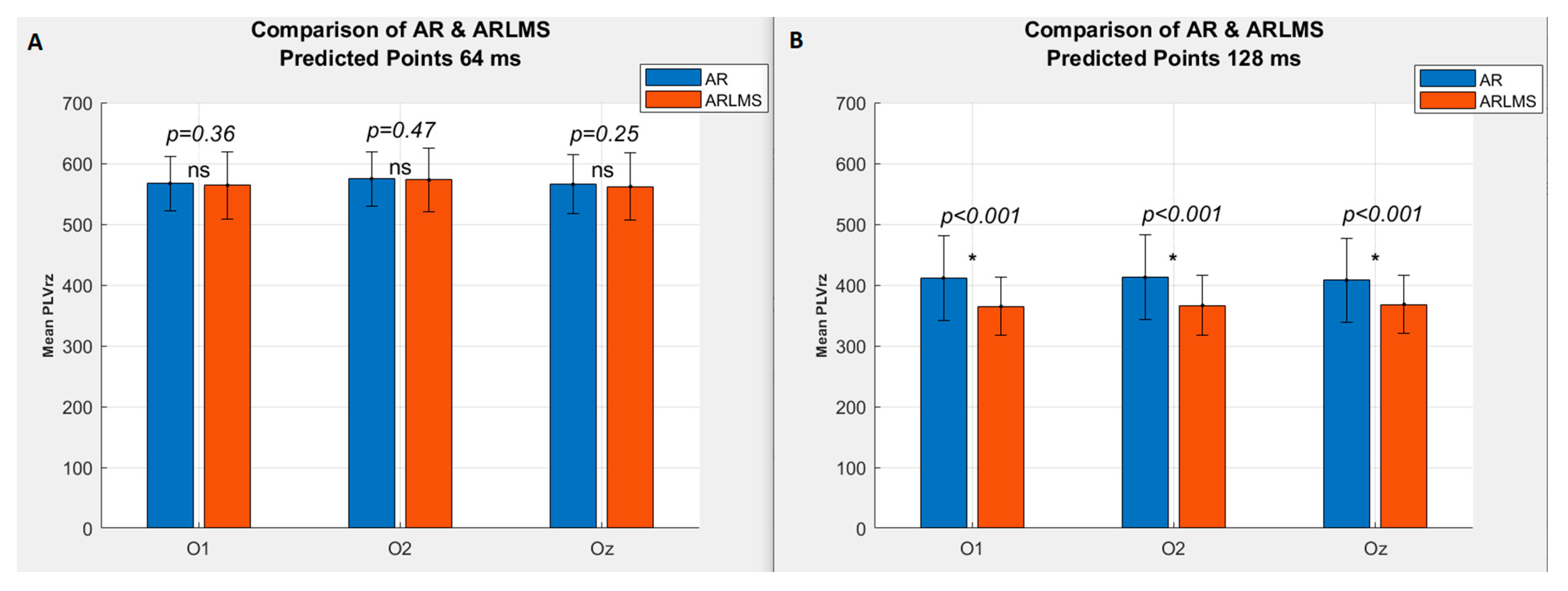
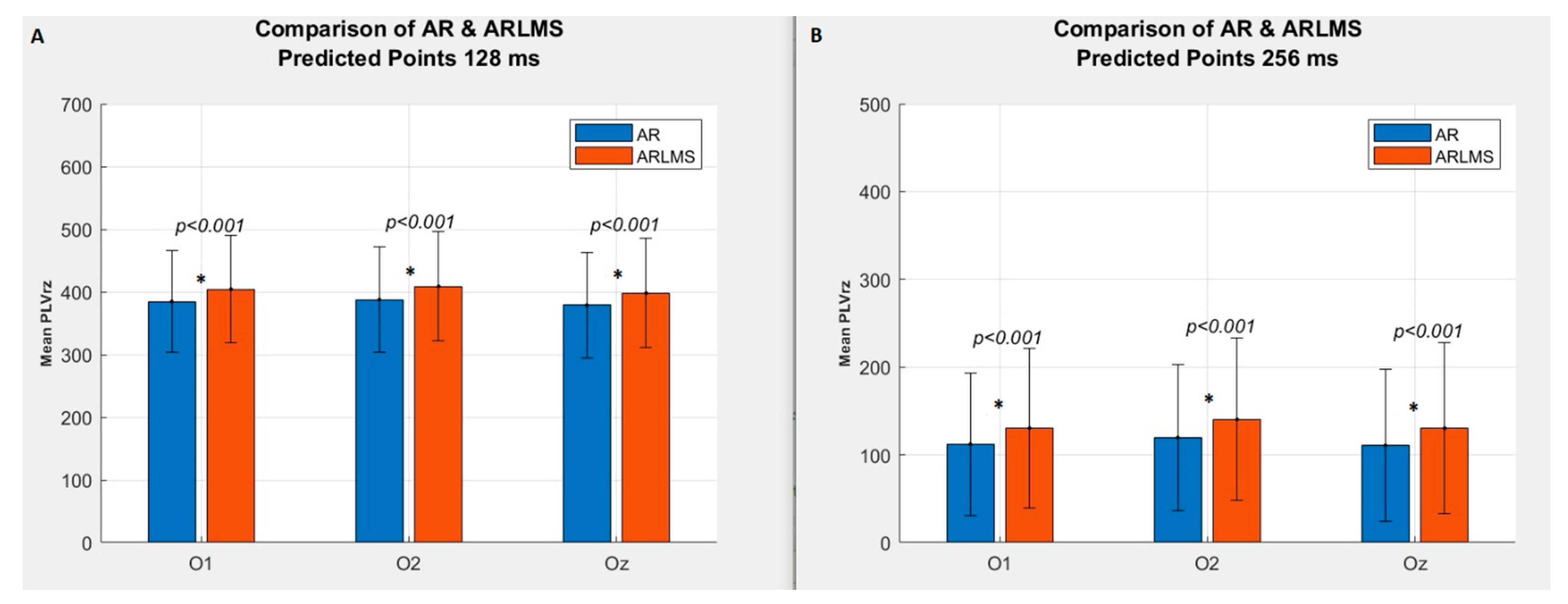
3.1. Shorter Prediction Length

A paired t-test was used to compare the results of both methods for three different channels (O1, O2, and Oz) at two time points (64 ms and 128 ms). Figure 4 depicts the mean values of Rayleigh’s Z value (PLVrz) for all the subjects. Part A shows the results for the AR model, and part B reflects the PLVrz values of the LMS-based AR model. The PLVrz decays slowly, indicating that the prediction performance decreases with time. At 128 ms, there is a significant difference between the two methods where the AR performs better than the LMS-based AR model. For approximately 700 trials per subject across 21 subjects, PLVrz > 2.9957 is considered statistically significant with respect to the p < 0.05 significance level.

3.2. Twice Prediction Length

To investigate how well both methods perform with increasing prediction length, the prediction length was increased twice (256 ms: 128 samples). The prediction performance usually decays with time [44]. However, the LMS-based AR model showed better prediction performance when the length was increased, as shown in Figure 5.

Representative PLVrz values as a function of predicted time points are shown for three channels (O1, O2, and Oz) in Figure 6. Both parts of the figure show a decay with respect to increasing prediction length and crossing the significance line. For this particular subject, the AR model shows the 378 ms (189th sample) for crossing, while the LMS-based AR model shows the 416 ms (208th sample) for crossing the significant line.

Both methods were compared using a paired t-test for three channels: O1, O2, and Oz. At 128 ms and the 256 ms, the LMS-based AR model showed higher PLVrz than the AR model. Although the performance of both methods declined with increasing prediction length, the LMS-based AR model outperformed the AR model when the length was increased two times, as shown by their mean PLV Rayleigh Z values (Figure 7).

3.3. Sampling Points Crossing the Significant Rayleigh’s Z Value

Next, we investigated which of the sampling points in the 800 ms interval per individual subject crossed the significant Rayleigh’s Z value (>2.9957). When the prediction length was increased to 800 ms, the performance of both methods declined (

Table 1. Time points crossing the significant Rayleigh’s PLV for channel O1 for both the autoregressive (AR) model and the least mean square (LMS)-based AR model. Asterisk (*) means that out of 800 ms, the particular channel did not cross the significant value (>2.9957).

Subjects	Results of Channel O1 800 ms
	Autoregressive (AR) Model	Least Mean Square (LMS)-based AR Model
	Time Points	Time Points
1.	424	446
2.	368	392
3.	536	550
4.	492	484
5.	382	416
6.	420	578
7.	452	456
8.	678	752
9.	392	370
10.	694	*
11.	630	678
12.	506	556
13.	702	618
14.	524	522
15.	796	*
16.	644	598
17.	528	578
18.	*	778
19.	566	598
20.	660	714
21.	452	406

). Amongst the 21 participants, 15 subjects showed higher crossing values with the LMS-based AR model than with the AR model. A significant difference was observed between the two methods for time points <400 (

Table 2. Statistical comparison of Rayleigh’s Z value for channel O1 for 800 ms prediction.

Prediction Time Point (ms)	p-Value	AR Model	LMS-Based AR Model
		Rayleigh’s Z Value (Mean Values)
64	p < 0.001	582	568
128	p < 0.001	384	403
256	p < 0.001	113	131
340	p = 0.010	50.5	61.18
400	p = 0.070	29	35

). At 64 ms, the AR model surpassed the LMS-based AR model, whereas for the 128 ms, 256 ms, and 340 ms, the LMS-based AR model outperformed the AR model. For time points greater than 400 ms, there was no significant difference between the two methods, and their performances declined.

4. Discussion

Estimation of the phase of EEG rhythms is challenging due to their low signal-to-noise ratio and dynamic nature. In this study, we presented an adaptive method to estimate the phase of alpha oscillations and compared the results with those of the AR model. Our aim was to improve real-time EEG applications that depend on phase estimates. This approach estimates instantaneous frequency and phase of an EEG segment (three channels: O1, O2, and Oz) and then forecasts the signal based on these aforementioned methods. Two prediction lengths (128 ms and 256 ms) of the EEG segment were investigated, and performance was evaluated in terms of PLV.

Previously, Zrenner [27] used the AR model [21]. For comparison and consistency purposes, we applied the AR model with the same filtering method, AR model order, length of EEG data segment, and prediction length. Additionally, we assessed how the future prediction window affected the performance of both methods. Earlier studies used the Hilbert–Huang transform [45,46] and complex wavelet transform [47] to extract frequency and phase information from EEG signals. These methods are limited because the task of predicting a future signal is hard to resolve using analysis of non-stationary data. Rendering methods such as AR assume stationarity over short time periods, therefore they are not suitable for closed- loop and real-time applications. Our adaptive method relies on frequent updates to cater for EEG signals with non-stationarity, thus making it possible to predict the future signal while adjusting to dynamic changes over time.

Considering the precise phase dynamics of an ongoing oscillation, the use of closed-loop neurostimulation has escalated significantly in the last few years. Specifically, a prior study [48] used Fast Fourier- and Hilbert transform-based algorithms for phase-locked stimulation of different EEG bands. The authors proposed a short window prediction algorithm based on an intermittent protocol with distinct windows for phase extraction and prediction. As in our study, they used the PLV metric for performance evaluation and exceeded it to 0.6 for alpha band detection. Similarly, they reported that performance declined relative to increasing the size of prediction length in both methods. The major limitations of this study were a relatively small sample size and neglect to show the functioning of a whole closed-loop system. A study published in 2018 reported three different phase prediction methods (AR model, Hilbert-based, and zero crossing) [44]. Different performance metrics were applied, including PLV, phase synchrony based on entropy, and degree deviation. Their study confirmed that PLV decreases with an increasing time-window as indicated by an increase in alpha fluctuations at longer intervals. Drawbacks of the study include a small sample size (eight), use of only one channel (Oz), and failure to determine whether the AR or Hilbert-based methods were optimal.

Most studies estimate the phase based on standard signal processing methods. Recently machine learning techniques, specifically deep learning methods, have been implemented in many BCI systems. An eleven layered Convolutional Neural Network (CNN) model was used to detect schizophrenia [49]. High classification accuracy 81% for the subject and 98% for non-subject based testing were achieved. Despite high classification accuracies, the major limitations include small data pool, and CNN is costly to compute as compared to traditional machine learning algorithms. CNN was also implemented in an automated detection system for Parkinson’s disease with an accuracy of 88.25% [50]. Another study employed Principal Component Analysis (PCA)-based CNN for p300 EEG signals [51]. PCA was used to reduce the dimension of the signal and computational cost by retaining the data features of the original signal. A combination of the continuous wavelet transform and simplified CNN named SCNN was implemented to enhance the recognition rate of motor imagery EEG signals [52]. Compared with CNN, the SCNN shortens the training time and reduces the parameters; however, the classification accuracy needs to be improved. An interesting study implemented the deep learning algorithm in neuromarketing utilizing EEG signals for a product-based preference detection. Although the deep neural network produced good results, a random forest algorithm yields similar results on the same dataset [53]. Two-level cascaded CNN was proposed to detect the stego texts generated by substituting synonyms [54]. The proposed steganalysis algorithms showed enhanced prediction performance with an accuracy of 82.2%. A study investigated machine-learning methods to extract the instantaneous phase of an EEG signal centered at POz [55]. Similar to our study, the authors also performed frequency band optimization based on individual alpha frequency. To compose analytic signals, the algorithm was split into two branches: on the first path, to generate an input signal, data were epoched only, and on the second path, to generate an output signal, an FIR band-pass filter was applied on the data. The second path was directly followed by Hilbert transform and then epoching as the last step before evaluation of the model. The data was trained with an optimized filter, and instantaneous phase recovered via application of the Hilbert transform and non-causal filtering to minimize MSE. The main disadvantage of this procedure is the need for preliminary data prior to the principal experiment for training purposes. Since real-time phase estimation does not provide future information, the trained filters depend on the quality of the signal and their underlying properties. As a result, this method does not assume unbiased phase estimation. Although deep learning techniques are highly efficient, they require a copious amount of data for training. Another challenge is that it requires a huge amount of processing power and, therefore, is a costly affair.

Recently, databases comprising abundant similar time-series have been available for many applications. For such data, utilizing traditional univariate methods in time-series forecasting leaves a great possibility for generating a precise forecast unexploited. A comprehensive review article sheds light on utilizing CNN, Long Short Term Memory (LSTM), and Deep Belief Networks for financial time-series forecasting [56]. Recently, recurrent neural networks, particularly LSTM networks, have proven to be able to surpass the traditional state-of-the-art time-series forecasting methods. LSTM has attracted much attention and has been widely used in various domains in data science such as forecasting of the production rate of petroleum oil [57], wind speed forecasting [58], weather forecasting [59], and speech recognition [60]. Although the accuracy of the methods, as mentioned above, may decline in the presence of the heterogeneous time-series data [61], we need to further investigate the possibility of using such recent techniques, which have been applied to other data types already mentioned.

The goal of this study was to estimate the EEG signal phase by utilizing an adaptive method. In support of earlier studies, our results clearly show that for longer prediction intervals, the LMS-based AR model outperforms the AR model. Even for single channel O1, the LMS-based AR model shows higher samples crossing the significance line. Our proposed method may also be deployed as an alternative to the AR model, when longer prediction length is the key. The LMS-based AR model offers a feasible approach for mimicking the results of previous studies while incurring faster adaptation to the underlying EEG signal at lower computational costs. Limitations of the current study include the need to apply (a) the proposed method for different EEG rhythms, (b) performance evaluation in some behavioral tasks (rather than a simple case of resting state), and (c) single performance metric (i.e., PLV). Further work will involve overcoming the limitations and implementation in a real-time scenario, such as by closed-loop stimulation or exploring new vistas for alpha oscillations.

5. Conclusions

Our analytical approach to estimate EEG phase relies on instantaneous alpha oscillations using the conventional Yule–Walker-based method (AR) and the adaptive method (LMS). The LMS-based AR model serves at least two main purposes. First, it avoids pre-existing knowledge of the exact signal stochastic, which is rarely available in practice when a learning mechanism is used to estimate the required signal statistics. Second, it possesses a tracking mechanism to monitor the variation in the EEG signal. By comparing these two methods, our study showed that the adaptive LMS-based AR model outperforms the AR model in real time for longer prediction lengths. This new approach may raise the possibility of EEG phase prediction with its simplicity and low computational cost. In summary, our proposed technique can help in neurostimulation applications, such as EEG phase prediction aids in versatile brain-machine interface applications.

References

1. Womelsdorf, T.; Schoffelen, J. Modulation of neuronal interactions through neuronal synchronization. Science 2007, 316, 1609–1612. [Google Scholar] [CrossRef] [PubMed] [Green Version]
2. Mathewson, K.E.; Lleras, A. Pulsed out of awareness: EEG alpha oscillations represent a pulsed- inhibition of ongoing cortical processing. Front. Psychol. 2011, 2, 99. [Google Scholar] [CrossRef] [PubMed] [Green Version]
3. Klimesch, W.; Sauseng, P. EEG alpha oscillations: The inhibition–timing hypothesis. Brain. Res. Rev. 2007, 53, 63–88. [Google Scholar] [CrossRef] [PubMed]
4. Jensen, O.; Mazaheri, A. Shaping functional architecture by oscillatory alpha activity: Gating by inhibition. Front. Hum. Neurosci. 2010, 4, 186. [Google Scholar] [CrossRef] [Green Version]
5. Thut, G.; Nietzel, A. α-Band electroencephalographic activity over occipital cortex indexes visuospatial attention bias and predicts visual target detection. J. Neurosci. 2006, 26, 9494–9502. [Google Scholar] [CrossRef] [Green Version]
6. Gratton, G.; Villa, A.E.P. Functional correlates of a three-component spatial model of the alpha rhythm. Brain Res. 1992, 582, 159–162. [Google Scholar] [CrossRef]
7. Worden, M.S.; Foxe, J. Anticipatory biasing of visuospatial attention indexed by retinotopically specific-band electroencephalography increases over occipital cortex. J. Neurosci. 2000, 20, 63. [Google Scholar] [CrossRef] [Green Version]
8. Pfurtscheller, G.; Neuper, C. Event-related synchronization of mu rhythm in the EEG over the cortical hand area in man. Neurosci. Lett. 1994, 174, 93–96. [Google Scholar] [CrossRef]
9. Hanslmayr, S.; Aslan, A. Prestimulus oscillations predict visual perception performance between and within subjects. Neuroimage 2007, 37, 1465–1473. [Google Scholar] [CrossRef]
10. Van Dijk, H.; Schoffelen, J. Prestimulus oscillatory activity in the alpha band predicts visual discrimination ability. J. Neurosci. 2008, 28, 1816–1823. [Google Scholar] [CrossRef] [Green Version]
11. Lerga, J.; Saulig, N.; Mozetic, V.; Lerga, R. Number of EEG signal components estimated using the short-term Rényi entropy. In Proceedings of the 2016 International Multidisciplinary Conference on Computer and Energy Science (SpliTech), Split, Croatia, 13–15 July 2016. [Google Scholar]
12. Lerga, J.; Saulig, N. Algorithm based on the short-term Rényi entropy and IF estimation for noisy EEG signals analysis. Comput. Biol. Med. 2017, 80, 1–13. [Google Scholar] [CrossRef]
13. Jadav, G.M.; Lerga, J. Adaptive filtering and analysis of EEG signals in the time-frequency domain based on the local entropy. EURASIP J. Adv. Signal Process. 2020, 2020, 1–18. [Google Scholar]
14. Khan, N.A.; Mohammadi, M.; Ali, S. Instantaneous frequency estimation of intersecting and close multi-component signals with varying amplitudes. Signal Image Video Process. 2019, 13, 517–524. [Google Scholar] [CrossRef]
15. Mathewson, K.E.; Gratton, G. To see or not to see: Prestimulus α phase predicts visual awareness. J. Neurosci. 2009, 29, 2725–2732. [Google Scholar] [CrossRef] [PubMed] [Green Version]
16. VanRullen, R.; Busch, N. Ongoing EEG phase as a trial-by-trial predictor of perceptual and attentional variability. Front. Psychol. 2011, 2, 60. [Google Scholar] [CrossRef] [Green Version]
17. Busch, N.A.; Dubois, J. The phase of ongoing EEG oscillations predicts visual perception. J. Neurosci. 2009, 29, 7869–7876. [Google Scholar] [CrossRef] [PubMed]
18. Pavlides, C.; Greenstein, Y.J. Long-term potentiation in the dentate gyrus is induced preferentially on the positive phase of θ-rhythm. Brain Res. 1988, 439, 383–387. [Google Scholar] [CrossRef]
19. Hölscher, C.; Anwyl, R. Stimulation on the positive phase of hippocampal theta rhythm induces long-term potentiation that can be depotentiated by stimulation on the negative phase in area CA1 in vivo. J. Neurosci. 1997, 17, 6470–6477. [Google Scholar] [CrossRef]
20. Hyman, J.M.; Wyble, B.P. Stimulation in hippocampal region CA1 in behaving rats yields long-term potentiation when delivered to the peak of theta and long-term depression when delivered to the trough. J. Neurosci. 2003, 23, 11725–11731. [Google Scholar] [CrossRef]
21. Chen, L.L.; Madhavan, R. Real-time brain oscillation detection and phase-locked stimulation using autoregressive spectral estimation and time-series forward prediction. IEEE Trans. Biomed. Eng. 2011, 60, 753–762. [Google Scholar] [CrossRef] [Green Version]
22. Roux, S.G.; Cenier, T. A wavelet-based method for local phase extraction from a multi-frequency oscillatory signal. J. Neurosci. Methods 2007, 160, 135–143. [Google Scholar] [CrossRef] [PubMed] [Green Version]
23. Brunner, C.; Scherer, R. Online control of a brain-computer interface using phase synchronization. IEEE Trans. Biomed. Eng. 2006, 53, 2501–2506. [Google Scholar] [CrossRef] [PubMed]
24. Marzullo, T.C.; Lehmkuhle, M.J. Development of closed-loop neural interface technology in a rat model: Combining motor cortex operant conditioning with visual cortex microstimulation. IEEE Trans. Neural Syst. Rehabil. Eng. 2010, 18, 117–126. [Google Scholar] [CrossRef] [PubMed] [Green Version]
25. Anderson, W.S.; Kossoff, E.H. Implantation of a responsive neurostimulator device in patients with refractory epilepsy. Neurosurg. Focus 2008, 25, E12. [Google Scholar] [CrossRef] [PubMed]
26. Anderson, W.S.; Kudela, P. Phase-dependent stimulation effects on bursting activity in a neural network cortical simulation. Epilepsy. Res. 2009, 84, 42–55. [Google Scholar] [CrossRef] [Green Version]
27. Zrenner, C.; Desideri, D. Real-time EEG-defined excitability states determine efficacy of TMS-induced plasticity in human motor cortex. Brain Stimul. 2018, 11, 374–389. [Google Scholar] [CrossRef]
28. Schaworonkow, N.; Triesch, J. EEG-triggered TMS reveals stronger brain state-dependent modulation of motor evoked potentials at weaker stimulation intensities. Brain Stimul. 2019, 12, 110–118. [Google Scholar] [CrossRef]
29. Tseng, S.-Y.; Chen, R.-C. Evaluation of parametric methods in EEG signal analysis. Med. Eng. Phys. 1995, 17, 71–78. [Google Scholar] [CrossRef]
30. Pardey, J.; Roberts, S.; Tarassenko, L. A review of parametric modelling techniques for EEG analysis. Med. Eng. Phys. 1996, 18, 2–11. [Google Scholar] [CrossRef]
31. Koo, B.; Gibson, J.D.; Gray, S.D. Filtering of colored noise for speech enhancement and coding. In Proceedings of the International Conference on Acoustics, Speech, and Signal Processing, Glasgow, UK, 23–26 May 1989. [Google Scholar] [CrossRef]
32. Lim, J.; Oppenheim, A. All-pole modeling of degraded speech. IEEE Trans. Signal. Process. 1978, 26, 197–210. [Google Scholar] [CrossRef]
33. Akaike, H. A new look at the statistical model identification. IEEE Trans. Autom. Control 1978, 19, 465–471. [Google Scholar] [CrossRef]
34. Wu, W.R.; Chen, P.C. Adaptive AR modeling in white Gaussian noise. IEEE Trans. Signal Process. 1997, 45, 1184–1192. [Google Scholar] [CrossRef]
35. Widrow, B.; Stearns, D.S. Adaptive Signal Processing, 1st ed.; Prentice-Hall, Inc.: Upper Saddle River, NJ, USA, 1985. [Google Scholar]
36. Poularikas, A.D.; Ramadan, Z.M. Adaptive Filtering Primer with MATLAB, 1st ed.; CRC Press: Boca Raton, FL, USA, 2006; pp. 101–135. [Google Scholar]
37. Boashash, B. Estimating and interpreting the instantaneous frequency of a signal. I. Fundamentals. Proc. IEEE 1992, 80, 520–538. [Google Scholar] [CrossRef]
38. Suetani, H.; Kitajo, K. A manifold learning approach to mapping individuality of human brain oscillations through beta-divergence. Neurosci. Res. 2020. [Google Scholar] [CrossRef] [PubMed]
39. Kitajo, K.; Sase, T. Consistency in macroscopic human brain responses to noisy time-varying visual inputs. bioRxiv 2019, 645499. [Google Scholar] [CrossRef]
40. Sase, T.; Kitajo, K. The metastable human brain associated with autistic-like traits. bioRxiv 2019, 855502. [Google Scholar] [CrossRef] [Green Version]
41. Delorme, A.; Makeig, S. EEGLAB: An open source toolbox for analysis of single-trial EEG dynamics including independent component analysis. J. Neurosci. Methods 2004, 134, 9–21. [Google Scholar] [CrossRef] [Green Version]
42. Lachaux, J.P.; Rodriguez, E. Measuring phase synchrony in brain signals. Hum. Brain. Mapp. 1999, 8, 194–208. [Google Scholar] [CrossRef] [Green Version]
43. Fischer, N. Statistical Analysis of Circular Data; Cambridge UP: Cambridge, UK, 1993. [Google Scholar] [CrossRef]
44. Zarubin, G.; Gundlach, C. Real-time phase detection for EEG-based tACS closed-loop system. In Proceedings of the 6th International Congress on Neurotechnology, Electronics and Informatics, Seville, Spain, 20–21 Spetember 2018. [Google Scholar] [CrossRef]
45. Bajaj, V.; Pachori, R.B. Separation of rhythms of EEG signals based on Hilbert-Huang transformation with application to seizure detection. In Proceedings of the International Conference on Hybrid Information Technology, Daejeon, Korea, 23–25 August 2012. [Google Scholar] [CrossRef]
46. Lin, C.F.; Zhu, J.D. Hilbert-Huang transformation-based time-frequency analysis methods in biomedical signal applications. Proc. Inst. Mech. Eng. Part H 2012, 226, 208–216. [Google Scholar] [CrossRef]
47. Le Van Quyen, M. Comparison of Hilbert transform and wavelet methods for the analysis of neuronal synchrony. J. Neurosci. Methods 2001, 111, 83–98. [Google Scholar] [CrossRef]
48. Mansouri, F.; Dunlop, K. A fast EEG forecasting algorithm for phase-locked transcranial electrical stimulation of the human brain. Front. Neurosci. 2017, 11, 401. [Google Scholar] [CrossRef] [PubMed] [Green Version]
49. Oh, S.L.; Jahmunah, V. Deep convolutional neural network model for automated diagnosis of schizophrenia using EEG signals. Appli. Sci. 2019, 9, 2870. [Google Scholar] [CrossRef] [Green Version]
50. Oh, S.L.; Hagiwara, Y. A deep learning approach for Parkinson’s disease diagnosis from EEG signals. Neural Comput. Appl. 2018, 1–7. [Google Scholar] [CrossRef]
51. Li, F.; Li, X. A Novel P300 Classification Algorithm Based on a Principal Component Analysis-Convolutional Neural Network. Appli. Sci. 2020, 10, 1546. [Google Scholar] [CrossRef] [Green Version]
52. Li, F.; He, F. A Novel Simplified Convolutional Neural Network Classification Algorithm of Motor Imagery EEG Signals Based on Deep Learning. Appli.Sci. 2020, 10, 1605. [Google Scholar] [CrossRef]
53. Aldayel, M.; Ykhlef, M. Deep Learning for EEG-Based Preference Classification in Neuromarketing. Appl. Sci. 2020, 10, 1525. [Google Scholar] [CrossRef] [Green Version]
54. Xiang, L.; Guoqing, G. A convolutional neural network-based linguistic steganalysis for synonym substitution steganography. Math. Biosci. Eng. 2020, 17, 1041–1058. [Google Scholar] [CrossRef]
55. McIntosh, J.; Sajda, P. Estimation of phase in EEG rhythms for real-time applications. arXiv 2019, arXiv:1910.08784. [Google Scholar]
56. Sezer, O.B.; Gudelek, M.U. Financial time series forecasting with deep learning: A systematic literature review: 2005–2019. Appl. Soft. Comput. 2020, 90, 106181. [Google Scholar] [CrossRef] [Green Version]
57. Song, X.; Liu, Y.; Xue, L. Time-series well performance prediction based on Long Short-Term Memory (LSTM) neural network model. J. Petrol. Sci. Eng. 2020, 186, 106682. [Google Scholar] [CrossRef]
58. Memarzadeh, G.; Keynia, F. A new short-term wind speed forecasting method based on fine-tuned LSTM neural network and optimal input sets. Energ. Convers. Manag. 2020, 213, 112824. [Google Scholar] [CrossRef]
59. Karevan, Z.; Suykens, J.A.K. Transductive LSTM for time-series prediction: An application to weather forecasting. Neural Netw. 2020, 125, 1–9. [Google Scholar] [CrossRef] [PubMed]
60. Monesi, M.J.; Accou, B.; Martinez, J.M.; Francart, T.; Hamme, H.V. An LSTM Based Architecture to Relate Speech Stimulus to EEG. arXiv 2020, arXiv:2002.10988. [Google Scholar]
61. Bandara, K.; Bergmeir, C.; Smyl, S. Forecasting across time series databases using recurrent neural networks on groups of similar series: A clustering approach. Expert. Sys. Appl. 2020, 140, 112896. [Google Scholar] [CrossRef] [Green Version]
Figure 1. Autoregressive (AR) forward prediction. (A) The length of the actual data segment is 500 ms; (B) From both ends, a 64 ms data segment was trimmed; (C) The remaining 372 ms data segment was used to generate AR coefficients to forecast 128 and 256 ms data segment.
Applsci 10 03616 g001
Figure 2. Algorithm Overview. The flow chart shows the sequential steps. The first four steps and the last four steps are the same for both the AR model and the least mean square (LMS)-based AR model.
Applsci 10 03616 g002
Figure 3. Diagram of calculation method of phase-locking value (PLV) [42] between origanl and predicted data segments. Intertrial variability of phase differences between the original and predicted data segments from the same electrodes was calculated. PLV was calculated for three different electrodes (O1, O2, and Oz) and at three different time points (0, 128, 256 ms), respectively.
Applsci 10 03616 g003
Figure 4. Rayleigh’s PLV for the AR model and the LMS-based AR model, ns represents not significant p-value while Asterisk (*) indicates significant p-value. (A) Mean of Rayleigh’s Z value (PLVrz) at the current time point (64 ms); (B) Mean PLVrz at the 128 ms. Error bars indicate the standard deviation of the mean.
Applsci 10 03616 g004
Figure 5. Representative prediction data of the AR model and the LMS-based AR model for double the prediction length (256 ms). Original data segment is shown as the red signal, while the predicted signal is shown in blue. (A) AR model and its respective instantaneous phase and amplitude; (B) LMS-based AR model and its corresponding instantaneous phase and amplitude. Asterisk (*) shows the prediction starting point.
Applsci 10 03616 g005
Figure 6. Rayleigh’s Z value (PLVrz) for twice the prediction length (256 ms). (A) shows the AR model; (B) shows the LMS-based AR model. The red line indicates the significance level with a value of 2.9957. The box shows the time point (X-axis) at which the significant line is crossed with its respective PLVrz value (Y-axis).
Applsci 10 03616 g006
Figure 7. Statistical Comparison of the AR model and the LMS-based AR model for the twice prediction length (256 ms). Asterisk (*) shows significant p-value. (A) Mean PLVrz at 128 ms; (B) Mean PLVrz at 256 ms. Error bars indicate the standard deviation of mean.
Applsci 10 03616 g007