Empirical Modeling of Liquefied Nitrogen Cooling Impact during Machining Inconel 718

Featured Application

Implementation of a machine learning procedure to model the temperature drop in the cryogenic cooling of Inconel 718. Machine learning is performed by an adaptive neuro-fuzzy inference system (ANFIS). Based on a representative set of cryogenic cooling experiments, the formed response surfaces (of temperature drop in Inconel 718) are represented as a set of fuzzy logic rules. Since we are dealing with a small set of experiments (input–output datapoints), the leave one subject out (LOSO) version of k-fold cross-validation is adopted. LOSO offers to exploit the small datasets and by them assess and tune the overall ANFIS modeling performance. A machine learning-based model is designed to minimize the RMSE prediction error by finding the optimal set of hyper-parameters (external ANFIS input parameters). The optimization is performed with the particle swarm optimization (PSO) algorithm.

Abstract

This paper explains liquefied nitrogen’s cooling ability on a nickel super alloy called Inconel 718. A set of experiments was performed where the Inconel 718 plate was cooled by a moving liquefied nitrogen nozzle with changing the input parameters. Based on the experimental data, the empirical model was designed by an adaptive neuro-fuzzy inference system (ANFIS) and optimized with the particle swarm optimization algorithm (PSO), with the aim to predict the cooling rate (temperature) of the used media. The research has shown that the velocity of the nozzle has a significant impact on its cooling ability, among other factors such as depth and distance. Conducted experimental results were used as a learning set for the ANFIS model’s construction and validated via k-fold cross-validation. Optimization of the ANFIS’s external input parameters was also performed with the particle swarm optimization algorithm. The best results achieved by the optimized ANFIS structure had test root mean squared error ($test RMSE)=0.2620$, and $test R^2=0.8585$, proving the high modeling ability of the proposed method. The completed research contributes to knowledge of the field of defining liquefied nitrogen’s cooling ability, which has an impact on the surface characteristics of the machined parts.

1. Introduction

Materials such as high temperature alloys (nickel, titanium, etc.) are usually employed in the manufacturing processes of high added value products, especially in the space, aircraft and military industries [1]. These sorts of materials have excellent mechanical and thermal properties which are maintained even when the materials are exposed to high temperatures. Additionally, such materials have low thermal conductivity and get plastically hardened at high temperatures, hence their extremely poor machinability [2]. The nickel-based alloy Inconel 718, which is the subject of the research in this paper, is a high temperature alloy. It is a corrosion (oxidation) resistant material that can be used at high temperatures while maintaining its hardness characteristics. This is due to its good tensile strength, fatigue life, creep properties and rupture strength. However, due to these specific material characteristics, this alloy is generally difficult to machine [3]. According to these mentioned facts, it could be possible to machine those materials by the usage of cooling lubrication fluids, such as a high-pressure jet and liquefied nitrogen, etc. The development of the industry in the field of machining processes has been striving to achieve a higher level of productivity and environmental awareness. This includes minimizing the use of cooling lubrication fluids based on artificial ingredients and increasing cutting speeds. The use of ecologically impeccable cooling lubrication fluids that do not harm people’s health and are environmentally friendly has been promoted. Thus, it is necessary to use an environmentally acceptable coolant in the manufacturing industry. For this purpose, liquefied nitrogen as a cryogenic coolant has been explored since the 1950s in the metal cutting industry [4]. The main characteristic of this technology is the use of a cryogenic fluid (liquefied nitrogen) as a cooling fluid during the cutting process, at very low temperatures. The main advantage of liquefied nitrogen is the cooling of the cutting zone, where it is the highest temperature. A deficiency of using liquefied nitrogen as cooling fluid during the machining process is a lack of knowledge in terms of the physical properties of the used media and consequently there are very few publications about them in scientific journals.

In past publications on the field of cryogenic machining, artificial intelligence methods were only used to predict machinability aspects: tool wear, cutting forces and surface roughness. In the field of measuring temperatures during the machining process and designing empirical models, the few works are the following. Mozammel and Dhar [5] conducted experiments on measuring temperatures in the hard turning of AISI 1060 steel with coated carbide inserts and developed the predictive empirical model of cutting temperatures with neural networks. Chinchanikar and Choudhury [6] performed experiments on the machining of hardened steel and reached the modeling of the correlations between cutting parameters and different machine aspects including tool wear, chip morphology and surface integrity. Ezugwu et al. [7] reached a correlation between cutting parameters and output process parameters such as tool wear and cutting force in the high speed machining of Inconel 718 with neural networks. Elbaz et al. used a genetic algorithm [8] and particle swarm optimization (PSO) [9] as a learning method of the adaptive neuro-fuzzy inference system (ANFIS) in order to optimize the positions of membership functions (MFs) (making the search space significantly bigger since more independent variables were included in optimization) and increase the ANFIS’s accuracy based on leave out cross-validation.

The aim of the paper is to explain in detail the influence of the characteristic aspects of the placement of the nitrogen inlet on the treatment process. Designing an empirical model can help us to understand the influence of the cooling medium used in the machining process. Within the research, a set of experiments was conducted where the material Inconel 718 was cooled by a moving liquefied nitrogen jet, with the aim of measuring the temperature in the plate. The empirical model was designed with ANFIS, which has the ability to predict and explain the cooling impact of liquefied nitrogen in Inconel 718 (temperatures). The results were processed with neural networks combined with fuzzy logic and evaluated with performed experiments. At the end, the external ANFIS hyper-parameters were fine-tuned with the PSO algorithm to improve the modeling degree. Since we were dealing with a small set of experiments (input–output datapoints), the adopted leave one subject out (LOSO) version of k-fold cross-validation offered to exploit the small datasets and by them assess and tune the overall ANFIS modeling performance.

2. Materials and Methods

2.1. Experimental Setup Description

A set of experiments was conducted where the temperature was measured in a nickel super alloy material (Inconel 718). To obtain the most efficient results in terms of temperature field in the specimen, the input parameters of the process were defined in correlation with the measured temperature of the material. A sufficiently large sample of experimental data was presented as the basis for designing the machine learning-based model.

Liquefied nitrogen was applied on the Inconel 718 plate with the following dimensions: 250 × 146 × 2.5 mm. The plate was polished at R_a ˂ 0.3 um on the upper side where the flow of the media was applied. On the bottom side of the plate, 3 sets of 5 holes within 5 mm distance were manufactured by EDM or electrical discharge machining (Figure 1). Each set of holes was at the same depth. The nozzle (internal diameter d_n = 1 mm) was clamped on the magnetic holder on the spindle of the Computer numerical controlled (CNC) machine and moved across the middle of the plate, right above the middle hole set on the polished surface of the plate.

The nozzle was moved across the middle of the plate, right above the middle hole on the grinded surface of the plate. In the experiments, five commercial thermocouples Ni Cr-Ni (K-type, diameter 1 mm, insulated, T_t = -200 to 205 °C) were used. The thermocouples were fixed to the holes with a power tape. To assure contact of the thermocouple with the workpiece, a thermo paste based on silicon oil with metal oxides was used. The nozzle diameter was 1 mm and moved 15 mm above the plate. Liquefied nitrogen was piped through the nozzle under pressure measured on the liquefied nitrogen dewar p = 1.8×10⁵ Pa.

For data acquisition, National instruments (NI) acquisition card was used. The input parameters were determined and with them the design of the experiments. The temperature of the material T [°C] was measured, depending on the changing of the input parameters: velocity of the nozzle v, depth of the measuring temperature d and distance from the moving nozzle x. The value range for the moving nozzle speed v was defined based on the comparable cutting speed recommended for machining Inconel 718. By the determination of the values, the aim was to determine the temperature drop in the material after the nozzle had moved across the plate. This was compared to one workpiece revolution in the turning process or milling process. The design of the experiments consisted of 35 experiments at different nozzle moving speeds v = (5, 15, 25, 35 m/min), at different depths at which the temperature in the material was measured d = (0.1, 0.5, 1 mm), and at different plate-nozzle distances x = (0, 5, 10 mm). Figure 2 shows the experimental setup (the clamping of the nozzle onto the machine spindle and the detail that shows the diameter of the jet dispersion on the surface) [10].

Table 1. The temperature differences or temperature drops in Inconel 718 for respective input parameters [10].

n	v [m/min]	d [mm]	x [mm]	ΔT [K]
1	5	0.1	5	3.2517
2			10	2.3180
3	5	0.5	0	5.7544
4			5	2.2840
5			10	1.8445
6	5	1	0	3.3258
7			5	1.9913
8			10	1.4317
9	15	0.1	0	1.9796
10			5	1.2245
11			10	0.9354
12	15	0.5	0	2.1012
13			5	0.8687
14			10	0.7829
15	15	1	0	0.0872
16			5	0.0754
17			10	0.0485
18	25	0.1	0	1.3235
19			5	0.8455
20			10	0.5057
21	25	0.5	0	1.2517
22			5	1.1352
23			10	0.3763
24	25	1	0	0.0687
25			5	0.1148
26			10	0.1193
27	35	0.1	0	0.3686
28			5	0.2779
29			10	0.3592
30	35	0.5	0	0.2790
31			5	0.3057
32			10	0.3448
33	35	1	0	0.2546
34			5	0.2446
35			10	0.3993

shows the results obtained by measuring the temperatures in the Inconel 718 cooled by the liquefied nitrogen. It can be deduced that the temperature drop in the material significantly decreased with the increasing nozzle speed and this had a greater impact on its cooling ability.

Figure 3 shows an experiment on the measured temperature–time distribution for a moving speed of v = 5 m/min. Five temperature–time curves for each thermocouple were positioned at the same depth (d = 0.5 mm) to provide enough information for describing the temperature field in the plate with the aim of obtaining the most efficient empirical model with neural networks. The process lasted 1.8 s, and the difference to 2.4 s was predicted for balancing the heat flux in the system. The highest temperature difference (blue ΔT = 5.5 K) appeared in the middle thermocouple, which was in accordance with the expectations since the nozzle moved across the middle of the plate.

The minimum temperature was reached after 1.1 s; consequently, a time delay in the process appeared. The reason for this phenomenon was in the accumulated gaseous nitrogen film on the specimen which prevented the greater cooling impact of applying a liquid nitrogen jet on the plate [10].

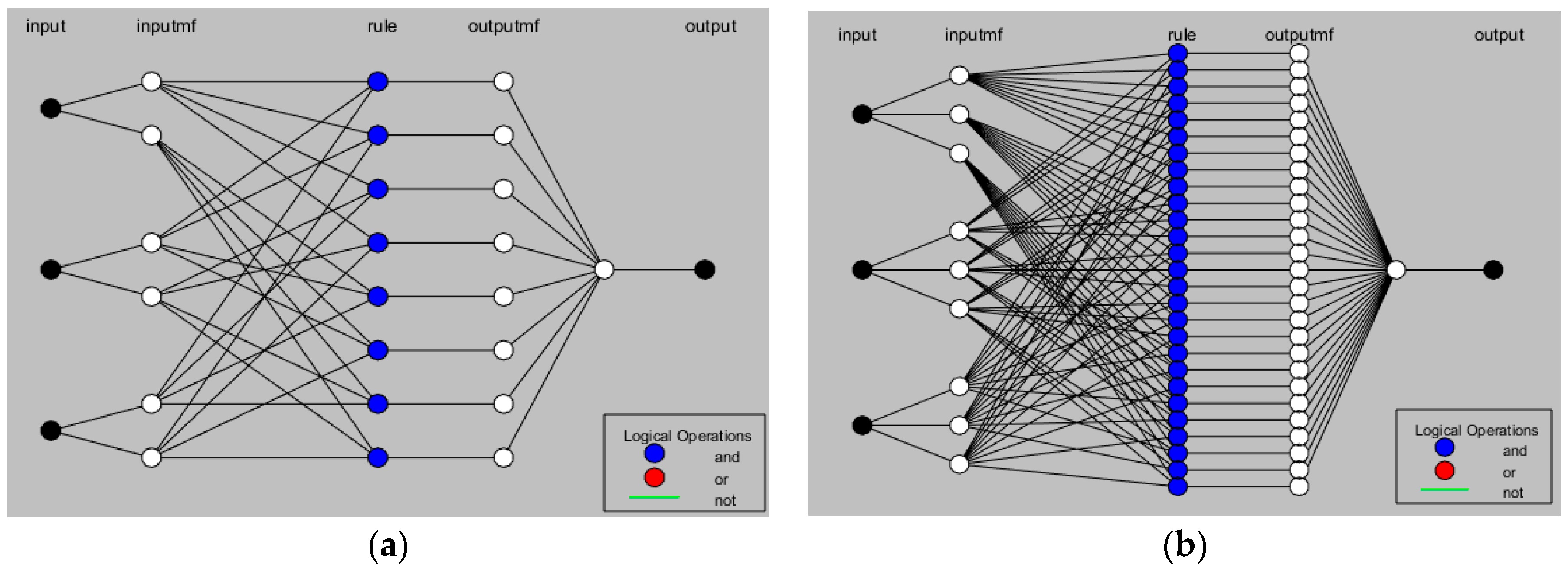
2.2. The Empirical Model—Adaptive Neuro-Fuzzy Inference System (ANFIS)

Adaptive neuro-fuzzy inference systems (ANFIS) belong to a family of hybrid systems. They use a supervised learning on the learning algorithm which has a function similar to the model of the Takagi–Sugeno fuzzy inference system [11]. An ANFIS combines the advantages of fuzzy logic (FL) and artificial neural networks (ANNs) for modeling purposes. ANNs operate in a black box manner and they have no capability of explaining a particular decision; on the other hand, ANNs have the ability to predict the output of a complex system through a learning process based on the examples provided [12,13]. FL itself possesses no learning ability but is able to provide mathematical descriptions in the form of linguistic terms and the structure of IF-THEN rules [14], offering an insight into decisions. An ANFIS can be used in a wide range of applications since it possesses the ability to handle large amounts of data in nonlinear and dynamic systems, especially when relationships between data are not fully understood.

Figure 4 shows the ANFIS scheme. The ANFIS structure consists of five connected network layers, $l_1$ to $l_5$. The first and fourth layers contain adaptive nodes while the other layers contain fixed nodes represented in circular shapes. The adaptive nodes contain parameters that are modified to achieve the desired input–output mapping, while the fixed nodes contain none. The architecture of the ANFIS is presented based on two fuzzy IF-THEN rules and the first order Sugeno model as follows:

• Rule 1: if $x$ is $A_1$ and $y$ is $B_1$, then $f_1=p_{1}x+q_{1}y+r_1$.
• Rule 2: if $x$ is $A_2$ and $y$ is $B_2$, then $f_2=p_{2}x+q_{2}y+r_2$.

where:

• $x$ and $y$ are the inputs,
• $A_i$ and $B_i$ are the membership functions (MF),
• $f_i$ is the output, and
• $p_i$, $q_i$ and $r_i$ are the linear design parameters (consequent parameters), determined during the training process [16].

In $l_1$ all nodes are adaptive nodes. Inputs are presented as $x$ and $y$. The output of a node is the membership value $O_{1,i}$, that specifies the degree of input $x$ (or $y$) belonging to fuzzy set $A_i$ (or $B_i$):

$$O_{1,i}={\mu }_{ A_i}\left(x\right),$$

(1)

$$O_{1,i}={\mu }_{B_{i-2}}\left(y\right),$$

(2)

we adopt the Gaussian MF by:

$${\mu }_{ A_i}\left(x\right)=exp\left[-{\left(\frac{x-a_i}{c_i}\right)}^2\right] ,$$

(3)

where $a_i$ and $c_i$ are the shape parameters (premise parameters) of an MF.

Layer $l_2$ is the rule layer with fixed or nonadaptive nodes labeled as $\pi$. As an output, it computes the firing strength $w_i$ (activation level) of each rule with the AND logical operator (or with other types of T-norm operators with general performance):

$$O_{2,i}=w_i={\mu }_{ A_i}\left(x\right)*{\mu }_{B_i}\left(y\right).$$

(4)

In $l_3$ is the normalization layer with fixed nodes, labeled as $N$. The outputs of this layer are normalized representations of each rule:

$$O_{3,i}=\overline{w_i}=\frac{w_i}{w_1+w_2}.$$

(5)

Layer $l_4$ contains adaptive nodes. The output of each node is the product of normalized firing strength and a first order polynomial (for a first order Sugeno model):

$$O_{4,i}=\overline{w_i}*f_i=\overline{w_i}*\left(p_{i}x+q_{i}y+r_i\right).$$

(6)

Layer $l_5$ contains a single fixed node, labeled as ${\displaystyle \sum }$. It computes the summation of all the input signals coming from the nodes in layer $l_4$:

$$O_{5,i}={{\displaystyle \sum }}_i\overline{w_i}*f_i=\frac{{{\displaystyle \sum }}_i{w}_i*f_i}{{{\displaystyle \sum }}_i{w}_i}.$$

(7)

Consequent and premise parameters are computed during the training process, based on the back-propagation gradient descent algorithm or with hybrid learning [15].

2.3. Particle Swarm Optimization

The particle swarm optimization algorithm (PSO) stochastic metaheuristic computational method was developed by Eberhart and Kennedy in 1995 [17]. PSO and other metaheuristic algorithms do not guarantee a global optimal solution, yet they have proven to be essential in near-optimal solution searches in vast nonlinear multidimensional solution spaces [18]. The algorithm mimics the intelligence of a flock of birds (swarm), based on the socio-psychological correlations [19] expressed by mathematical formulae over the bird’s (particle’s) position and velocity. The position of a particle represents a possible solution, while velocity can be described as the pulling tendency of a particle in the direction of the next solution search. PSO enables an iterative solution search by moving particles through the search space, trying to improve the candidate’s solution regarding the given fitness function representing a measure of quality. Fitness function represents how good the multidimensional position of an i-th particle is. Particles move according to their personal and global best positions. Conceptually, personal best ($pbes{t}_{id}$) imitates a particle’s autobiographical memory: it tends to push each particle to the place at which the current particle was most satisfied. Global best ($gbest$) is conceptually similar to a collective knowledge: it tends to pull all particles in the direction represented by the best position (achieved until now) of any particle in a swarm.

In the first iteration, particles’ positions are generated randomly as multidimensional constrained vectors, with initial velocities set to zero. Through the iteration process of the solution search, the particles’ velocities $v_{id}^t$ are altered with:

$$v_{id}^{t+1}=w{v}_{id}^t+C_{1}ran{d}_1*\left(pbes{t}_{id}-x_{id}^t\right)+C_{2}ran{d}_2*\left(gbest-x_{id}^t\right)$$

(8)

and positions $x_{id}^t$ with:

$$x_{id}^{t+1}=x_{id}^t+v_{id}^{t+1}.$$

(9)

where:

• $id$ subscript represents the current particle,
• $t$ is the current iteration,
• w is the inertia weight coefficient,
• $C_1$ and $C_2$ are the acceleration coefficients, and
• $ran{d}_1()$ and $ran{d}_2$() represent random number generators.

To control the system’s convergence tendencies, a set of restriction coefficients $w$, $C_1$ and $C_2$ was adopted, according to Kennedy and Clerc’s recommendations [20], that has proven to work sufficiently well on a variety of different optimization problems. The positions $x_{id}^t$ were represented as external ANFIS input parameters. The PSO algorithm was set to stop after a certain number of iterations.

2.4. Workflow and Validation

In this study, we presented two cases: case $1$ consisted of the ANFIS modeling and prediction of the temperature difference output. It started by dividing the dataset (input–output data points) into training and testing sets. The training set was used for the ANFIS model construction and the testing set for evaluating the ANFIS model on the data yet unseen by the model. In $\mathrm{k}$-fold cross-validation, the original dataset was randomly partitioned into $k$ equal sized sub partitions. The $k-1$ sub partitions were used as training data and a single partition was used for the testing of the ANFIS structure. During the cross-validation procedure, all external ANFIS input parameters, such as number of membership functions (MF), type of MF, number of epochs, learning step, increase in learning step and optimization method, were kept fixed. The whole cross-validation procedure was then repeated $k$ times, with each of the $k$ sub partitions used exactly once as testing data. In the majority of cases presented in this paper, the leave one subject out (LOSO) validation scheme ($k=35$) was adopted, partitioning the whole dataset into $35$ equal parts and performing $35$ iterations of learning with $34$ folds and testing on the remaining fold (yet every iteration a different fold). The LOSO procedure promised better overall generalization of the model’s performance and enabled the use of the whole dataset for both the model’s learning and its testing. The root mean squared error (RMSE) was used as a fitness function and represented the quantitative evaluation of the ANFIS’s performance.

Case $2$’s procedure was structurally the same as that of case $1$, except for an additional part represented by the PSO algorithm, which was set to optimize the external ANFIS input parameters. As the PSO fitness function, the RMSE testing error was adopted. The PSO algorithm was set to minimize the RMSE testing error and consequently find optimal ANFIS input parameter settings (Figure 5).

3. Results and Discussion

3.1. Case 1

During the ANFIS model’s formulation, the number of MFs for each input, type of MF, number of learning epochs, initial step size and step size increase rates were varied. In case 1, variations of different types of MF were used, such as generalized bell-shaped, triangular, trapezoidal, pi-shaped, Gaussian’s and Gaussian combination MF. The type of MF has not altered the results in a significant manner. Modeling with a different number of MFs for each input (dependent variable) was also performed. Increasing the number of MF number, computational time and number of IF-THEN rules formed by the ANFIS also increase. Input MFs were generated using the grid partition clustering method that uniformly partitioned the input variable ranges and created a single-output Sugeno fuzzy system. Other clustering methods, such as subtractive clustering, have achieved lower modeling precision rates. A Gaussian MF was adopted and the ANFIS structure (Figure 6) was trained for $100$ epochs using back-propagation and a hybrid algorithm to determine the premise and consequent parameters, with an initial step size equal to $0.1$. and a step size increase rate of $1.10$. Results are stated in Table 1 for the LOSO cross-validation. The ANFIS structure trained with three MF and the hybrid learning algorithm computed the lowest training RMSE (= 8.37 × 10⁻⁷) but a relatively high testing RMSE ($=0.8594$). Lowering the number of epochs did not result in improving the generalization ability of the discussed ANFIS that tended to overfit the training set.

The computational time of the ANFIS with back-propagation learning and two MFs achieved the best results with the input parameters stated in the above paragraph. The discussed ANFIS was about $5.6$ times faster compared to the ANFIS structure with the hybrid learning algorithm and three MFs, $4.8$. times faster than the ANFIS with back-propagation learning and three MFs and had a similar computation time to the ANFIS structure with hybrid learning and two MFs.

Based on the set of results in

Table 2. ANFIS information.

ANFIS Information
Learning method	hybrid	hybrid	Back-propagation	Back-propagation
Output MF	linear	linear	linear	linear
Number of MF per input	2	3	2	3
Number of nodes	34	78	34	78
Number of linear parameters	32	108	32	108
Number of nonlinear parameters	18	27	18	27
Number of fuzzy rules	8	27	8	27
Training RMSE	0.0603	8.37 × 10−7	0.1643	0.1769
Test RMSE	0.8125	0.8594	0.3450	0.5507
Training R2	0.9985	1.000	0.9855	0.9549
Test R2	0.6775	0.4051	0.6917	0.4870
Time (sec)	8.04	42.85	7.60	36.44

, further experiments (Figure 7) were performed on the ANFIS structure with the same ANFIS input parameters and back-propagation learning algorithm and two Gaussian MFs. To produce the results in Figure 7, the 10-fold cross-validation was used. Two Gaussian MFs were used due to their simplicity and high performance (low computation). In further experiments, six different initial step sizes ($0.001$, $0.005$, $0.01$, $0.05$, $0.1$ and $0.5$) and six different step size increase values ($1.00001$, $1.001$, $1.1$, $1.2$, $1.3$ and $1.4$) were used for the ANFIS model construction. The ANFIS structure with the $0.1$ initial step size and $1.001$ step size increase achieved the best test RMSE ($=0.4195$) as can be seen in Figure 7a. The train RMSE of the mentioned structure was $0.1254$ as depicted in Figure 7b.

3.2. Case 2

The particle swarm optimization algorithm (PSO) was used for the optimal external ANFIS input parameters search in the so called PSO-ANFIS procedure. Optimization was set to find the minimum testing RMSE based on the LOSO cross-validation procedure by altering the initial step size (ISS) and step size increase (SSI) via PSO. ANFIS input parameters such as number of MFs, type of MF and number of epochs were kept fixed (two Gaussian MFs, trained for $100$ epochs with the back-propagation learning algorithm). The ANFIS structure was trained based on the back-propagation learning algorithm to determine the premise and consequent parameters.

One hundred PSO particles were used in the optimum search. PSO was set to work for $100$ iterations, with a set of restriction coefficients $w=0.729$, $C_1=1.496$ and $C_2=1.496$. Each PSO particle’s fitness function value was calculated with LOSO: in our case, this was $35$-fold cross-validation. The convergence of the PSO algorithm is shown in Figure 8. The initial positions of the PSO particles, represented by ISS and SSI, were created with a random number generator at intervals of ($0$,$10$) and (1,$10$), respectively. Case $2$, consisting of the ANFIS model and the PSO module, proved to achieve similar optimum values in multiple runs with different initial positions for the ISS and SSI. Additional external parameters, such as iteration number, number of MFs or step size decrease rate could be introduced in a similar manner to ISS and SSI.

This section presents an analysis of the results of the experimental data and the ANFIS model output on the nitrogen cooling impact during the machining of Inconel $718$.

Table 3. Experiment inputs, outputs and predicted output (based on the testing set) of optimized ANFIS and percentage difference between outputs.

$\mathit{v}$ [m/min]	$\mathit{d}$ [mm]	$\mathit{x}$ [mm]	$\mathbf{\Delta }\mathit{T} \left[\mathbf{K}\right]$	$\mathbf{\Delta }{\mathit{T}}_{\mathit{c}\mathit{a}\mathit{s}\mathit{e}1} \left[\mathbf{K}\right]$	$\mathbf{\Delta }{\mathit{T}}_{\mathit{c}\mathit{a}\mathit{s}\mathit{e}2 \mathit{b}\mathit{e}\mathit{s}\mathit{t}} \left[\mathbf{K}\right]$
5	0.1	5	3.2517	2.2990	2.7937
		10	2.3180	2.6407	2.4037
	0.5	0	5.7544	3.1399	3.2125
		5	2.2840	3.0916	3.1094
		10	1.8445	1.9927	1.3562
	1	0	3.3258	2.2173	1.9850
		5	1.9913	1.5084	2.1284
		10	1.4317	1.0998	1.4480
15	0.1	0	1.9796	2.2419	2.1050
		5	1.2245	0.9262	1.0530
		10	0.9354	0.6331	1.0758
	0.5	0	2.1012	1.9184	2.3156
		5	0.8687	1.3459	1.1354
		10	0.7829	0.6331	0.8089
	1	0	0.0872	0.0352	0.1320
		5	0.0754	0.0227	0.0314
		10	0.0485	0.0617	0.0547
25	0.1	0	1.3235	1.2691	1.4158
		5	0.8455	0.1928	0.8042
		10	0.5057	0.4781	0.5750
	0.5	0	1.2517	1.0434	1.3065
		5	1.1352	0.5572	0.6713
		10	0.3763	0.7014	0.6201
	1	0	0.0687	0.1075	0.0682
		5	0.1148	0.1483	0.2113
		10	0.1193	0.1975	0.2759
35	0.1	0	0.3686	0.1927	0.3734
		5	0.2779	0.5793	0.4713
		10	0.3592	0.2636	0.3178
	0.5	0	0.2790	0.4457	0.4316
		5	0.3057	0.4535	0.5660
		10	0.3448	0.1845	0.3113
	1	0	0.2546	0.1296	0.2175
		5	0.2446	0.3129	0.3007
		10	0.3993	0.1667	0.2239

and Figure 9 represent the predicted temperature differences of the ANFIS structures compared to the real experiment values. The first three columns in Table 3 present the experimental values ($v$, $d$ and $x$), the fourth column the experimental value ($\mathsf{\Delta }\mathrm{T}$) and the fifth column the temperature difference (${\mathsf{\Delta }\mathrm{T}}_{\mathrm{case}1}$) of the testing set predicted in case $1$ based on the LOSO cross-validation. The sixth column represents the temperature differences (${\mathsf{\Delta }\mathrm{T}}_{\mathrm{case}2 \mathrm{best}}$) of the testing set predicted in case $2$. The optimized ANFIS structure in case 2 with $ISS=1.6764$ and $SSI=7.7766$ achieved the testing RMSE equal to $0.2620$ and a training RMSE of $0.3372$. The respective testing and training R² values were equal to $0.8585$ and $0.8912$.

The average difference between the experimentally measured temperature drop ($\mathsf{\Delta }\mathrm{T}$) and the temperature drop predicted by the ANFIS based on the LOSO testing set in case $1$ ($\left|\mathsf{\Delta }\mathrm{T}-{\mathsf{\Delta }\mathrm{T}}_{\mathrm{case}1}\right|$) was equal to $0.3450$ °C, while the optimized ANFIS structure in case $2$ achieved an average temperature difference between the experimentally measured temperature drop ($\mathsf{\Delta }\mathrm{T}$) and the temperature drop predicted by ANFIS based on the LOSO testing set ($\left|\mathsf{\Delta }\mathrm{T}-{\mathsf{\Delta }\mathrm{T}}_{\mathrm{case}2 \mathrm{best}}\right|$) equal to $0.2619$ °C.

Neural networks combined with fuzzy logic in the ANFIS system offer an insight into their decisions. Figure 10 presents the Fuzzy interference system (FIS) properties of the discussed ANFIS. Output ($\Delta T$ represented by a first order Sugeno model) was calculated based on eight IF-THEN rules that represent all combinations of input MFs ($=2^3$). The premise parameters are stated as $a_i$ and $c_i$, where $a$ represents the mean and $c$ the width of the $i$-th Gaussian MF. The first rule states that if the input 1 belongs to MF1, input $2$ to MF3 and input 3 to MF5, then output is determined by $\Delta T=m_1*input1+p_1*input2+q_1*input3+r_1$. The consequent parameters of the $1$-st rule, denoted as $m_1$, $p_1$, $q_1$ and $r_1$, are equal to $-0.5706$, $-0.1155$, $-0.0434$ and $8.896$, respectively.

4. Conclusions

In the past decade, sustainable machining has become increasingly important. The use of an alternative cooling lubrication fluid which is not harmful to the environment and human health is encouraged. Nowadays, cryogenic machining sets sustainable trends in machining technologies, which represents guidelines for the implementation of sustainable technologies in production, where the use of harmful cooling lubrication is reduced. The modern guidelines of machining emphasize the consumption of cooling lubrication fluids which do not affect human health and the environment. As part of these trends, the idea of sustainable development at all levels of life has emerged. This paper explains the aspects of the use of liquefied nitrogen as a cooling medium in cryogenic machining and thus contributes to basic knowledge in the field of cooling effects, promising greater involvement and promotion of sustainable engineering in the industry. The objective of this research was to analyze the thermal influence of liquefied nitrogen on workpieces depending on variation of the input parameters to obtain correlation with the measured temperature.

The effect of the conductance of liquefied nitrogen on workpieces was reduced due to the formation of a gaseous film which had very low thermal conductivity cca. 0.03 W/mK and a low heat transfer coefficient in comparison to the liquid nitrogen phase. The nozzle must be placed as close as possible to the cutting zone to ensure the most efficient cooling capacity of the medium and thus the smallest possible dissipation of the jet.

To predict temperature drops in the material, various versions of ANFIS models were applied to predict the temperature difference of Inconel $718$ cooling with liquefied nitrogen. Various ANFIS model configurations were proposed and discussed. The ANFIS model (case 1) and the ANFIS structure combined with PSO (case $2$) were proven to achieve low modeling errors of the temperature drops in Inconel 718. The best values of RMSE achieved were low, stating the ANFIS’s modeling ability of liquefied nitrogen cooling. Since the study was conducted with a small number of experiments (input–output datapoints), the LOSO k-fold cross-validation procedure was adopted, enabling the more representative accuracy of the presented ANFIS models, which were not suited to fixed and/or small sets of datapoints. LOSO offered to exploit the small datasets and by them assess the overall ANFIS modeling performance. Depending on the nature of the problem, additional external ANFIS input parameters (not only ISS and SSI) can be included. Including additional external input parameters prolongs the computation time, which is still shorter compared to other hybrid approaches since fewer independent variables are included.

References

1. Pusavec, F.; Courbon, C.; Rech, J.; Kopac, J.; Jawahir, I. Importance of the Nitrogen Phase on the Cryogenic Machining Performance. In Proceedings of the ASME International Manufacturing Science and Engineering Conference, Detroit, MI, USA, 9–13 June 2014. [Google Scholar]
2. Pusavec, F.; Hamdi, H.; Kopac, J.; Jawahir, I.S. Surface integrity in cryogenic machining of nickel based Alloy—Inconel 718. J. Mater. Process. Technol. 2011, 211, 773–783. [Google Scholar] [CrossRef]
3. Pusavec, F.; Deshpande, A.; Yang, S.; M′Saoubi, R.; Kopac, J.; Dillon, O.J.; Jawahir, I. Sustainable machining of high temperature Nickel Alloy—Inconel 718: Part 1—Predictive Performance Models. J. Clean. Prod. 2014, 81, 255–269. [Google Scholar] [CrossRef]
4. Yildiz, Y.; Nalbant, M. A Review of Cryogenic Cooling in Machining Processes. Int. J. Mach. Tools Manuf. 2008, 48, 947–964. [Google Scholar] [CrossRef]
5. Mozammel, M.; Dhar, N.R. Response surface and neural network based predictive models of cutting temperature in hard turning. J. Adv. Res. 2016, 7, 1035–1044. [Google Scholar]
6. Chinchanikar, S.; Choudhury, S. Machining of hardened steel—Experimental investigations, performance modeling and cooling techniques: A review. J. Mach. Tools Manuf. 2015, 89, 95–109. [Google Scholar] [CrossRef]
7. Ezugwu, E.O.; Fadare, D.A.; Bonney, J.; Da Silva, R.B.; Sales, W.F. Modelling the correlation between cutting and process parameters in high-speed machining of Inconel 718 Alloy using an artificial neural network. Int. J. Mach. Tools Manuf. 2005, 45, 1375–1385. [Google Scholar] [CrossRef]
8. Elbaz, K.; Shen, S.-L.; Zhou, A.; Yuan, D.-J.; Xu, Y.-S. Optimization of EPB shield performance with adaptive neuro-fuzzy inference system and genetic algorithm. Appl. Sci. 2019, 9, 780. [Google Scholar] [CrossRef] [Green Version]
9. Elbaz, K.; Shen, S.-L.; Yin, Z.; Zhou, A. Prediction Model of shield performance during tunneling with AI via incorporating improved PSO into ANFIS. IEEE Access 2020, 8, 39659–39671. [Google Scholar] [CrossRef]
10. Hriberšek, M.; Šajn, V.; Pušavec, F.; Rech, J.; Kopac, J. The procedure of solving the inverse problem for determining surface heat transfer coefficient between liquified Nitrogen and Inconel 718 Workpiece in Cryogenic Machining. J. Mech. Eng. 2016, 62, 331–339. [Google Scholar] [CrossRef]
11. Suparta, W.; Alhasa, K.M. Modeling of Tropospheric Delays Using ANFIS; Cham Springer International Publishing: Cham, Switzerland, 2016. [Google Scholar]
12. Simeunovic, N.; Kamenko, I.; Bugarski, V.; Jovanovic, M.; Lalic, B. Improving workforce scheduling using artificial neural networks model. APEM J. 2017, 12, 337–352. [Google Scholar] [CrossRef]
13. Klancnik, S.; Begic-Hajdarevic, D.; Paulic, M.; Ficko, M.; Cekic, A.; Cohodar, M. Prediction of laser cut quality for Tungsten Alloy. Using the neural network method. J. Mech. Eng. 2015, 61, 714–720. [Google Scholar]
14. Senthilkumar, N.; Sudha, J.; Muthukumar, V. A grey-fuzzy approach for optimizing machining parameters and the approach angle in turning AISI 1045 Steel. APEM J. 2015, 10, 195–208. [Google Scholar] [CrossRef]
15. Jang, J.-R. ANFIS: Adaptive-Network-Based Fuzzy Inference System. IEEE Trans. Syst. Man Cybern. 1993, 23, 665–685. [Google Scholar] [CrossRef]
16. Al-Hmouz, A.; Shen, J.; Al-Hmouz, R.; Yan, J. Modeling and simulation of an adaptive neuro-fuzzy inference system (ANFIS) for mobile learning. IEEE Educ. Soc. 2011, 5, 226–237. [Google Scholar] [CrossRef]
17. Kennedy, J.; Eberhart, R. Particle Swarm Optimization. In Proceedings of the ICNN’95—International Conference on Neural Networks, Perth, Australia, 27 November–1 December 1995; Volume 4, pp. 1942–1948. [Google Scholar]
18. Cheng, Q.; Zhan, C.; Liu, Z.; Zhao, Y.; Gu, P. Sensitivity-based multidisciplinary optimal design of a hydrostatic rotary table with particle swarm optimization. J. Mech. Eng. 2015, 61, 432–447. [Google Scholar] [CrossRef]
19. Hrelja, M.; Klancnik, S.; Irgolic, T.; Paulic, M.; Balic, J.; Brezocnik, M. Turning Parameters Optimization Using Particle Swarm Optimization. In Proceedings of the 24th DAAAM International Symposium on Intelligent Manufacturing and Automation, Zadar, Croatia, 23–26 October 2013; Volume 69, pp. 670–677. [Google Scholar]
20. Clerc, M.; Kennedy, J.; Kennedy, J. The Particle Swarm—Explosion, stability and convergence in a multi-dimensional complex space. IEEE Trans. Evol. Comput. 2002, 6, 58–73. [Google Scholar] [CrossRef] [Green Version]
Figure 1. Schematic illustration of the moving nozzle with corresponding positions of the thermocouples and a cross section view of the holes at different depths [10].
Applsci 10 03603 g001
Figure 2. Experimental setup [10].
Applsci 10 03603 g002
Figure 3. The example of temperature–time distribution curve Texp(t) for Inconel 718 and time of the nozzle moving across the plate (v = 5 m/min and d = 0.5 mm) [10].
Applsci 10 03603 g003
Figure 4. The adaptive neuro-fuzzy inference system (ANFIS) architecture [15].
Applsci 10 03603 g004
Figure 5. Case 1 and case 2 flowchart representations.
Applsci 10 03603 g005
Figure 6. ANFIS network with two membership functions (MFs) (a) and three MFs (b).
Applsci 10 03603 g006
Figure 7. ANFIS model train (a) and test RMSE accuracies (b). Structures were trained with back-propagation for 100 epochs, two Gaussian MFs per input, different initial step sizes and different step size increase rates.
Applsci 10 03603 g007
Figure 8. Convergence of the solution. ISS stands for initial step size, SSI for step size increase and FF for fitness function represented by the testing RMSE.
Applsci 10 03603 g008
Figure 9. Column bar chart representing the temperature differences between experimental values Δ T (blue bars), predicted PSO-ANFIS Δ T c a s e 2   b e s t (orange bars) and ANFIS Δ T c a s e 1 (gray bars).
Applsci 10 03603 g009
Figure 10. FIS properties of optimized ANFIS (case 2), with all 35 measurements used for training.
Applsci 10 03603 g010