Groundwater Level Fluctuation Analysis in a Semi-Urban Area Using Statistical Methods and Data Mining Techniques—A Case Study in Wrocław, Poland

Abstract

Long-term groundwater level analysis, which is usually based on traditionally defined hydrological years is essential in an era of global warming and other climatic and environmental changes, especially in urban areas. A complex interplay of multiple factors influencing the groundwater level makes the investigation of their interdependencies a challenge. Based on multiple data sets and a long time series available as well as specific geological and hydrological conditions, a semi-urban district of Wrocław/Poland was selected as a case study for investigating these dependencies. This paper presents an interdisciplinary approach to the analysis of groundwater level fluctuations by combining mathematics, signal processing, hydrogeology, and meteorology. Applying well-known methods from disciplines other than hydrogeology, the authors investigated seasonal behavior and similarity of groundwater level fluctuations during 15 hydrological years. Based on segmentation and agglomerative clustering (AHP), five classes of groundwater levels fluctuations for predefined hydrologic years and the corresponding seasons were identified and compared to the classification scheme by Pleczyński. Additionally, the relationship between precipitation and groundwater level was investigated using Pearson, Kendall and Spearman correlations. This led to the identification of “typical” and “untypical” seasons for the correlation between the cumulative precipitation sum and groundwater levels. The results presented here will be used for further investigations of groundwater level fluctuations using additional factors and statistical methods. These aim to identify periods that describe similarities better than the commonly used hydrological year.

1. Introduction

Groundwater, amounting to 23.4 million km${}^3$, is the second largest resource of freshwater in the world, after glaciers and permanent ice caps with a volume of 32.9 million km${}^3$, and the only widely accessible fresh water source [1,2,3]. In the time of global water scarcity, groundwater is under high stress, especially in urban and semi-urban areas where not only global warming influences its quantity, but also many artificial factors have a negative effect on the available volume of groundwater [4]. To manage this precious resource properly, we have to know how much water exists in the aquifer. For that, we need long-term groundwater level observations, which are important for effective and sustainable water management, geoengineering as well as for a reliable freshwater supply. Based on the data gathered during the observation period we can define and describe natural and artificial factors influencing groundwater levels resulting in water resource quantity estimations and predictions. As longer observation periods are favorable for reliable statistical analysis and predictions in Earth sciences, we used the longest time series accessible to us in Wrocław, Poland.

Groundwater level fluctuations are indicative for changes in the quantity of water stored underground. Mid and long term analysis of groundwater level fluctuations refer to a specific cycle called water year or hydrological year (HY). It is the annual cycle that is associated with the natural progression of the hydrological seasons and depends on climate conditions and differs in different regions of the world (in Poland its duration is from 1 November until 31 October).

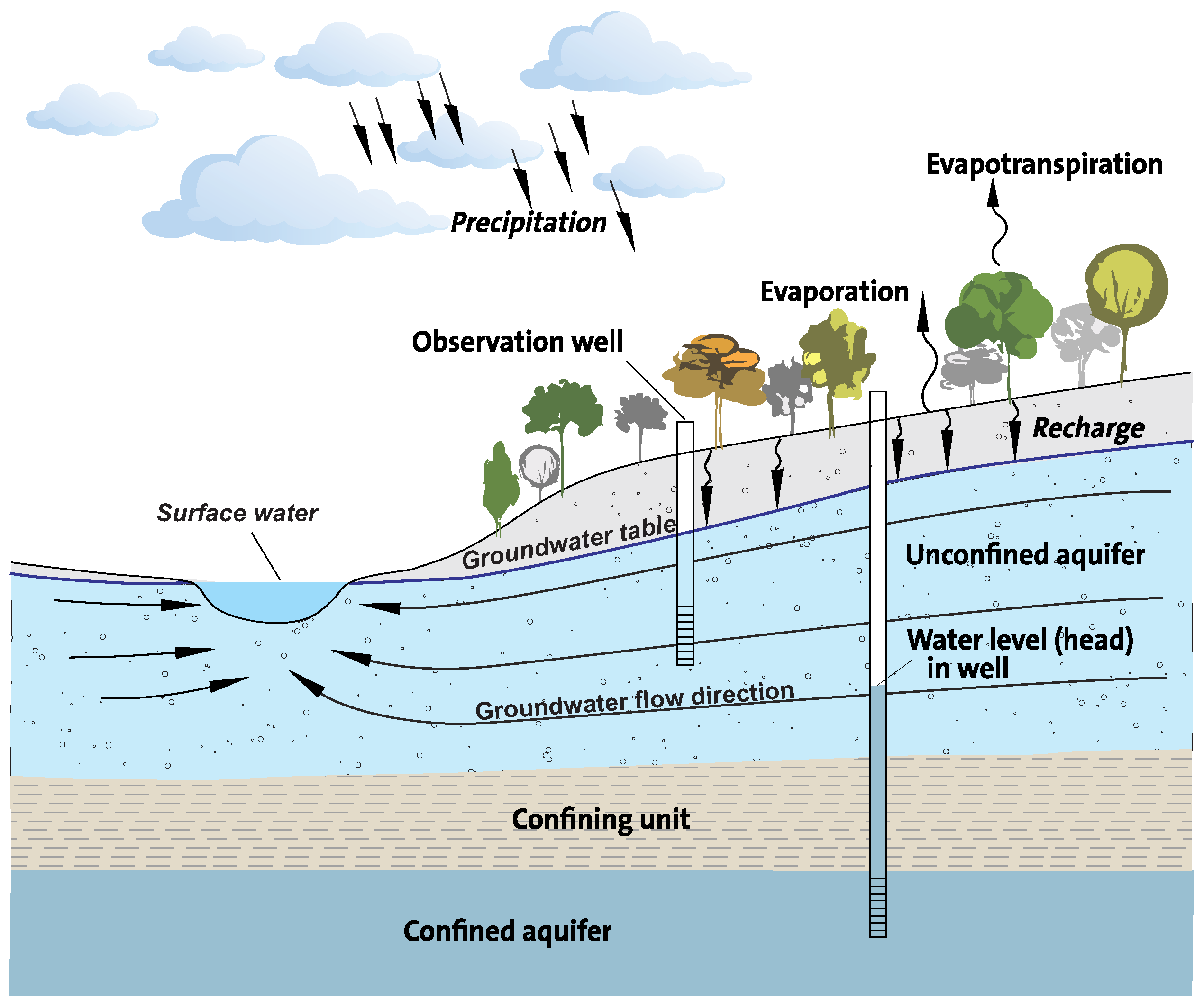
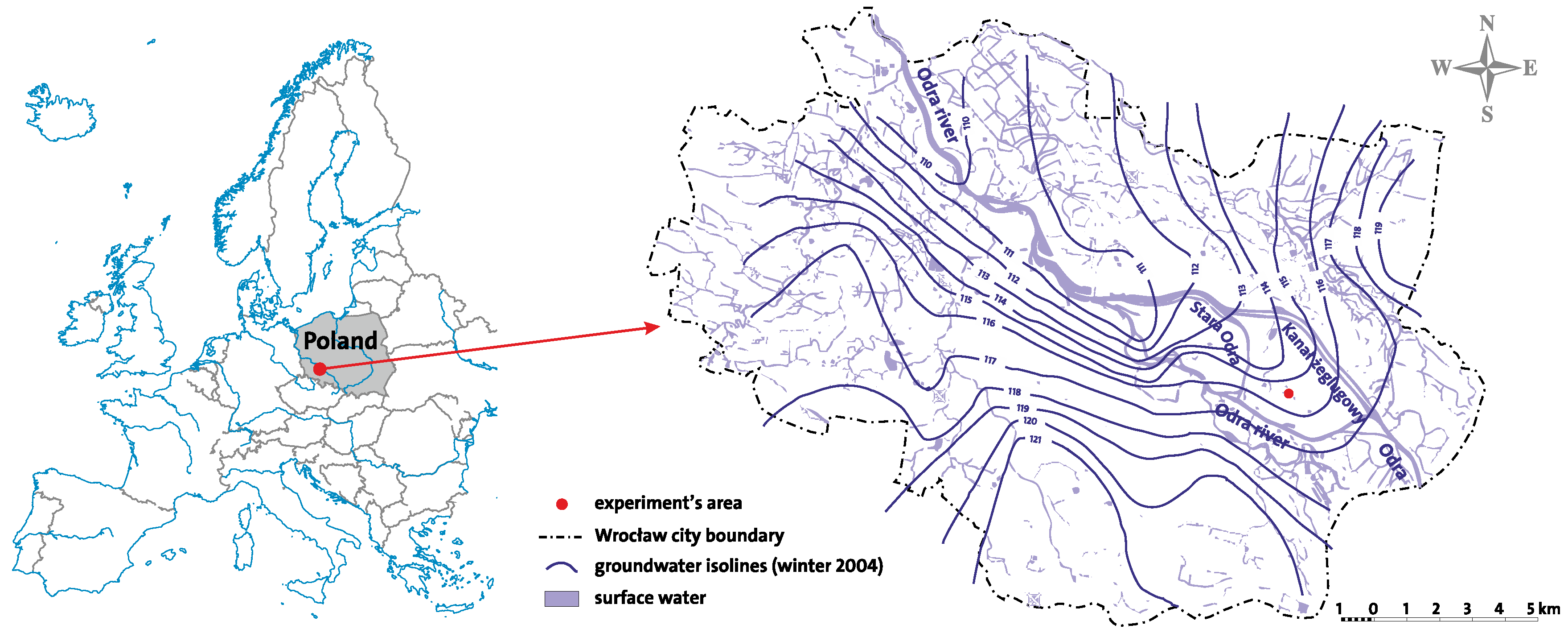
Groundwater level fluctuations in undisturbed conditions depend on the geological setting and the permeability of the unsaturated (vadose) zone as well as on precipitation, air temperature, air moisture and insolation (Figure 1). These factors can be easily measured with sensitive automated sensors nowadays. In urban and semi-urban areas, there are many unmeasurable factors influencing the groundwater level that can disturb its seasonal (cyclic) nature (e.g., regulated water streams, surface pavements, drainage). By combining mathematics, signal processing, hydrogeology, and meteorology, some new opportunities for long-term analysis of groundwater fluctuation can be derived. There are key questions to be answered: (i) does the groundwater level in a semi-urban area behave in a similar way every hydrological year and season? (ii) is the predefined duration of the hydrogeological year still valid in this semi-urban area? and (iii) are there any anomalies in the groundwater level fluctuations and what are the reasons for that? Thus, to develop a model for anomaly detection and future prediction of relationships between groundwater level, precipitation and temperature seems to be imperative. However, a precise relationship is unknown and also depends on the specific properties of a given area semi-urban part of a large city. This paper is an introduction to this kind of complex analysis and introduces methods well known from other applications that can be implemented for the groundwater level. Based on the example of one observation well in the city of Wrocław, data, first observations, preliminary analysis, and conclusions are presented. Reasons for choosing this single observation well are that it’s the city’s well with the longest nearly uninterrupted observation period, its location within the semi-urban area of Wrocław (Figure 2 and Figure 3), and the fact that the methods described had to be tested and evaluated first, before including additional wells with long term observations.

2. Current Situation

Groundwater level measurements have a long history, but one of the first cities which can boast off a complex analysis of its hydrogeological conditions is the city of Wrocław (Breslau). In 1876, the groundwater level in the city has been characterized for the first time by Jacobi [6]. He introduced general statistics of the groundwater level based on irregular measurements in few boreholes. Later, a network of 43 observation wells has been established by the City Council and regular measurements have been running by firefighters until 1922. All the results have been published in the statistical yearbooks ’Breslauer Statistik’. After this period only irregular and short-term observations in the city were conducted [7].

The importance of groundwater level observations has been emphasized by several studies in Germany and Austria since the end of the 19th century, but a more recent one in English language after Jacobi’s analysis is from Taylor and Alley [5]. They have explained basic rules of groundwater level monitoring and present case studies to highlight the wide range of applicability of long-term groundwater level data to varied water issues related to geoengineering or water management.

Groundwater monitoring data analysis has for decades been based on simple statistical methods [8]. Groundwater level prognosis had been primarily developed based on analytical methods and physical models [9]. In the 1990ies, numerical modeling with the implementation of the finite element method (FEM) or finite difference method (FDM) became common in predictions of groundwater conditions [10] as well as in predicting groundwater level and spatio-temporal analyses of climatic factors [11,12,13]. The last 15 years have also brought rapid development of other methods in research on Earth’s water system trends and on a description of groundwater level fluctuations phenomena. Implementation of wavelet analysis to evaluate factors controlling groundwater level fluctuations in a riverside alluvial aquifer was done by Oh et al. [14]. Combination of wavelets and neural networks has been used to forecast groundwater levels [15]. Groundwater level time series analysis and its relationships to different factors such as precipitation had also been studied using fractals [16,17,18]. There are also many works based on the implementation of different types of neural networks to groundwater analysis [19], as well as autoregressive models and advanced statistical methods for groundwater levels characteristics and predictions [20,21,22,23] including robust detrended analysis [24]. Groundwater potential mapping in the Dak Lak Province, Vietnam, implementing soft computing methods combined with advanced algorithms has been done by Nguyen et al. [25]. We can easily find the interconnection of cited research with methods applied to the analysis of other environmental processes [26]. One may notice universal problems as validation [27], segmentation [28,29], regime change [28,30], denoising [31], modelling [32] or processes separation [33] with using pattern extraction [28,33,34]. Often such analysis is performed in a multidimensional data space [30], where the problem of transformation to a specific domain or simple selection of informative features in multidimensional data space is needed [35]. There are some papers presenting the mentioned methods that are used for the analysis of groundwater issues [36,37,38,39,40,41], but they are not specifically focusing on groundwater level analysis but on the hydrogeochemistry or clustering the observation points. One of those studies [42] used Singular Value Decomposition (SVD) and a Cross-Wavelet Approach (CWA) to analyze the spatiotemporal groundwater level—precipitation relationship of 50 wells. The authors identified four time response lags and pointed out the importance of complete time series, especially of the precipitation near the wells. Lorentz et al. [43] found that the scale of the investigation is relevant for choosing the appropriate analytical technique for the recharge estimation. Depending on the scale, vertical or horizontal flow might be the relevant factor influencing the groundwater level. For accurate investigations, Hiscock and Bense [44] pointed out the importance of the barometric pressure and tidal effects on the groundwater levels.

Despite the fact that groundwater level fluctuation and groundwater data time series analysis are commonly used in modern research, there is a lack of study on the complex nature of the groundwater system in urban areas. This paper will investigate this phenomenon in more detail.

3. Experiment and Data Description

The city of Wrocław has characteristic geological, hydrogeological and hydrological conditions [45,46]. Inhabited by nearly 650 thousand people, the city is one of the largest in Poland [47]. Its history is over 1000 years long and is closely connected to the hydrography of the city. Located on the river Odra with its many branches, tributaries and channels, this forms a unique system with groundwater aquifers and renders the water issues in the city very important. Geologically, Wrocław is situated at the Middle Odra Fault Zone in the SW peripheral part of Fore-Sudetic Monocline, close to its border with the Fore-Sudetic Block. Its deep foundation is represented by Permian sandstones, conglomerates, anhydrite and limestone. Overlaying Triassic sandstones, limestone and marls are covered mostly by Miocene, Pliocene and Quaternary sediments [48]. Taking into account the 0–50 m thick Quaternary cover of Wrocław, two types of geological conditions can be distinguished [49]: a moraine upland, covering generally the SW and NE parts of the city and Odra valley deposits which cover the central part of the city and a 100–2000 m wide belt running in a NW–SE direction. While the moraine upland is dominated by clayey moraine and fluvioglacial sands and gravels, the Holocene Odra valley fills are composed of fluvial sands, gravel and silts of flood terraces and palaeo-river beds (Figure 4). Typically, the moraine upland clays have a thickness of 3–5 m, and within the city’s reach they are discontinuous, allowing the underlying Pliocene loams to surface. Groundwater levels in this part of the city are usually below 2 m. With a thickness of 20–50 m, the Holocene valley fills surpass the moraines’ thickness by far and the groundwater level of these permeable sediments is usually between 0 and 2 m deep.

Long-term observations of meteorological data, as well as groundwater levels, are run by the Observatory of the Department of Climatology and Atmospheric Protection at the University of Wrocław since 1946. The observatory field is situated in the semi-urban part of the city, on an island surrounded by the river Odra branches (Figure 2).

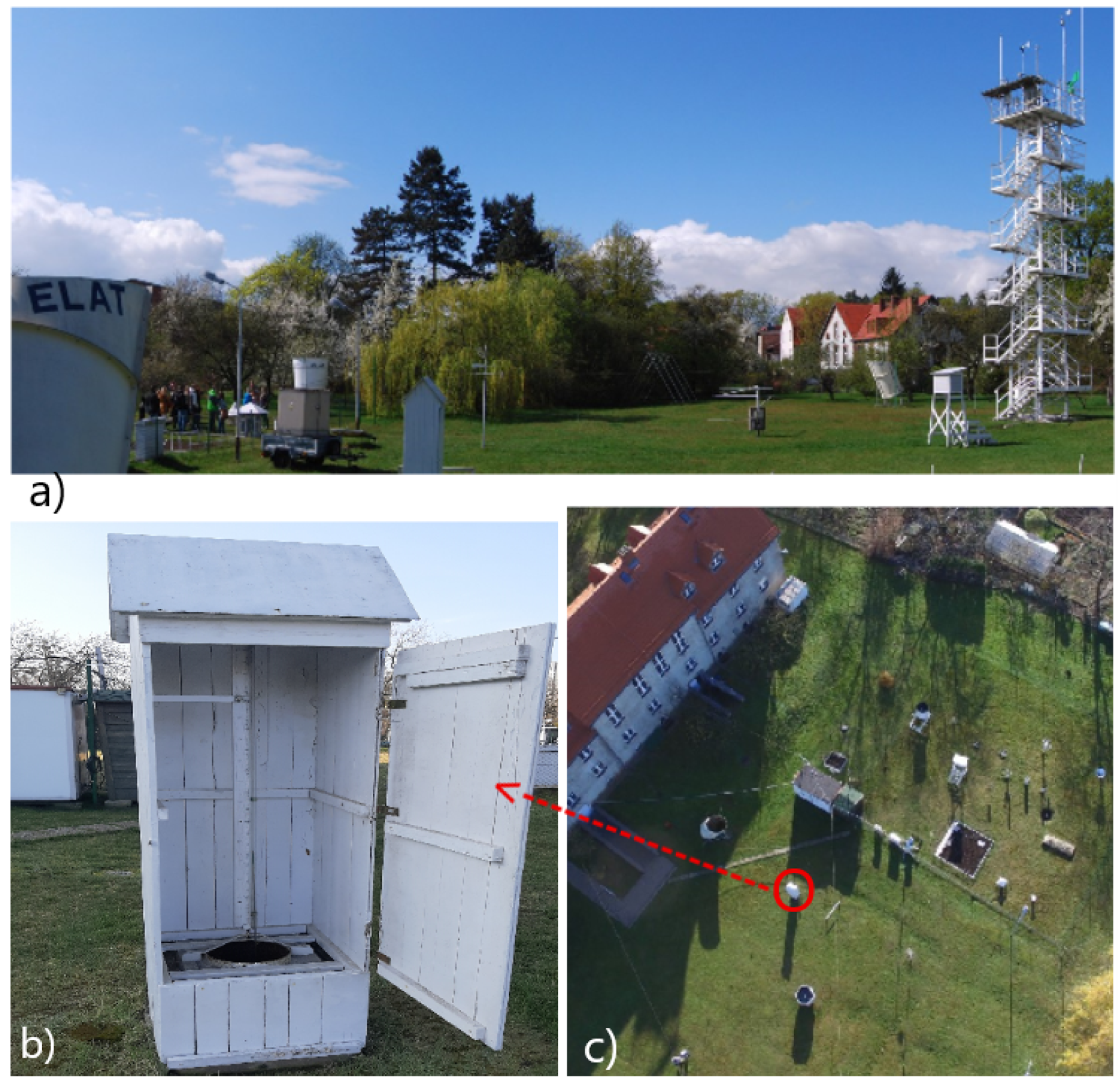
In this ‘garden-lab’, various data characterizing weather conditions, air quality and groundwater are collected daily. The observatory provided us with data on groundwater level, precipitation, air pressure, air temperature, air humidity and insolation data that have been gathered between 2003 and 2018, covering 15 hydrological years (Figure 5).

The groundwater level was measured in a 2.26 m deep piezometer located next to the other measuring devices in the observatory’s garden-lab with a float-meter installed in the borehole (Figure 3). The frequency of measurements was daily, with a gap between the 1 June 2014 and 3 July 2014 caused by a technical problem. That resulted in $n=5779$ samples with a vertical accuracy of 1 cm.

In the area of the monitoring well, the stratigraphy is dominated by sand and silty sand deposited during Holocene floodings of the river Odra (Figure 4). This sand can sometimes be coarse and it usually has a good hydraulic conductivity (1.7–2.6 × 10${}^{-3}$ cm/s [50]). Because the water level in the well ranges only between 1.2 and 2.2 m below the surface within these highly permeable sands, differences in the infiltration path length within the vadose zone were not taken into account for this study.

In parallel to the groundwater level, also the precipitation (R) was monitored using a Hellmann lowland rain gauge. The upper edge of the rain gauge is located 1 m above ground, and the area of the gauge-hole is 200 cm${}^2$. The precipitation was measured daily at 6 UTC, using a graduated scale in mm of the water column that resulted in $n=5844$ samples with an accuracy of 1 mm (Figure 5b). The sum of precipitation was measured for the previous day. In addition, the other factors that in theory could indirectly influence the groundwater levels were measured: the air temperature (T) and humidity (U). Their measurements are made using a Vaisala HMP45AC probe, equipped with a PT 100 temperature sensor with a measuring range of –40 ${}^{\circ }\mathrm{C}$ to +60 ${}^{\circ }\mathrm{C}$ and a Humica-p sensor for measuring relative humidity. The measurement of air temperature and relative humidity is carried out at a frequency of 1 min (Figure 5c,d) with gaps from 31 July 2008 to 10 September 2008, from 31 May 2012 to 7 January 2013, and from 31 August 2017 to 1 May 2018 in temperature and in the same time in humidity.

The two additionally measured parameters potentially influencing the groundwater level are the atmospheric pressure and total insolation. Atmospheric pressure was measured using a Vaisala PTA 427 barometer placed in a measuring container at the meteorological garden. The measurement is carried out in analogue to the air temperature every 1 min. The total insolation was measured with a Kipp&Zonen CMP3 pyranometer in W/m${}^2$, and it is placed on the actinometric tower, 15 m above ground level. In the investigated period, there have been gaps in the pressure data from 31 July 2008 to 10 September 2008 and from 31 May 2012 to 7 January 2013 (Figure 5) and in the insolation data from 31 July 2008 to 10 September 2008, from 31 July 2012 to 10 September 2012, and from 31 July 2016 to 5 September 2016 (Figure 5e,f). All the data gaps were caused by technical issues. From a mathematical point of view, the preliminary, visual analysis of the gathered data reveals interesting properties of the signals such as trend, periodicity, number of outliers and missing data. The images of each signal are different (Figure 5), which results in different analytical methodologies that need to be applied.

The nature of the groundwater level fluctuation is very complex and it is a function of the presented factors together with other data unavailable at this time, e.g., surface water levels or urban drainage [51]. That requires applying the advanced mathematical and statistical methods to their analysis.

4. Methods and Preliminary Analysis

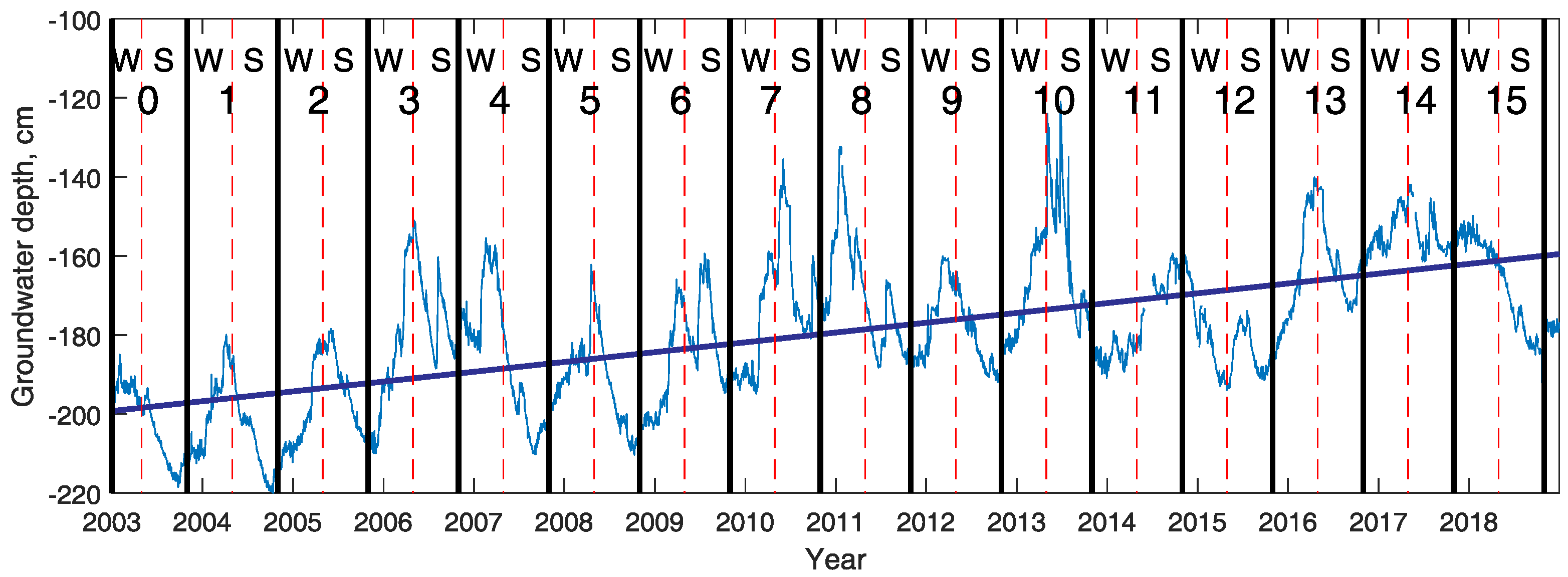
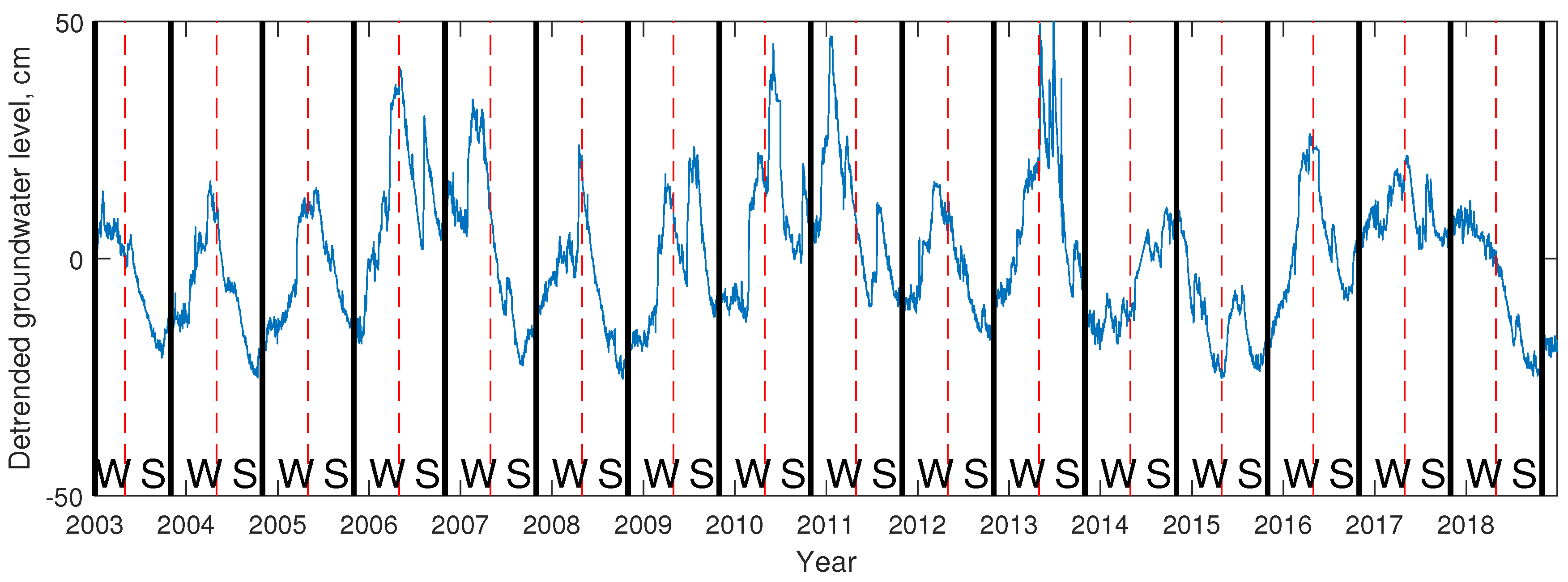
Analysis of real data usually comes with a number of challenges. Especially in Earth science, automatic data analysis should be preceded by careful validation of the raw data (e.g., missing data, disturbances, overdrive, interference, range of data). Any additional knowledge about the assumed behavior (e.g., seasonal, cyclic, random, deterministic) is valuable. The necessary part of the analysis and its results require a deep knowledge not only in mathematics and signal processing, but most of all in the specific field of Earth science. In this case, hydrogeology and meteorology are these two specific fields. The key challenge in this paper is to analyze signals related to groundwater level. The first task is related to the hydrological year (HY) self-similarity. Therefore, the signal has been segmented according to commonly accepted dates (black lines), and the winter and summer seasons have been marked in red (Figure 6).

A key question relates the similarity of consecutive hydrological years in the investigated period. It can clearly be seen that in each consecutive year, the patterns of the groundwater level fluctuations differ from the previous year and that the time series of the groundwater levels for some HYs is similar and for some is substantially different (Figure 6).

As also can be seen (Figure 6), the groundwater level data show a positive linear trend. Consequently, the next step was a detrending operation, which is commonly used as a preprocessing step, especially when looking for similarities between segmented data. In order to remove the trend, a linear dependence was identified and then subtracted from the whole time series of the groundwater level. If we denote the time series of the groundwater level as ${\{y_t\}}_{t=1}^m$ (m-total number of observations), then the linear trend is defined by the following formula:

$${\widehat{y}}_t=\widehat{a}t+\widehat{b},t=1,2,\dots ,m.$$

(1)

where $\widehat{a}$ is the estimator of the slope and $\widehat{b}$ is the constant coefficient in the linear regression for the time series y. The $\widehat{a}$ and $\widehat{b}$ parameters are calculated by using the linear least-squares algorithm resulting in a detrended groundwater level curve (Figure 7).

In order to find the relation between the HYs, we initially applied the Pearson correlation [52,53]. However, because the interest is in the spatial dependence (dependence between time series corresponding to different HYs), the Pearson correlation matrix for segmented, detrended groundwater level signals was used. This matrix presents a Pearson correlation of time series ${\{z_t^i\}}_{t=1}^n$ and ${\{z_t^j\}}_{t=1}^n$ for all possible $i,j=1,2,\dots ,15$, n: number of observations of the HY. There ${\{z_t^i\}}_{t=1}^n$ is the vector of observations after the detrending process for corresponding i-th HY. The Pearson correlation coefficient $\rho (z^i,z^j)$ of two time series ${\{z_t^i\}}_{t=1}^n$ and ${\{z_t^j\}}_{t=1}^n$ is a measure of their linear dependence and is defined as follows:

$$\rho (z^i,z^j)=\frac{{\sum }_{t=1}^n(z_t^i-{\overline{z}}^i)(z_t^j-{\overline{z}}^j)}{\sqrt{{\sum }_{t=1}^n{(z_t^i-{\overline{z}}^i)}^2}\sqrt{{\sum }_{t=1}^n{(z_t^j-{\overline{z}}^j)}^2}},$$

(2)

where n is the sample size and ${\overline{z}}^i$ and ${\overline{z}}^j$ are the sample means of ${\{z_t^i\}}_{t=1}^n$ and ${\{z_t^j\}}_{t=1}^n$, respectively. The Pearson correlation coefficient $\rho (z^i,z^j)\in [-1,1]$, which indicates a strong positive linear dependence when 1 and a strong negative linear dependence when –1.

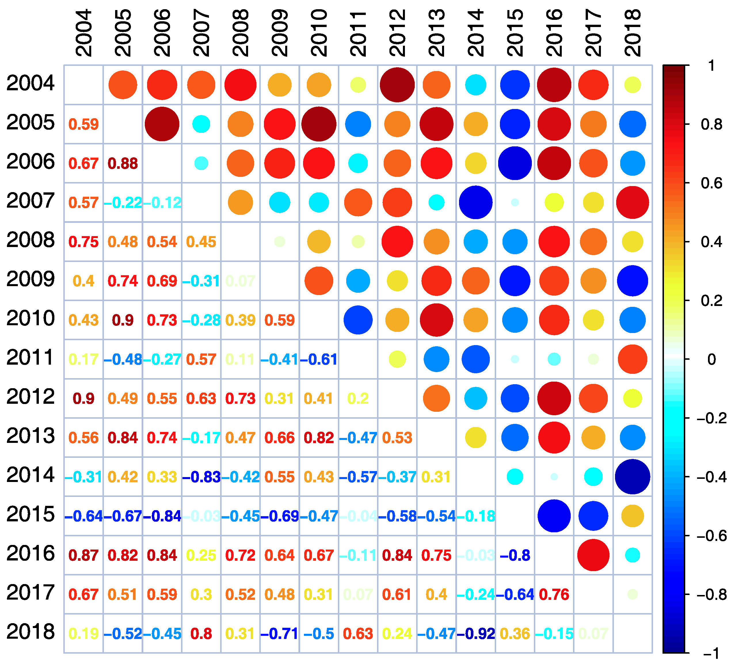
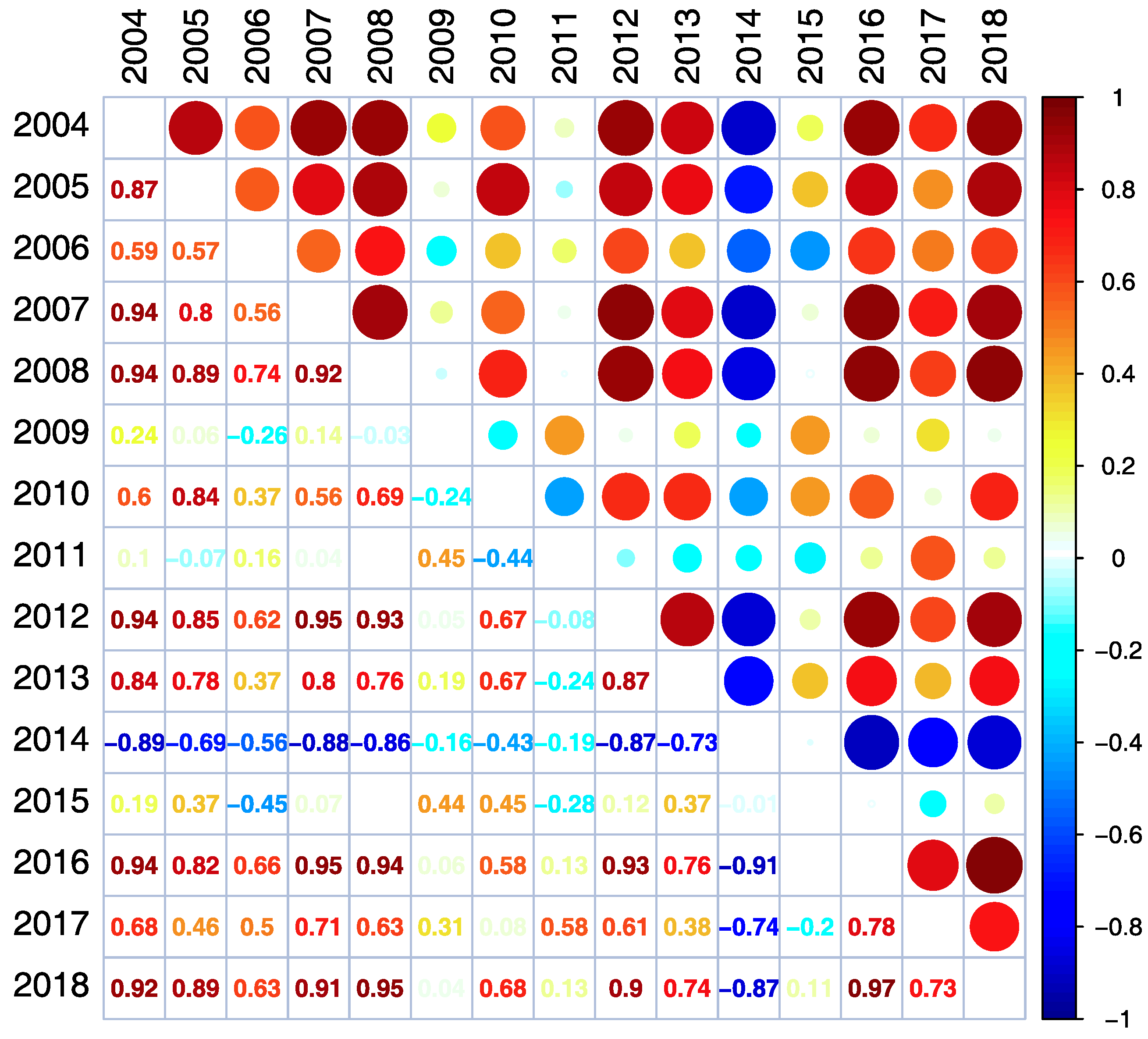
The Pearson correlation matrix for the analyzed data is presented in a graphical correlation matrix, where the size of circles is related to the value of the Pearson correlation between segments; hot colors means positive, while cold colors stand for a negative correlation (Figure 8, Figure 9 and Figure 10). High, positive Pearson correlations can indicate that there is a similar fluctuation of time series of the analyzed segments. We have also analyzed the Pearson correlation matrix for the time series of the groundwater levels corresponding to summer (Figure 9) and winter seasons (Figure 10).

The correlation analysis showed, that there are several groups of HY with similar properties. Within these groups, the correlation is very high, whereas between HYs from different groups, the correlation is much smaller. Correlation coefficients are higher for seasons than for whole years and winter seasons are much more self-similar than summer seasons. One may therefore conclude that the relatively weak annual correlation results from differences in the summer seasons.

An alternative approach to find a similarity between time series is based on clustering. The agglomerative clustering (AHP) is the most popular type of hierarchical clustering. Based on the similarity of the objects, AHP groups the objects into clusters [54] in a “bottom-up” approach. This means that each observation starts in a single-element cluster, and if two clusters are the most similar, they are merged as one moves up the hierarchy. There are many cluster agglomeration methods. In this paper we use the Ward linkage criterion, which minimizes the total variance within clusters. The sum of squares metric is described by the following formula [55]:

$$d(r,s)=\sqrt{\frac{2n_r{n}_s}{(n_r+n_s)}}\left|\right|{\overline{x}}_r-{\overline{x}}_s{\left|\right|}_2,$$

(3)

where r and s are the analyzed clusters, $n_r$ and $n_s$ are the number of elements in clusters r and s respectively, ${\overline{x}}_r=\frac{1}{n_r}{\sum }_{i=1}^{n_r}{x}_{ri}$ and ${\overline{x}}_s=\frac{1}{n_s}{\sum }_{i=1}^{n_s}{x}_{si}$ are the centroids of clusters r and s, respectively and ${\left|\right|·\left|\right|}_2$ is the Euclidean distance. 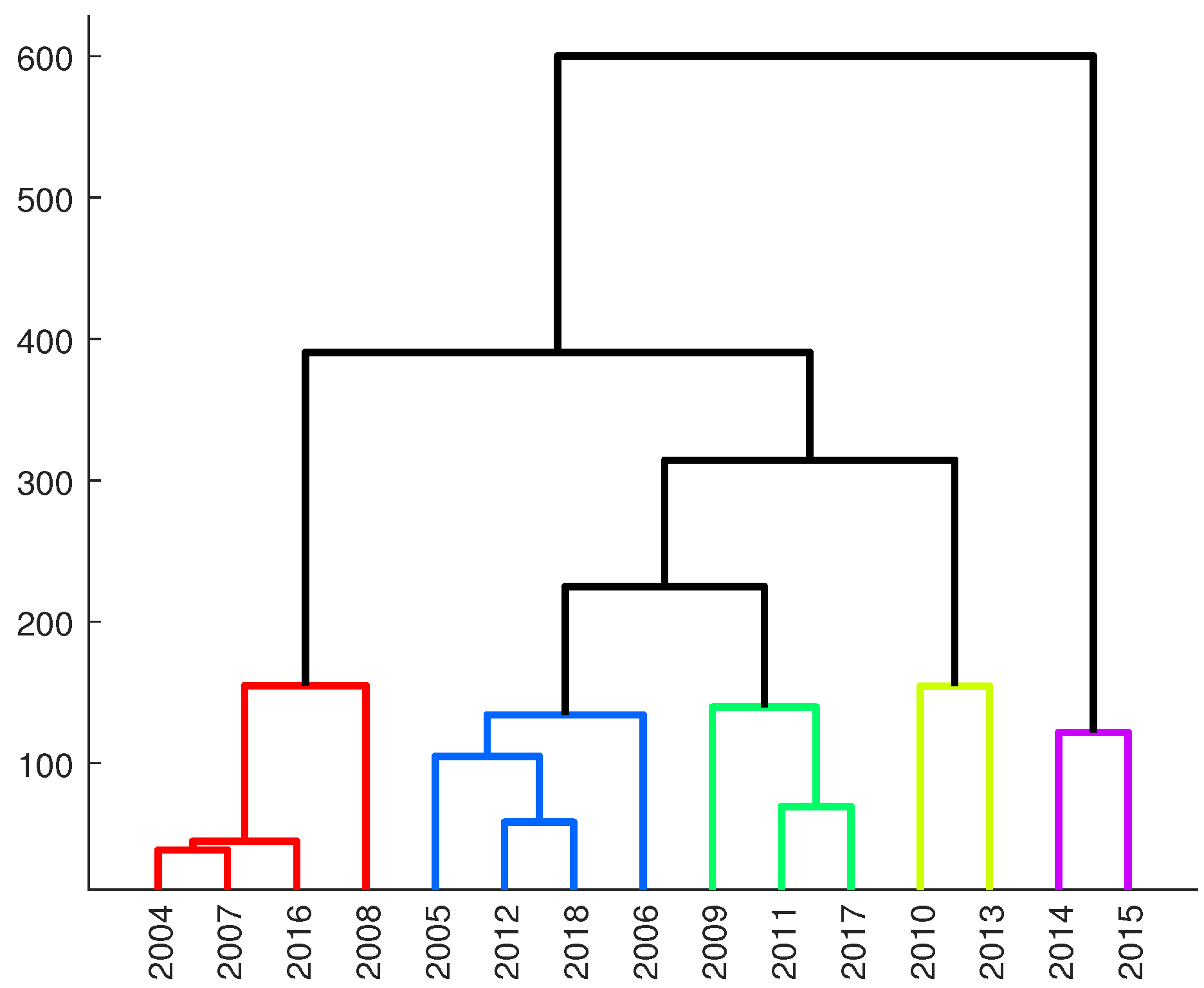In order to estimate the number of clusters, we use the gap statistic [56]. One of the methods to present the results of the AHP is a dendrogram, which is a graphical representation of the clusters produced by the corresponding analyses.

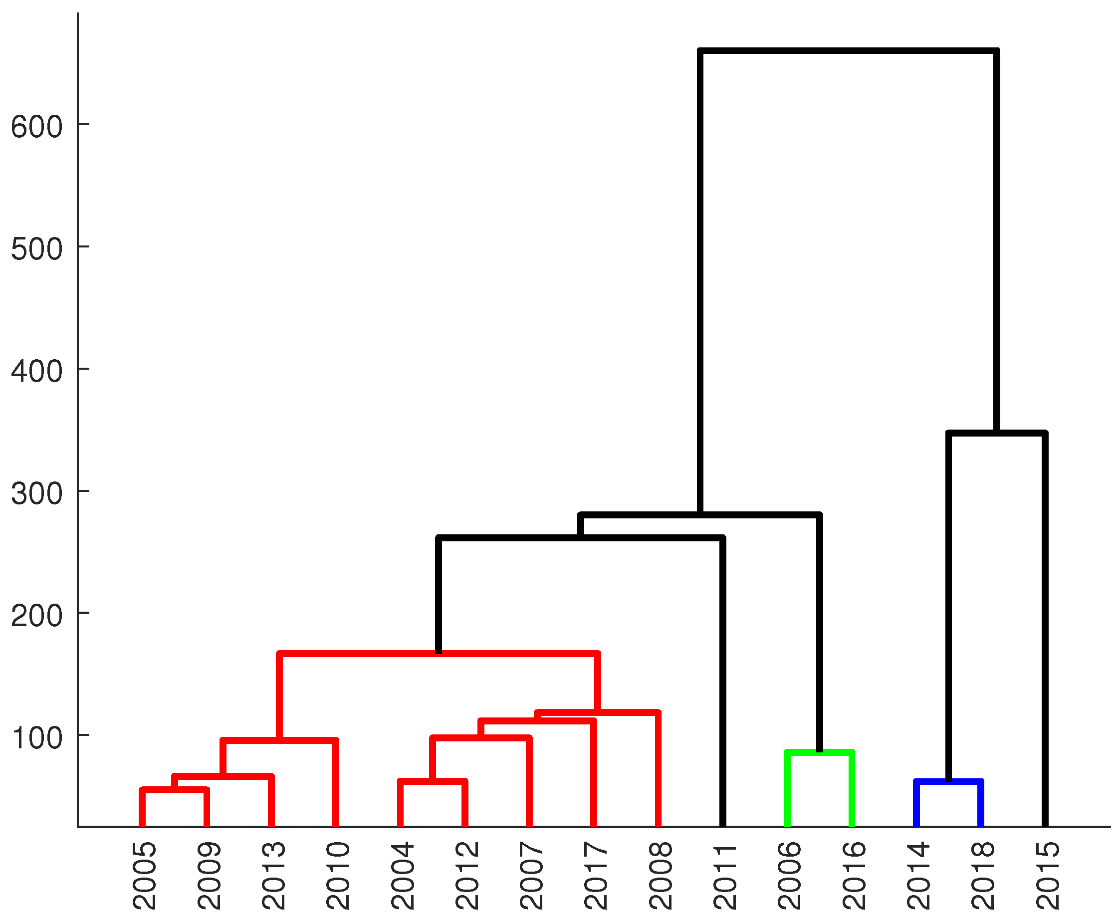
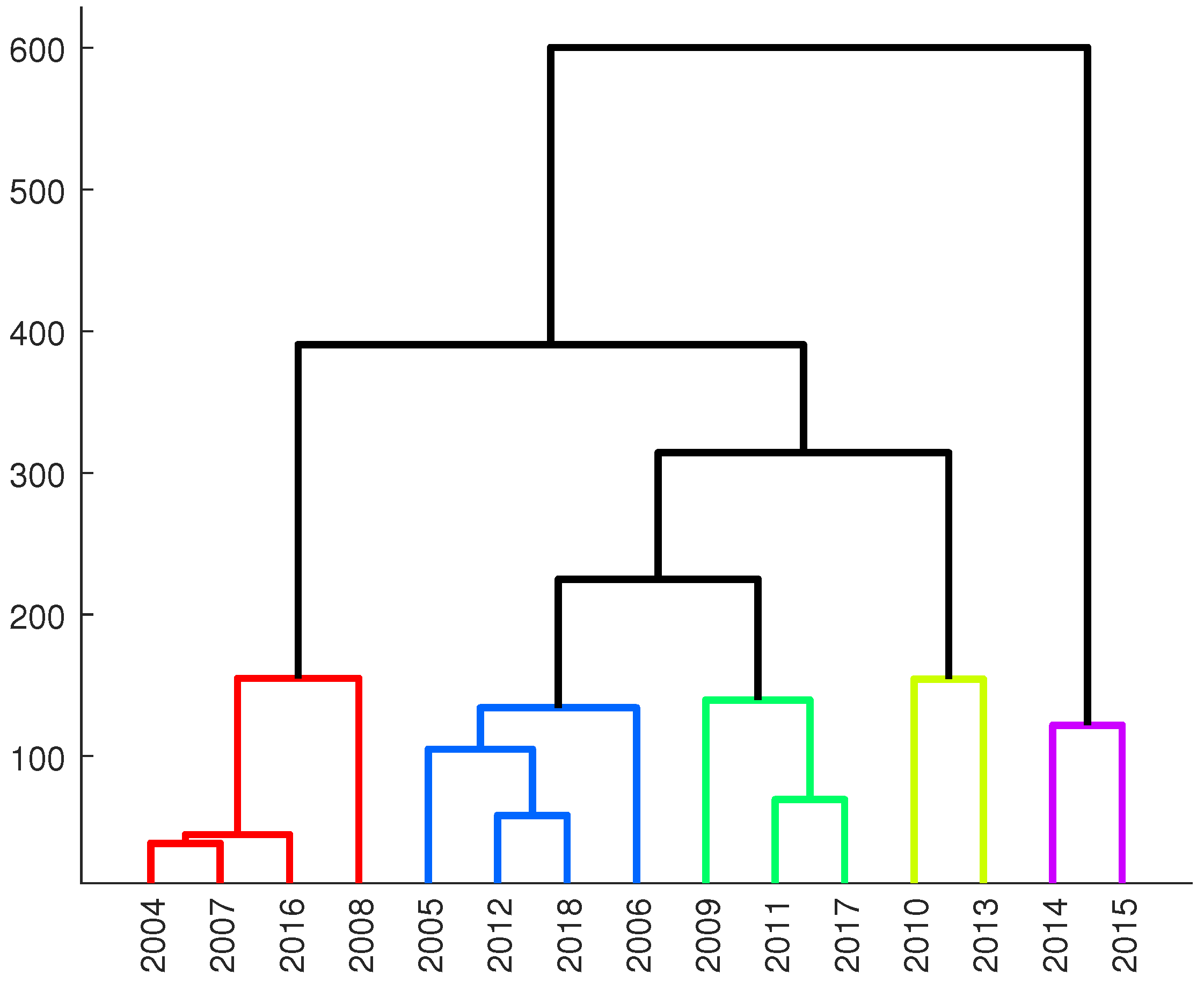
As input data, we provide the same segments as for the Pearson correlation matrix. The dendrogram and year-to-year time series are clustered into 5 groups (Figure 11 and Figure 12, respectively). If there is more than one value in the cluster, they have been marked with color, otherwise they are black. By analogy, AHP clustering has been applied to seasons of the analyzed HYs (Figure 13 and Figure 14 for winter seasons and for summer seasons Figure 15 and Figure 16). One may conclude that both techniques (correlation and clustering) showed that the time series corresponding to the HYs might be very different. The same we observe for winter and summer seasons. Moreover, it might happen that time series of groundwater levels of the HY is different for a half of the year only. This confirms the need to analyze the time series by seasons.

Intuitively, the groundwater level depends on precipitation. Consequently, in the next step, the dependence between the groundwater level and precipitation will be examined to identify a relationship and if it evolves in time. Except for the basic measure of a linear dependence, we also examined the two rank correlation coefficient measures: Kendall tau [57] and Spearman rho [58]. In contrast to the Pearson correlation coefficient, they show the monotonic dependence, not only the linear one. Moreover, due to the specific nature of data, namely the presence of outliers, the quality of dependence measures from several approaches was validated. The Kendall’s tau correlation coefficient of two time series ${\{z_t^i\}}_{t=1}^n$ and ${\{z_t^j\}}_{t=1}^n$ is defined as follows:

$$\tau (z^i,z^j)=\frac{2}{n(n-1)}\sum _{k<l}{d}_{kl}^{z^i}{d}_{kl}^{z^j},$$

(4)

where n is the sample size, $d_{kl}^{z^i}=sign(z_k^i-z_l^i)$ and $d_{kl}^{z^j}=sign(z_k^j-z_l^j)$.

The second considered rank measure is the Spearman rho correlation coefficient. It can be defined based on the Pearson correlation coefficient ($\rho (·,·)$) described in (2) between the rank variables:

$$r(z^i,z^j)=\rho ({rg}_{z^i},{rg}_{z^j}),$$

(5)

where ${rg}_{z^i}$ and ${rg}_{z^j}$ are the ranks obtained from two time series ${z_t^i}_{t=1}^n$ and ${\{z_t^j\}}_{t=1}^n$ respectively.

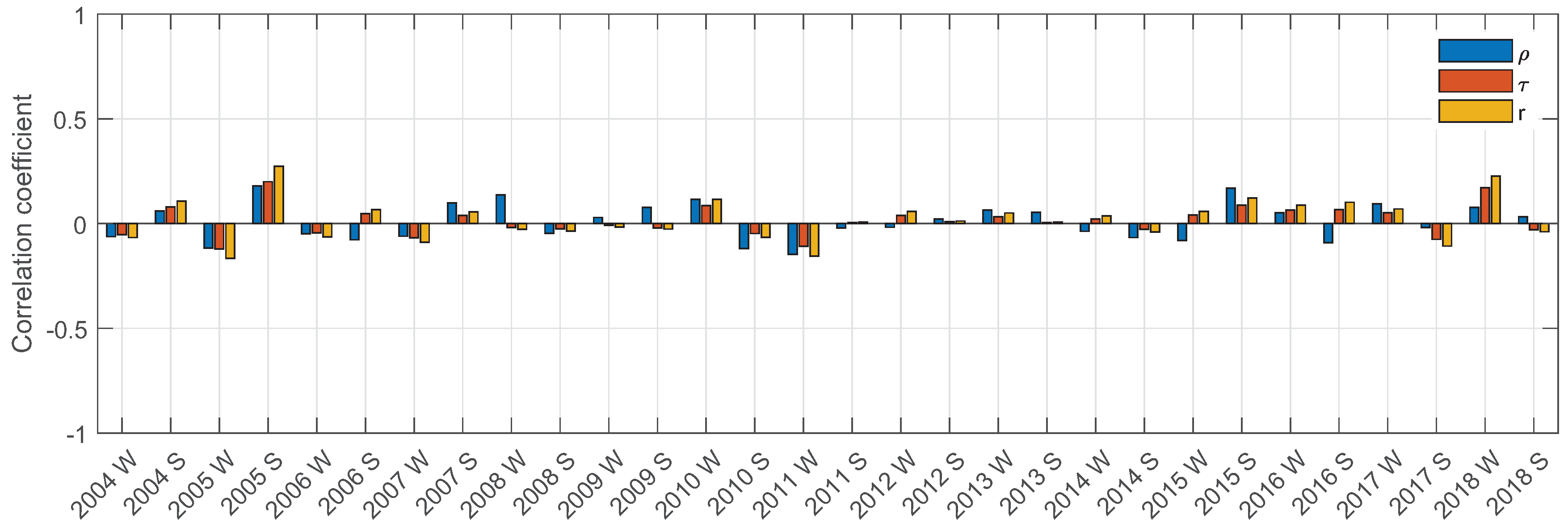
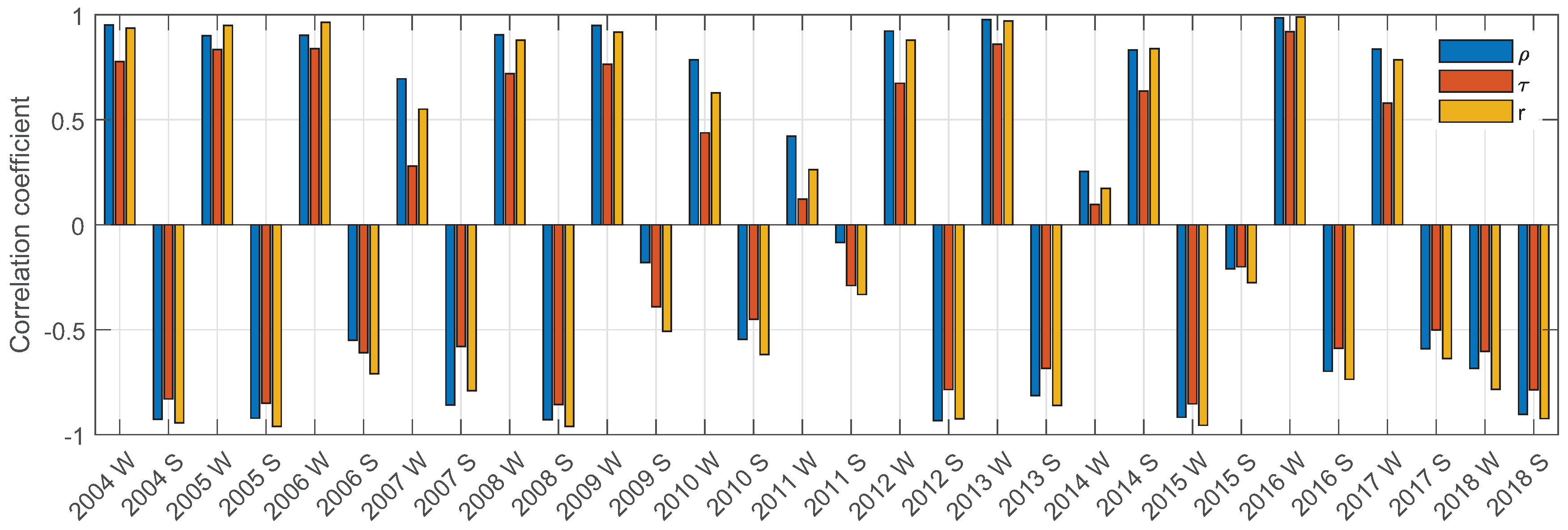
The results obtained for the winter and summer seasons are presented alternately (Figure 17). Based on the results (Figure 17), one might conclude that a relationship between the time series of the groundwater level and precipitation does not exist which seems to contradict the mentioned intuitive expectations.

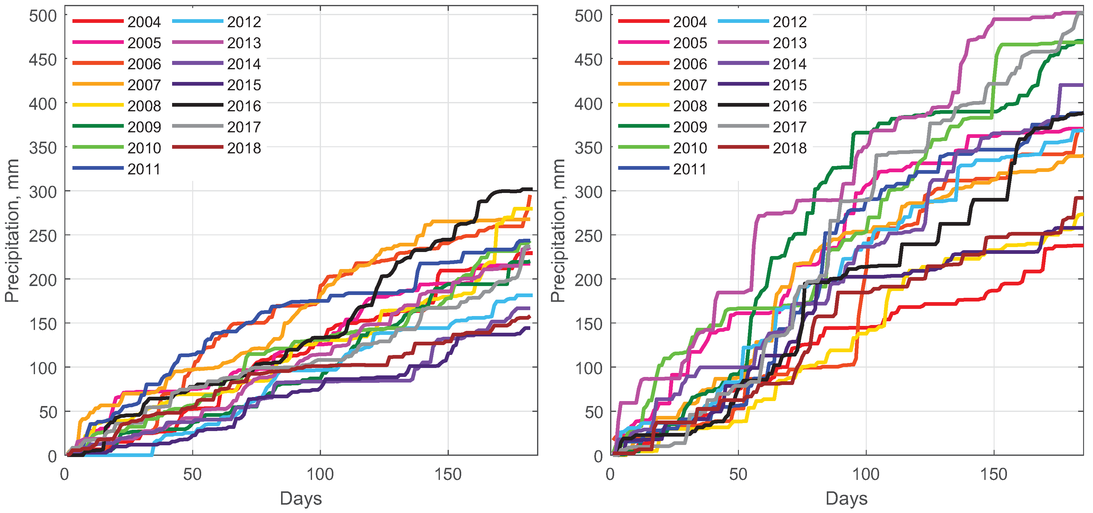
What might be the reason for the small correlation? It seems as if the explanation is hidden in the two data sets (Figure 18). Based on the data, the groundwater level is low at low precipitation periods (up to day 150), and it increases thereafter. This, intuitively, might result in a strong cross-correlation, yet, the statistical analysis does not confirm this observation. Therefore, the relationship between the cumulative sums of the precipitation (CSP) and the groundwater level (Figure 19) was analyzed, where the cumulative sum of the precipitation vector $P(1),\dots .P(N)$ is given by:

$$\mathrm{CSP}(i)=\sum _{k=1}^{i}P(k),i=1,\cdots ,N,$$

(6)

where N is the vector size. The CSP considers also the ”history” of precipitation and indirectly the specificity of the location and the permeability of the ground. Due to different types of pavement, varied geological conditions, specific permeability and actual weather conditions, not all the rain can easily and immediately reach the groundwater table. This happens with a delay and only when there is enough intensive or long-lasting precipitation. 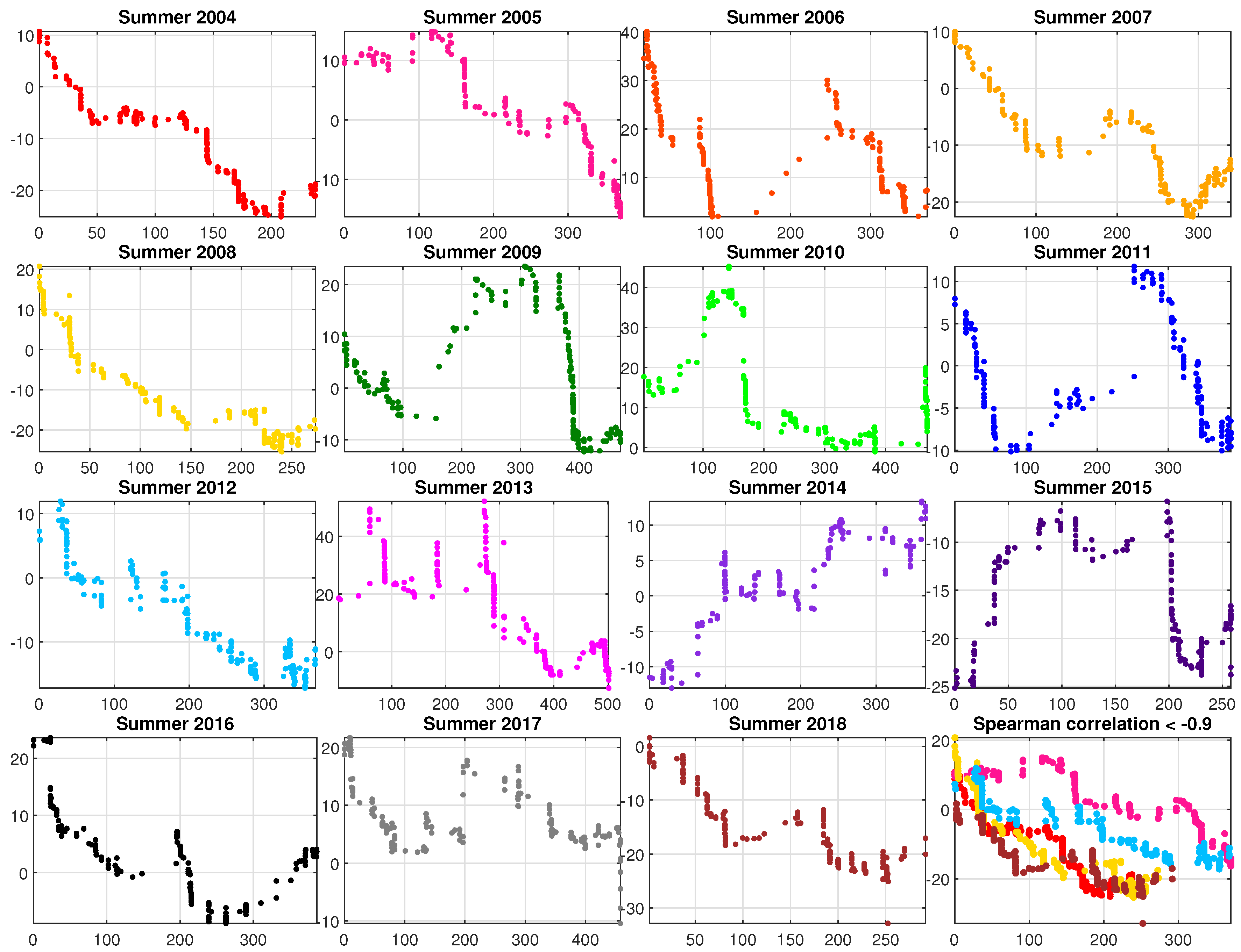Considering a situation, where past precipitation causes an elevated groundwater level in the present, using the cumulative precipitation sum, this dependency can be identified as well (Figure 20). As can be seen, there is a positive dependency in the winter seasons and a negative one for the summer seasons, which will be explained in the Discussion. Although there is generally a strong relation between the groundwater level and the cumulative sum of the precipitation, the dependency is (a) not linear, (b) differs in the annual and seasonal relationships and (c) some years show a high Spearman correlation coefficient (Figure 21 and Figure 22). In addition, though a correlation between the groundwater level and the cumulative precipitation might be expected, there are several years with an unexpected, “abnormal” behaviour.

5. Discussion

Groundwater table fluctuations in Poland have been divided by Pleczyński [59] into four types depending on the geological setting of the observation point and the behavior of the groundwater table during the HY. If the observation point had been located in a undisturbed environment, it would be characterized as the type III (shallow, wide-spread aquifers within river or lake regime characterized by small amplitudes of the groundwater level with a typical increase in the winter season and decrease during the summer season) or as a type IV (shallow aquifers of rivers valleys and terraces with differentiated amplitudes and a few phases of increase and decrease of the groundwater levels during the HY). Which characteristics can be identified in the semi-urban area of Wrocław?

The results of year to year AHP and the Pearson correlation matrix clearly show that some groups of similar HYs and seasons exist. The best option to identify the character of the groundwater level fluctuations and the general shape of the groundwater level diagram during the HY is clustering (Figure 12). Generally, the two largest classes, class 2 (HYs: 2004, 2008, 2012, 2017) and 5 (HYs: 2005, 2006, 2009, 2010, 2013, 2016) can be classified as type III $sensu$ Pleczyński with a rising groundwater level during the winter season, a maximum in the springtime (typically in May) and a falling water table during the summer season. These two classes are mirrored by the green and blue groups in the dendrogram (Figure 11) as well as the Pearson correlation matrix (Figure 8). The HYs 2007, 2011, 2018 combined in class 3 represent the type IV $sensu$ Pleczyński. Groundwater levels in these years have been fluctuating irregularly with several high and lows of the groundwater level. This class is represented in the red group of the dendrogram. Finally, there are the HYs 2014 and 2015 that differ significantly from all the others and are grouped into classes 1 and 4, represented by black lines in the dendrogram.

Seasonal analysis of the HYs shows different results than the yearly ones. The winter seasons’ character is similar to the whole years (Figure 14 and Figure 15): the two largest classes (class 2 and 3) consist of the same years as classes 2 and 3 in the annual clustering. They can be classified as type III $sensu$ Pleczyński and be considered ’typical’ seasons. Class 5 consists of the winter seasons in years 2014 and 2018 and might be Pleczyński’s type IV. Winter seasons 2011 and 2015 are significantly different from all other winters seasons and fall into classes 1 and 4.

Different results have been obtained for the summer seasons analysis (Figure 15 and Figure 16). Two similar and dominant classes 1 and 4 were identified and can be classified as type III $sensu$ Pleczyński. Yet, the individual years do not fall in the same classes as the results of the annual or winter analysis.

What are the implications of these results? Some groundwater fluctuations in the semi-urban area show characteristics that allow the definition of a typical HY. Yet, the results also show a substantial variability in the inter-annual groundwater levels, especially in the summer seasons, and that some HYs deviate significantly from all the other HYs. All these differences might be explained with a deeper investigation of the various factors influencing the groundwater levels (GWL):

$$\mathrm{GWL}=f(R,T,P,U,H,SWL,E,G,A),$$

(7)

where R: precipitation, T: air temperature, P: atmospheric pressure, U: total insolation, H: air and ground humidity, $SWL$: surface water level, E: evapotranspiration, G: geological conditions and ground parameters, and A: anthropogenic influence.

For shallow groundwater in undisturbed conditions, the main factor influencing the groundwater table is precipitation [60]. As has been shown, the groundwater level in the examined HYs 2004–2018 follows the undisturbed cycle in some years, and in others it behaves in a substantially different way. Therefore, the authors have decided to analyse the relationship between the groundwater level and precipitation in that specific case of semi-urban part of Wrocław.

As mentioned above (section Methods and Preliminary Analysis), the influence of the precipitation on the groundwater level appears with a delay and depends on the cumulative rainfall in the examined time period (Figure 20). In the seasonal scatter-plots (Figure 21 and Figure 22) it can be seen that a “typical” hydrological year, as indicated by the AHP analysis, is characterized by a strong correlation between the groundwater level and the precipitation. The winter seasons 2005, 2006, 2009, 2013 and 2016 and summer seasons 2004, 2005, 2008, 2012 and 2018 belong to dominating seasonal groundwater level classes and correlate best with the cumulative sum of the precipitation. It is also obvious that there is some regularity in the positive (usually in winter seasons) and the negative (summer seasons) correlation coefficients (Figure 20) that correspond with the groundwater level increase and groundwater level decrease, in most cases. Exceptions are the winter seasons 2015 and 2018 as well as the summer season of the year 2014. It can also be seen that the groundwater levels in the untypical seasons and years (2011, 2014 and 2015) shows the weakest correlation with the precipitation.

At this stage of the project, we cannot precisely indicate the reasons for these exceptions. There is a need for a deeper analysis of the precipitation-groundwater level relationship, and we suppose these differences might be caused by water level fluctuations of the Odra river and its channels. On the other hand, there might be currently unidentified artificial or natural influences such as pumping or a spatiotemporal influence of precipitation on the groundwater level.

6. Future Work

As has been shown, the analysis of hydrogeological data reveals important, partly unexpected relationships with specific characteristics as in case of the semi-urban part of Wrocław investigated in this paper. This investigation also showed that each data set requires special methods (e.g., segmentation, detrending, denoising or pre-processing). Even when no relevant results are identified during preliminary pre-processing, it might be worth mentioning that some signal processing needs stationary or zero mean processes. In this investigation, the data was sectioned into defined hydrological years and the correlated annual seasons. Yet, the defined starting and end points of the hydrological year might not always be representative for a cycle that can be identified by statistical analysis. Therefore our research question (ii) is still valid, and further studies need to focus on statistical methods that would identify variable starting and end points of cycles that better describe relationships between precipitation and the groundwater levels. This paper also showed that alternative statistical methods are required for further studies. In addition, more variables and multidimensional models need to be used in future studies, as has been shown in the literature study, where autoregressive modelling was used [61]. In the future, it is necessary to understand the groundwater level fluctuations by using prognostic models resulting in a better understanding and improvement of water management in semi-urban areas. In addition, it will be necessary to include more information about the geological and hydrogeological background, such as the strata of the vadose and saturated zones as well as the hydraulic conductivity of the strata. It will also be necessary to include hydrological data of the branches of the Odra river surrounding the island.

7. Conclusions

Daily groundwater level data during a 15 hydrological years period in a semi-urban area of Wrocław, Poland, have been examined with various statistical methods. First research results are presented in this article and show that the used methods for groundwater level fluctuation analysis are viable and allowed to identify patterns typical for a hydrological year. Both, the agglomerative clustering results and the correlation investigations clearly showed that groups of similar groundwater level–precipitation behaviour can be identified for some hydrological years. Typical hydrological year patterns can be influenced by non-identified factors resulting in groundwater level fluctuations that significantly differ from the preceding year. Yet, using data decomposition into winter and summer seasons reveals otherwise unnoticed similarities. In the case of the investigated semi-urban groundwater data, the winter seasons showed clear similarities, while the summer data shows groundwater level fluctuations based on so far unidentified factors.

Thus, referring to the earlier research questions (i) and (iii), we can conclude that: (i) the groundwater level in a semi-urban area does not behave in a similar way every hydrological year and season, but we can indicate some groups of annual and seasonal groundwater level fluctuations and (iii) we defined a typical pattern of groundwater level fluctuations and identified abnormal years, but the question about the reasons for the anomalies is still open.

From the results of this investigation, it can be concluded that a day to day analysis of precipitation and groundwater level fluctuation in a complex system is not possible, though three different correlation methods were applied. These results might be misleading in understanding the groundwater level—precipitation relationship, as there seems to be no direct relationship between these two factors.

Though the general shapes of the groundwater level—precipitation matrix seem to be similar (Figure 18), the correlation is weak. Because of the site-specific conditions, the precipitation needs some time to fill the unsaturated soil column and reach the groundwater level. Therefore, the cumulative sum of the precipitation shows in most cases a better correlation with the groundwater level than the precipitation by itself, in some cases even a linear relationship.

Another result is that positive correlations prevail in the winter season and negative ones in the summer season. We conclude that this negative correlation results from (i) a high insolation and elevated evapotranspiration resulting in a decrease in groundwater recharge and (ii) from effects of the water regulation of the Odra river during the summer seasons or one of each. Challenging, still, are cases where a nonlinear relationship exists.

In conclusion, the results allow identifying relationships between precipitation and groundwater level fluctuations and a classification of hydrological years into a set of classes. The applied statistical and signal processing methods are universal and the assumption about the geological setting of the region is not required. Thus, we can extend the proposed approach to consider for instance the relationship between precipitation and groundwater level for regions of different geological settings and observe if it has an influence on the correlation coefficients.