An Entropy Weight-Based Lower Confidence Bounding Optimization Approach for Engineering Product Design

Abstract

The optimization design of engineering products involving computationally expensive simulation is usually a time-consuming or even prohibitive process. As a promising way to relieve computational burden, adaptive Kriging-based design optimization (AKBDO) methods have been widely adopted due to their excellent ability for global optimization under limited computational resource. In this paper, an entropy weight-based lower confidence bounding approach (EW-LCB) is developed to objectively make a trade-off between the global exploration and the local exploitation in the adaptive optimization process. In EW-LCB, entropy theory is used to measure the degree of the variation of the predicted value and variance of the Kriging model, respectively. Then, an entropy weight function is proposed to allocate the weights of exploration and exploitation objectively and adaptively based on the values of information entropy. Besides, an index factor is defined to avoid the sequential process falling into the local regions, which is associated with the frequencies of the current optimal solution. To demonstrate the effectiveness of the proposed EW- LCB method, several numerical examples with different dimensions and complexities and the lightweight optimization design problem of an underwater vehicle base are utilized. Results show that the proposed approach is competitive compared with state-of-the-art AKBDO methods considering accuracy, efficiency, and robustness.

1. Introduction

Computational simulation models, i.e., finite element analysis (FEA) and computational fluid dynamic (CFD) models, have been widely used in engineering design problems to replace physical experiments for reducing the time cost and shortening the product developing cycle. However, it is still computationally prohibited to solve engineering design optimization problems directly relying on simulation models, even though the storage capacity and computing efficiency of computers are maintaining rapid growth [1,2]. A popular strategy to address this limitation is to adopt surrogate models, also named the meta-model or approximate model, to replace the computational simulation model during the optimization process. There are several varieties of surrogate models, such as Polynomial response surface (PRS) model [3], Radial basis function (RBF) model [4,5], Kriging model [6,7,8], and Support vector regression (SVR) model [9,10]. Among these surrogate models, the Kriging model has been intensively used in engineering design optimization because it can provide not only the predicted value of an un-sampled point but also the predicted confidence interval of the predicted value.

The Kriging model-based design optimization methods can be divided into two types [11]: the off-line type and the on-line type. The off-line type uses all the computational resources to construct the final Kriging model in one time and the model does not update during the optimization process. Therefore, the determination of the sampling plan is crucial because the optimization process may fall into the local optimum region if the number of samples is too small [12]. On the contrary, it would waste computational burden if the number of samples is too large. To solve this dilemma, the on-line type has been developed, in which an initial Kriging model is built in the earlier stage and then new samples are added to update the Kriging model sequentially through certain criteria, e.g., maximum mean square error [13], cross validate error [14], etc., during the design optimization process. The on- line type can significantly reduce the computational burden compared with that of the off-line type because the information of the Kriging model is well utilized [15,16].

The on-line type Kriging model-based design optimization methods are also called adaptive Kriging-based design optimization (AKBDO). The target of AKBDO is to obtain the optimum using less computational cost [17,18]. At the same time, the balance between exploration and exploitation is important because it is critical for searching the global optimum. In detail, exploration means the ability of the algorithm to explore the whole design space for the latent optimal region. On the other hand, exploitation aims to identify the local area around the current optimum. Typically, there are several sorts of adaptive sampling approaches of AKBDO with different ways of making a trade-off between exploration and exploitation [19,20], such as the maximum-uncertainty adaptive sampling approaches [20], the efficient global optimization (EGO) methods [21], the lower confidence bounding (LCB) based methods [22], the aggregate-criteria adaptive sampling methods [19], and the multi-criteria adaptive approaches [23,24]. Among these approaches, the efficient global optimization method proposed by Jones [21] has been intensively adopted to handle realistic product design due to its high efficiency and ease of operation. In this work, the expected improvement (EI) function is introduced to quantify the improvement of an un-known point to the current best solution. The new point can be obtained by maximizing the EI function, and the Kriging model can be updated adaptively by adding the new point to the original sample set. The EI based EGO method has been intensively investigated in recent years [25,26,27]. For example, Xiao [28] proposed a weighted EI to make the balance between exploration and the exploitation more flexible; Zhan [29] proposed the EI matrix method to solve the multi-objective problem. Another famous AKDBO method is the LCB- based method [30]. The LCB function is an effective approach to balance exploration and exploitation by combining the predicted value and variance in a simple way [31]. Subsequently, a parameterized LCB (PLCB) method was proposed by using cool strategy to improve the ability to balance the exploration and exploitation of the original LCB [32]. Cheng et al. [33] considered the coefficient of variation of predicted values and variance to determine the weight factor adaptively during the sequential process. Further, some variants of the LCB methods focus on upper confidence bounding, such as, the Gaussian process upper confidence bounding (GPUCB) algorithm proposed by Srinivas et al., which considers the upper confidence bound of noisy functions [34]. The parallel type of the GPUCB was developed by Desautel et al. [35]. It mentions that LCB methods have been widely applied to solve real engineering problems [36,37]. However, the weight factor for balancing the exploration and the exploitation of the LCB based method remains an interesting problem. This is because most of the existing factor approaches are subjective or problem dependent, which is not robust in application for all cases.

In this paper, an entropy weight-based lower confidence bounding approach (EW-LCB) is proposed to ascertain the weight of the LCB function adaptively and objectively. In the proposed EW-LCB method, entropy theory is used to quantify the degree of variation of the predicted value and variance of the Kriging model. Then, a new weighted formula is introduced to allocate the weights of exploration and exploitation adaptively. To validate the performance of the proposed EW- LCB method, several numerical functions with different dimensions and complexities and an engineering problem are tested. The computational efficiency, accuracy of the optimum, and the robustness are considered when comparing EW-LCB with the existing famous AKBDO methods. Results showed that the performances of the proposed EW-LCB approach were competitive on the test cases.

The remainder of this paper is organized as follows, in Section 2, the basis of the Kriging model and several existing famous AKBDO methods are introduced. The details of the proposed approach with the assistance of an illustrative example are described in Section 3. In Section 4, the effectiveness of the proposed approach is tested on several numerical benchmark problems and an engineering design optimization problem. Finally, some conclusions and possible future works are proüposed in Section 5.

2. Background

2.1. Kriging Model

The Kriging model was originally proposed by Krige [38] to predict the location of a mine hole in a geostatistical community. Then, it was extended by Sacks et al. [6] for modeling an experiment of a computer. The Kriging model is also called the Gaussian process model, which is a kind of interpolative model. The Kriging model can be expressed as

$$\widehat{y}(\mathit{x})=\beta +Z(\mathit{x})$$

(1)

where $\mathit{x}$ represents the vector of the design variables, which is a d-dimensional vector $\mathit{x}=\left\{x_1,x_2,\dots ,x_d\right\}$, $\beta$ is an unknown parameter which denotes the global tendency, $Z(•)$ is a static Gaussian process with zero mean and non-zero variance ${\sigma }^2$, which represents the local deviation.

In the static Gaussian process, spatial correlation is used to organize the relationship between any two samples. Generally, the squared exponential function is utilized, which can be expressed as

$$R({\mathit{x}}_i,{\mathit{x}}_j;\mathit{\theta })=\exp (-{\displaystyle \sum _{k=1}^d{\theta }_k{(x_i^k-x_j^k)}^{p_j}})$$

(2)

where $\mathit{\theta }$ and $\mathit{P}$ are the hyper-parameters used to control the smooth and the correlation between two sample points. Generally, the hyper-parameter vector $\mathit{P}$ is set to be $p_i=2;i=1,2,\dots ,d$ [39].

The core point of the modeling process of the Kriging model is to determine the unknown parameters. Because the responses obey the multivariable Gaussian distribution, the unknown parameter can be obtained by maximum likelihood estimation (MLE) [14]. The likelihood function can be organized as

$$L\left(y({\mathit{x}}_1),y({\mathit{x}}_2),\dots ,({\mathit{x}}_N)|\sigma ,\beta ,\mathit{\theta }\right)=\frac{1}{{(2\pi {\sigma }^2)}^{\raisebox{1ex}{$N$}\!\left/ \!\raisebox{-1ex}{$2$}\right.}}\exp \left[-\frac{{\displaystyle \sum _{i=1}^N{(\mathit{y}({\mathit{x}}_i)-\beta )}^2}}{2{\sigma }^2}\right]$$

(3)

where $N$ is the number of samples.

Then, Equation (3) can be simplified by taking the natural logarithm,

$$\ln \left(L\right)=-\frac{N}{2}\ln (2\pi )-\frac{N}{2}\ln \left({\mathsf{\sigma }}^2\right)-\frac{1}{2}\ln \left(\left|\mathit{R}\right|\right)-\frac{{(\mathit{y}-\mathbf{1}\beta )}^T{\mathit{R}}^{-1}(\mathit{y}-\mathbf{1}\beta )}{2{\mathsf{\sigma }}^2}$$

(4)

where $\mathit{y}$ is an N-dimensional vector that consists of the real responses, $1$ is an N-dimensional vector that consists of 1,

The values of $\beta$ and ${\mathsf{\sigma }}^2$ can be obtained by setting the derivatives of Equation (4) concerning $\beta$ and ${\mathsf{\sigma }}^2$ to be 0,

$$\widehat{\beta }=\frac{{\mathit{f}}^{\mathit{T}}{\mathit{R}}^{-1}\mathit{y}}{{\mathit{f}}^{\mathit{T}}{\mathit{R}}^{-1}\mathit{f}}$$

(5)

$${\widehat{\sigma }}^2=\frac{{\left(\mathit{y}-\mathbf{1}\widehat{\beta }\right)}^T{\mathit{R}}^{-\mathbf{1}}\left(\mathit{y}-1\widehat{\beta }\right)}{N}$$

(6)

Then, substituting Equations (5) and (6) into Equation (4), and remove the constant terms, Equation (4) yields the concentrated ln-likelihood function

$$\ln (L)=-\frac{N}{2}\ln \left({\widehat{\sigma }}^2\right)-\frac{1}{2}\ln \left(\left|\mathit{R}\right|\right)$$

(7)

It is difficult to obtain an analytical solution of $\mathsf{\theta }$ because of high non-linearity and non-differentiality. Therefore, a numerical solution is obtained instead. The optimization algorithm, such as the genetic algorithm (GA) [40] and particle swarm optimization algorithm (PSO) [41], can be used to find the optimized values of $\mathsf{\theta }$.

The Kriging model is widely adopted in surrogate model-based engineering optimization because it can provide both the predicted value and variance [42]. The predicted value of an un- sampled point can be determined by minimizing the mean square error. Thus, the predicted value and variance can be expressed as

$$\widehat{y}(\mathit{x})=\widehat{\beta }+\mathit{r}{(\mathit{x})}^T{\mathit{R}}^{-\mathbf{1}}\left(\mathit{y}-1\widehat{\beta }\right)$$

(8)

$${\widehat{s}}^2(\mathit{x})={\widehat{\sigma }}^2\left[1-\mathit{r}{(\mathit{x})}^T{\mathit{R}}^{-\mathbf{1}}\mathit{r}(\mathit{x})+\frac{{(\mathbf{1}-{\mathbf{1}}^T{\mathit{R}}^{-\mathbf{1}}\mathit{r}(\mathit{x}))}^2}{{\mathbf{1}}^T{\mathit{R}}^{-\mathbf{1}}\mathbf{1}}\right]$$

(9)

where $\mathit{r}(\mathit{x})$ is an N-dimensional vector representing the spatial correlation between the un-sample point and the sample points, which can be defined by

$$\mathit{r}(\mathit{x})=\left\{R(\mathit{x},{\mathit{x}}_1),R(\mathit{x},{\mathit{x}}_2),\dots ,R(\mathit{x},{\mathit{x}}_N)\right\}$$

(10)

2.2. Review of the Typical Adaptive Surrogate-Based Design Optimization Methods

The goal of the AKBDO methods is to obtain the optimum with a limited computational budget. In this section, four popular AKBDO methods are briefly introduced.

2.2.1. The Lower Confidence Bounding Method

With a concise expression, the LCB method is a popular AKBDO method, which can be expressed as

$$lcb(\mathit{x})=\widehat{y}(\mathit{x})-b\widehat{s}(\mathit{x})$$

(11)

where $\widehat{y}(\mathit{x})$ and $\widehat{s}(\mathit{x})$ are the predicted value and standard deviation, respectively. $b$ is a factor utilized to control the weight between the $\widehat{y}(\mathit{x})$ and $\widehat{s}(\mathit{x})$ for the sake of balancing the exploration and the exploitation.

The goal of the LCB function is to identify the new sample points through the combination of predicted value and variance by Equation (11). The point with small predicted value or large uncertainty is chosen. Generally, a larger $b$ means more emphasis on global exploration. On the contrary, with a small $b$ value, the algorithm turns more attention to local exploitation. Cox and John reported that b = 2 and b = 2.5 can give a more efficient search [43].

2.2.2. The Parameterized Lower Confidence Bounding Method

The weight factor in the LCB method is constant, indicating that the contributions of the predicted value and standard deviation will be fixed during the optimization process. Thus, the parameterized lower confidence bounding (PLCB) method is proposed [32], which can be defined by

$$plcb(\mathit{x})=a_i\widehat{y}(\mathit{x})-b_i\widehat{s}(\mathit{x})$$

(12)

where a new parameter $a_i$ is developed to regulate the influence of the predicted value during the iteration process of design optimization. Meanwhile, the values of $a_i$ and $b_i$ vary during the iteration process, where $i$ is the iteration order of the sequential process. In detail, the values of the parameters $a_i$ and $b_i$ can be expressed as

$$a_i=1,b_i=\left(1+\cos \left(\frac{i\pi }{m}\right)\right)/\sin \left(\frac{i\pi }{m}\right)$$

(13)

where $m$ is a parameter defined by the user, it is set to be $m=3$ in Ref. [32].

According to Equation (12), the algorithm tends to focus on exploration when $b_i/a_i$ has a larger value, while it tends to focus on exploitation when $b_i/a_i$ has a respective small value. Specifically, the value of $b_i/a_i$ in PLCB function has a larger value at the former iterations and has a relatively small value as the algorithm goes on. Consequently, the PLCB algorithm shows a better ability to balance the exploitation and the exploration when compared with the LCB method.

2.2.3. The Expected Improvement Method

The expected improvement method is a famous AKBDO method proposed by Jones [21]. The expected improvement function can be defined to measure the latent improvement of an unknown point to the current optimum, which can be expressed as

$$I(x)=\max (y_{\min }-Y(x),0)$$

(14)

The expected improvement can be formalized as

$$E(I(\mathit{x}))=E(\max (y_{\min }-Y(\mathit{x}),0))$$

(15)

which can be expanded into

$$E[I(\mathit{x})]=(f_{\min }-\widehat{y}(\mathit{x}))\Phi \left(\frac{f_{\min }-\widehat{y}(\mathit{x})}{s(\mathit{x})}\right)+\widehat{s}(\mathit{x})\varphi \left(\frac{f_{\min }-\widehat{y}(\mathit{x})}{\widehat{s}(\mathit{x})}\right)$$

(16)

where $\Phi$ and $\varphi$ are the cumulative density function and probability density function of the standard normal distribution, respectively.

According to Equation (16), the first term mainly focuses on the exploitation and the second term primarily concerns the exploration. The point with the maximum value of the EI function is regarded as the new sample to update the Kriging model during the iteration process.

2.2.4. The Weighted Expected Improvement Method

Although the EI method can balance the exploration and the exploitation, its efficiency is problem-dependent because the EI method provides a fixed compromise between the exploration and the exploitation. To address this issue, a weighted expected improvement method (WEI) [28] is developed, in which a tunable weight is adopted to adjust the contributions of exploration and exploitation. The WEI can be given by

$$E[I(\mathit{x})]=w(f_{\min }-\widehat{y}(\mathit{x}))\Phi \left(\frac{f_{\min }-\widehat{y}(\mathit{x})}{s(\mathit{x})}\right)+(1-w)\widehat{s}(\mathit{x})\varphi \left(\frac{f_{\min }-\widehat{y}(\mathit{x})}{\widehat{s}(\mathit{x})}\right)$$

(17)

where $w$ is the weight coefficient. The larger value of $w$ indicates that the WEI will focus more on exploitation. Otherwise, the WEI method emphasizes exploration.

3. Proposed Approach

The goal of the proposed lower confidence bounding approach based on the entropy weight algorithm (EW-LCB) is to obtain an optimal solution with less computational burden through a sequential process. In EW-LCB, a new-weight factor is developed, which can allocate factors to balance global exploration and local exploitation by quantifying the degree of variation of the predicted value and variance from the Kriging model, respectively. In detail, the entropy theory is adopted to evaluate the relative discrepancy between the predicted value and uncertainty of the Kriging model. The framework of the EW-LCB is shown in Figure 1, which is composed of six steps.

To demonstrate the proposed EW-LCB approach more intuitively and detailed, a one- dimensional toy example is utilized. The test function is adopted from [33], which can be expressed as

$$y=0.5\sin \left(4\pi \sin \left(x+0.5\right)\right)+\frac{1}{3}{\left(x+0.5\right)}^2;x\in \left[0,1\right]$$

(18)

The objective is to obtain the minimum value of Equation (18). Meanwhile, this function has a local optimal value $y=-0.0445$ at $x=0$ and a global optimal value $y=-0.1341$ at $x=0.5312$.

The details of the steps are elaborated as follows:

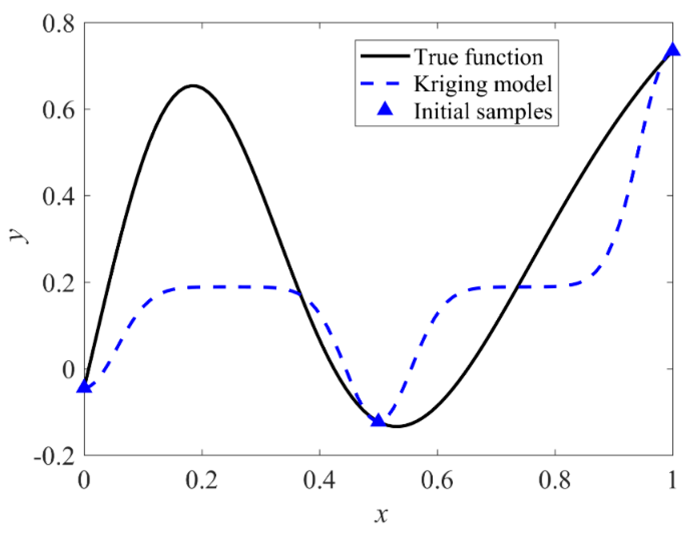
3.1. Step 1: Generate the Initial Sample Set

The generation of the initial sample set includes the determination of the number and location of the initial sample points, which is a crucial component of the AKBDO. If too few points are generated, the AKBDO can have a risk of falling into the local optimal because of the poor accuracy of the initial Kriging model. On the other side, it may be a waste of computational burden if too many initial samples are utilized, especially when dealing with costly engineering problems. For the tested cases, a state-of-the-art initial sample size rule $N=10\times d$ is used [21,44]. The sensitive analysis of the initial sample size is discussed in the next section. Besides, how to allocate the locations of the initial samples is another tricky issue. More uniformed distributed sample points are preferred because the initial Kriging model can obtain more information about the landscape of the real function. Therefore, the Latin Hypercube sampling (LHS) method [45] is used, which can guarantee that the samples distribute along each dimension uniformly.

Due to the simple landscape of the illustration example, the initial sample points are set to be $x=[0,0.5,1]$, which is less than the recommended initial sample size. Herein, the responses of the initial sample points are $y=[-0.0445,-0.1229,0.7343]$, which are obtained by calculating the numerical function in Equation (18).

3.2. Steps 2 and 3: Constructing the Kriging Model and Obtaining the Current Optimal Solution

In Step 2, the Kriging model is established based on the initial sample set based on the DACE toolbox [46]. In detail, the regression function, the correlation function, and the initial value of $\mathit{\theta }$ are set to be ‘Regpoly0’, ‘Corrgauss’, and ${\left(10d\right)}^{-1/d}$, respectively. Besides, all the codes are executed based on the computational platform with a 4.2 GHz Intel(R) Eight-Core (TM) i7-7700k Processor and 64 GB RAM. The initial Kriging model of the illustrated example is plotted in Figure 2 in which, the black line and blue dash line denote the real function and the initial Kriging model, respectively. Meanwhile, the initial sample points are marked with blue triangles.

In Step 3, the current optimal value was obtained through a genetic algorithm [47], where the parameter setting is listed in

Table 1. The parameter setting of the genetic algorithm.

Parameter	Values
Population Size	100
Maximum generation	100
Crossover probability	0.95
Mutation probability	0.01

.

The minimum value of the current responses is $-0.1229$, which is larger than the actual global optimal solution. Then, the current minimum value will be judged by the stopping criterion to decide whether the active-learning process goes on or not in the next step.

3.3. Step 4: Check the Terminal Condition

Generally, there are two common ways to stop the sequential process. That is (1) the difference between the current optimal solution and the actual one achieves at an acceptable level and (2) all the computational resources are used up. In this work, these stopping criteria are adopted for different scenarios. For the numerical functions, because the actual optimal solution is known, the stopping criterion can be associated with this value to test the effectiveness of the proposed approach. Therefore, the stop condition is defined as

$${\epsilon }_r=\left|\frac{\min \left(y_k\left({\mathit{x}}_i\right)\right)-y^r}{y^r}\right|<{\epsilon }_g\hspace{1em}i=1,2,\cdots ,N$$

(19)

where $\min \left(y_k\left({\mathit{x}}_i\right)\right)$ is the minimum value of the current sample set, $y^r$ is the actual optimal solution, ${\epsilon }_g$ is a user-defined tolerance. Generally, the adaptive algorithm will confront the stricter test in the case of smaller tolerance. In this work, the value of ${\epsilon }_g$ is defined as 0.002 referring to [32].

However, for the engineering cases, the above stopping criterion for the numerical problem is impractical because the engineering problem is always a black-box problem. Thus the value of the actual optimal solution is unknown. Therefore, the sequential updating process terminates when the maximum iteration is reached, which can be expressed as

$$k\ge K$$

(20)

where $k$ and $K$ denote the current iteration and the maximum iteration, respectively.

If the stopping criterion is satisfied, the sequential process will be terminated and the algorithm goes to Step 6. Otherwise, the proposed algorithm goes to Step 5 for a new iteration. In this illustrated example, the relative error between the current optimal solution and the actual one is 0.00084. Therefore, the sequential process goes to Step 5.

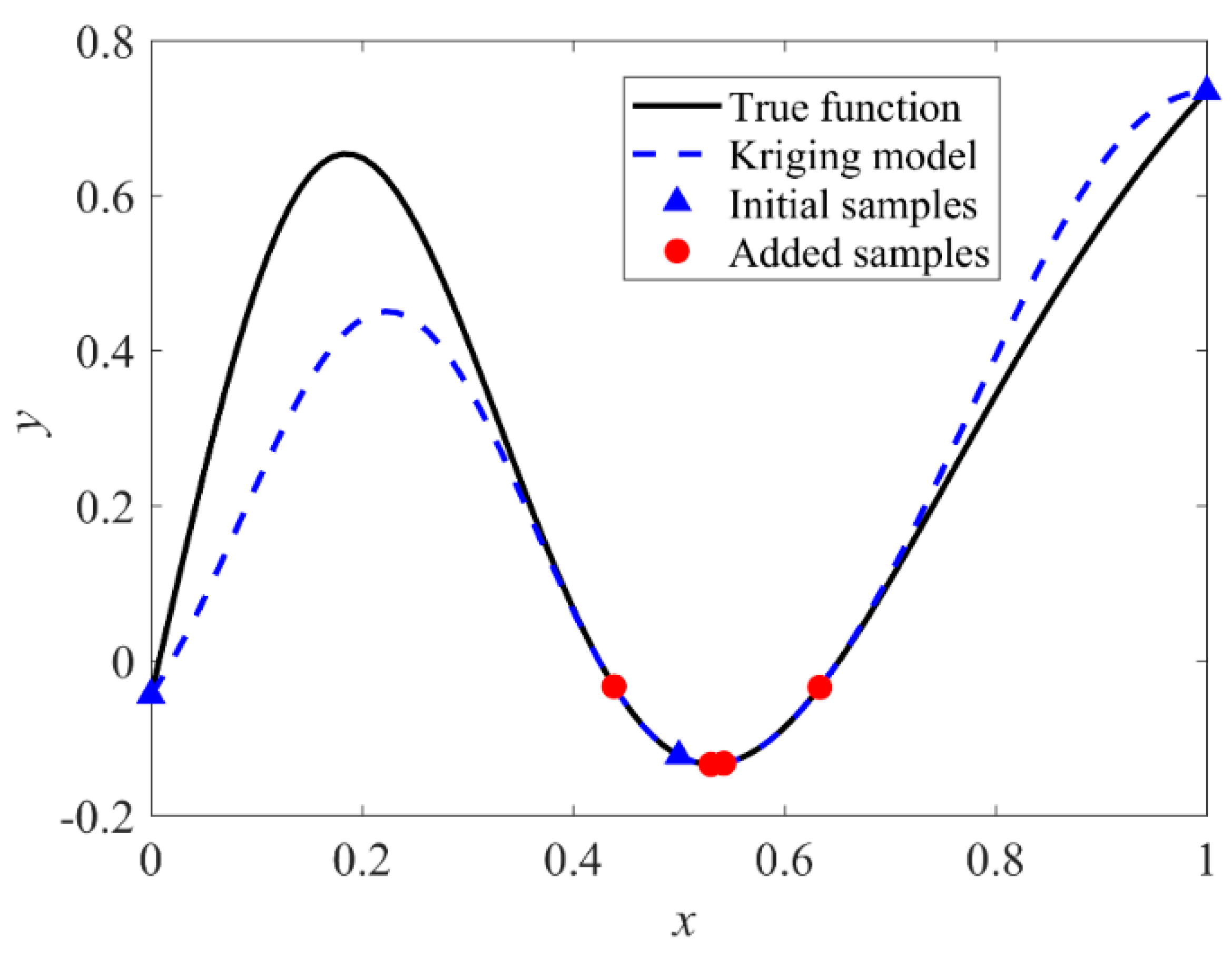
3.4. Steps 5: Update the Sample Set through the Proposed EW-LCB

To accelerate the adaptive optimization process, the lower confidence bounding function based on entropy theory is developed. Entropy theory was proposed by Shannon to quantify the degree of chaos in molecular motion [48,49]. In this work, it is developed to quantify the degree of variation of the predicted value and variance in the sequential optimization process. Herein, the proposed entropy weight method is an objective weighting method, which adaptively assigns weight to the LCB function according to the degree of variation of the predicted value and variances. Specifically, the entropy weight method consists of three major steps: normalize the values of the predicted value and variances, calculate the entropy value of the predicted value and variances, and determine the relative weight of them.

The EW-LCB function is defined as

$$EWMLCB(x)=w_1\widehat{y}(x)-w_2\widehat{s}(x)\exp ({(-1)}^{r}r)$$

(21)

where $\widehat{y}(x)$,$\widehat{s}(x)$ are the predicted value and estimated standard deviation of the tested point, respectively. $w_1,w_2$ are the weights to reflect the contribution of the $\widehat{y}(x)$,$\widehat{s}(x)$, respectively. $r$ represents the iterations of the current optimization solution, which can be used to avoid the proposed approach falling in the local optimal region.

To obtain the weights $w_1,w_2$, suppose that there are $N$ samples with $m$ indexes. The information of the samples can be normalized by

$$Y_{ij}=\frac{X_{ij}-\min \left\{X_{1j},X_{2j},\dots ,X_{Nj}\right\}}{\max \left\{X_{1j},X_{2j},\dots ,X_{Nj}\right\}-\min \left\{X_{1j},X_{2j},\dots ,X_{Nj}\right\}}$$

(22)

where $X_{ij}$ represents the $j^{th}$ index of the $i^{th}$ sample. Equation (22) is used to normalize the lower and upper bound. In this work, the value of $m$ equals 2. Besides, the number of tested points is set to be 1000 to improve the robustness of the entropy weight method.

Then, the entropy value of each index can be determined by

$$E({\mathit{p}}_j)=-\frac{1}{\ln (N)}{\displaystyle \sum _{i=1}^N{\mathit{p}}_{ij}\ln ({\mathit{p}}_{ij})}\hspace{1em}j=1,2,\cdots ,m$$

(23)

where

$${\mathit{p}}_{ij}=Y_{ij}/{\displaystyle \sum _{i=1}^N{Y}_{ij}}$$

(24)

If the value of ${\mathit{p}}_{ij}=0$, it indicates that the entropy of this tested point equals zero. In that case, a definition is given to compensate for the insufficiency of the initial assumption in Equation (23), which is defined as

$$\underset{{\mathit{p}}_{ij}\to 0}{\lim }{\mathit{p}}_{ij}\ln ({\mathit{p}}_{ij})=0$$

(25)

According to Equation (23), the degree of variation of each indicator can be ascertained. The indicator with a larger value of information entropy has a smaller degree of variation. Subsequently, the corresponding entropy weight should be small. As such, the entropy weight can be obtained by

$$w_j=\frac{1-E(P_j)}{{\displaystyle \sum _{j=1}^m(1-E(P_j))}}$$

(26)

According to Equation (26), the weight of each index can be determined adaptively. Besides, $w_j\in [0,1]$ and ${\displaystyle \sum w_j}=1$.

Here we give a brief explanation of the proposed EW-LCB criterion. The term $w_1\widehat{y}(x)$ is used for local exploitation, which concerns the optimal value. On the other side, the term $w_2\widehat{s}(x)\exp ({(-1)}^{r}r)$ focuses on global exploration, which pays more attention to the uncertainty of the Kriging model for the potential global optimal region. If $w_1\ll w_2\exp ({(-1)}^{r}r)$, it means the algorithm focuses more on global exploration. While $w_1\gg w_2\exp ({(-1)}^{r}r)$ means the algorithm focuses more on local exploitation. The factor $\exp ({(-1)}^{r}r)$ serves as the catalyst to help the optimization process out of a local optimization solution. However, this factor may decrease the convergence speed of the proposed algorithm because the weight of the exploration will dominate $EWLCB(\mathit{x})$ when the current optimization solution is repeated too many times. Finally, the point with the minimum value of $EWLCB(\mathit{x})$ is selected as the new update point.

In this illustrated example, the weight parameters are $w_1=0.4961,w_2\exp ({(-1)}^{r}r)=0.5039$ in the first iteration. It is shown that the algorithm focuses more on global exploration than local exploitation. Therefore, another sample point $\mathit{x}=0.4432$ is added, and the corresponding Kriging model is refreshed, which is shown in Figure 3.

3.5. Step 6: Output the Optimal Solution

Once the terminal conditions are achieved, the optimal solution will be the output. As shown in Figure 4, the optimal solution $x=0.5312$ is obtained, which equals the global minimum.

As shown in Figure 4, the trend of the actual function is recognized by the proposed approach and the optimal value can be obtained although the global accuracy of the Kriging model is not at a high level.

For comparison, four AKBDO methods, Expected improvement infill criterion (EI) [21], weighted expected improvement infill criterion (WEI) [28], Lower confidence bounding infill criterion (LCB) [22], and Parameterized lower confidence bounding (PLCB)[32], were tested on this case. To avoid the randomness of the LHS and GA, all the methods were repeated 100 times. The statistical results including the mean value and standard deviations of the function calls are summarized in

Table 2. Comparison results of different approaches of the illustrated example.

Methods	EI	WEI	LCB	PLCB	EW-LCB
Mean Value	7.64	7.86	7.98	7.66	6.48
Standard deviations	1.352	1.498	1.301	1.780	0.505

.

As listed in Table 1, the average number of function calls of the proposed approach is less than those of the four AKBDO methods, indicating that the proposed EW-LCB approach performs better than the four AKBDO methods concerning efficiency. Besides, the standard deviation of the proposed EW-LCB approach is the smallest among all the methods, which means that the proposed approach has the best robustness among all the compared methods in this demonstration case.

4. Tested Cases

4.1. Numerical Examples

In this subsection, ten widely used benchmark problems from Ref. [33,50,51,52] are used to illustrate the effectiveness of the proposed EW-LCB method. Meanwhile, four famous AKBDO approaches, EI, WEI, LCB, and PLCB, are tested to compare with the EW-LCB method. As the optimal solutions for all benchmark problems can be obtained, the terminal condition is defined such that the relative error between the optimal solution obtained from the Kriging model and the true one is within 0.002. Therefore, the number of iterations is regarded as the merit of effectiveness. Considering the randomness of the results, many AKBDO approaches repeat their algorithms dozens of times and provide statistical results [53,54]. Furthermore, some approaches use the deterministic sampling and optimization algorithms such as Hammersley and deterministic PSO [55,56,57] to avoid the randomness. In this work, each method ran 100 times with different initial samples and their statistical results are recorded in

Table 3. The comparison of statistical optimization results.

Functions	Items	EI	WEI	LCB	PLCB	EW-LCB
PK	FEmean	29.82/3	30.13/4	29.68/2	31.99/5	26.97/1
	FEstd	2.435/2	2.884/3	2.068/1	5.107/4	5.34/5
BA	FEmean	33.23/3	32.15/2	33.88/4	34.34/5	26.33/1
	FEstd	3.989/3	3.777/2	5.664/4	6.144/5	2.78/1
SA	FEmean	32.12/3	36.15/5	34.88/4	31.23/2	27.92/1
	FEstd	4.674/3	4.865/4	2.813/2	5.241/5	2.722/1
SC	FEmean	39.30/4	40.66/5	39.20/3	36.41/2	33.42/1
	FEstd	3.965/3	3.634/1	3.785/2	5.292/4	5.320/5
HM	FEmean	45.76/4	46.22/5	44.12/3	41.34/2	35.22/1
	FEstd	3.456/3	2.973/2	1.894/1	5.157/5	3.49/4
GP	FEmean	117.66/5	115.67/4	105.27 /3	97.77/2	89.27/1
	FEstd	19.11/5	11.81/2	17.55/4	14.44/3	9.99/1
GF	FEmean	Failed/5	Failed/5	Failed/5	140.42/2	116.67/1
	FEstd	Failed/5	Failed/5	Failed/5	75.66/2	30.63/1
L3	FEmean	300.4/3	534.6/4	540.4/5	167.1/1	199.2/2
	FEstd	119.1/3	147.0/4	159.4/5	55.21/1	88.89/2
H3	FEmean	37.50/3	37.62/2	38.20/4	39.34/5	36.58/1
	FEstd	3.50/4	3.46/3	3.29/2	3.64/5	2.56/1
H6	FEmean	107.03/4	105.13/3	103.67/2	114.1/5	101.16/1
	FEstd	44.50/2	50.39/5	48.26/3	49.30/4	43.43/1

.

The expressions of benchmark problems are listed as,

• Peaks function (PK)

$$f(\mathit{x})=3{(1-x_1)}^2{e}^{-x_1{}^2-{(x_2+1)}^2}-10(\frac{x_1}{5}-x_1{}^3-x_2{}^5)e^{-x_1{}^2-x_2{}^2}-\frac{1}{3}{e}^{-x_2{}^2-{(x_1+1)}^2},x_{1,2}\in [-3,3]$$

(27)

• Banana function (BA)

$$f(\mathit{x})=100{(x_1{}^2-x_2)}^2+{(1-x_1)}^2,x_{1,2}\in [-2,2]$$

(28)

• Sasena function (SA)

$$f(\mathit{x})=2+0.01{(x_2-x_1{}^2)}^2+{(1-x_1)}^2+2{(2-x_2)}^2+7sin(0.5x_1)sin(0.7x_1{x}_2),x_{1,2}\in [0,5]$$

(29)

• Six-hump camp-back function (SC)

$$f(\mathit{x})=(4-2.1x_1{}^2+\frac{x_1{}^4}{3})x_1{}^2+x_1{x}_2+(-4+4x_2{}^2)x_2{}^2,x_{1,2}\in [-2,2]$$

(30)

• Himmelblau function (HM)

$$f(\mathit{x})={(x_1{}^2+x_2-11)}^2+{(x_2{}^2+x_1-7)}^2,x_{1,2}\in [-10,10]$$

(31)

• Goldstein–Price function (GP)

$$\begin{array}{ll}f(\mathit{x})=\hfill & [1+{(x_1+x_2+1)}^2(19-14x_1+3x_1{}^2-14x_2+6x_1{x}_2+3x_2{}^2)]\hfill \\ & \times [30+{(2x_1-3x_2)}^2(18-32x_1+12x_1{}^2+48x_2-36x_{1}x2+27x_2{}^2)],x_{1,2}\in [-2,2]\hfill \end{array}$$

(32)

• Generalized polynomial function (GF)

$$\begin{array}{l}f(\mathit{x})=u_1^2+u_2^2+u_3^2\\ \hspace{1em}{u}_i=c_i-x_1(1-x_2^i),i=1,2,3\\ \hspace{1em}{c}_1=1.5,c_2=2.25,c_3=2.625,x_{1,2}\in [-5,5]\end{array}$$

(33)

• Levy 3 function (L3)

$$\begin{array}{l}f(\mathit{x})={\sin }^2(\pi {\omega }_1)+{\displaystyle \sum _{i=1}^2(}{\omega }_i-1{)}^2[1+10{\sin }^2(\pi {\omega }_i+1)]+{({\omega }_3-1)}^2[1+{\sin }^2(2\pi {\omega }_3)]\\ \hspace{1em}{\omega }_i=1+\frac{x_i-1}{4},i=1,2,3,x_i\in [-10,10]\end{array}$$

(34)

• Hartmann 3 function (H3)

$$\begin{array}{l}f(\mathit{x})=-{\displaystyle \sum _{i=1}^4{\alpha }_i}\exp \left[-{\displaystyle \sum _{j=1}^3{\beta }_{ij}{(x_j-p_{ij})}^2}\right]\\ 0\le x_1,x_2,x_3\le 1\end{array}$$

(35)

where

$$\alpha =\left[\begin{array}{c}1\\ 1.2\\ 3\\ 3.2\end{array}\right]\beta =\left[\begin{array}{lll}3.0\hfill & 10\hfill & 30\hfill \\ 0.1\hfill & 10\hfill & 35\hfill \\ 3.0\hfill & 10\hfill & 30\hfill \\ 0.1\hfill & 10\hfill & 35\hfill \end{array}\right]P=\left[\begin{array}{lll}0.3689\hfill & 0.1170\hfill & 0.2673\hfill \\ 0.4699\hfill & 0.4387\hfill & 0.7470\hfill \\ 0.1091\hfill & 0.8732\hfill & 0.5547\hfill \\ 0.0381\hfill & 0.5743\hfill & 0.8828\hfill \end{array}\right]$$

(36)

• Leon (LE)

$$f(\mathit{x})={100(\mathrm{x}}_2{-\mathrm{x}}_1^3{)}^2{+(\mathit{x}}_1{-1)}^2;x_1,x_2\in [-10,10]$$

(37)

The statistical results of 100 times for five AKBDO approaches are summarized in Table 3. In Table 3, the FE_mean represents the mean of iteration times illustrating the efficiency of the method, while FE_std denotes the variance of function evaluations, which can reflect the robustness of each method [58]. In Table 3, the numbers after the mean or standard deviation are the rank of the compared method for each numerical case. For example, 26.97/1 means the mean value is 26.97 while the method ranks first. The numbers marked in bold represent the first rank among the five AKBDO approaches. It can be inferred that the EW-LCB ranks first in most of the test problems, which indicates that the proposed EW-LCB outperforms the other compared approaches considering effectiveness. To further demonstrate the robustness of the proposed approach, Figure 5 plots the box plot of FE_mean of all 100 runs.

Table 4. Average ranking results for all AKBDO approaches considering all numerical cases.

	Metrics	EI	WEI	LCB	PLCB	EW-LCB
Average rank	FEmean	3.70	4.00	3.22	3.10	1.10
	FEstd	2.50	3.40	2.90	3.70	2.30

shows the average ranking of the performance of five AKBDO for all the tests. The average ranking of EW-LCB is the best among the five approaches. It is then followed with PLCB, LCB, EI, and WEI. When it comes to the robustness of the compared approaches, the proposed EW- LCB performs better than the PLCB, LCB, and WEI methods, while it is slightly inferior to the EI method. To evaluate whether the differences between the proposed EW-LCB method and the other four approaches are significant or not, the p values over multiple test cases are obtained by using the Bergmann–Hommel procedure [59]. The statistic test results are listed in

Table 5. The p-values obtained in the numerical examples by the difference significance test.

i	Hypothesis	p-Values
1	EI vs. EW-LCB	0.0028
2	WEI vs. EW-LCB	0.0001
3	LCB vs. EW-LCB	0.0016
4	PLCB vs. EW-LCB	0.0056

. As shown in Table 5, all the p_i-values are less than 0.05, indicating that there are significant differences in the efficiency performance between the proposed EW-LCB and the other four approaches.

To demonstrate the influences of initial sample sizes, the other two initial sample sizes were studied. The initial sample points are all generated by the LHD method, and function SA and L3 were selected as function SA needs a small sample size, while function L3 needs a large sample size.

Table 6. Results of different initial sample points for functions SA and GF.

Functions	Initial Sample Size	EI	WEI	LCB	PLCB	EW-LCB
SA	$n=5d$	27.55/4	28.98/5	27.02/3	24.12/2	23.34/1
	$n=10d$	32.12/3	36.15/5	34.88/4	31.23/2	27.92/1
	$n=15d$	41.67/4	43.98/5	41.12/3	40.20/2	38.03/1
L3	$n=5d$	393.6/3	524.5/5	513.4/4	142.5/1	173.2/2
	$n=10d$	300.4/3	534.6/4	540.4/5	167.1/1	199.2/2
	$n=15d$	403.4/3	525.4/4	536.5/5	166.6/1	206.1/2

shows the results of comparisons. The numbers after ‘/’ represent the efficiency metric ranking of each method. It is easy to see that the initial sample sizes have a great influence on the function of SA. For function SA, EW-LCB always ranks first, while the ranks of EI, WEI, LCB, PLCB change a lot. For instance, PLCB ranks second when the initial sample sizes are $5d$ and $15d$, while when it comes to the size of $10d$, the rank changes to fourth. As for function L3, the numbers of the sample size of EI, WEI, LCB change little, while the numbers of the sample size of PLCB and EW- LCB change significantly when the initial sample size transforms from $5d$ to $10d$. This represents that PLCB and EW-LCB may perform well with a small sample size in the case of a quite complex function while EI, WEI, and LCB only represent this feature when the function is simple. This is attributed to the objective weighting factors in PLCB and EW-LCB, which are able to allocate factors to balance global exploration and local exploitation. In summary, the EW-LCB method shows the greater ability in balancing between global exploration and local exploitation compared to the other four AKBDO methods.

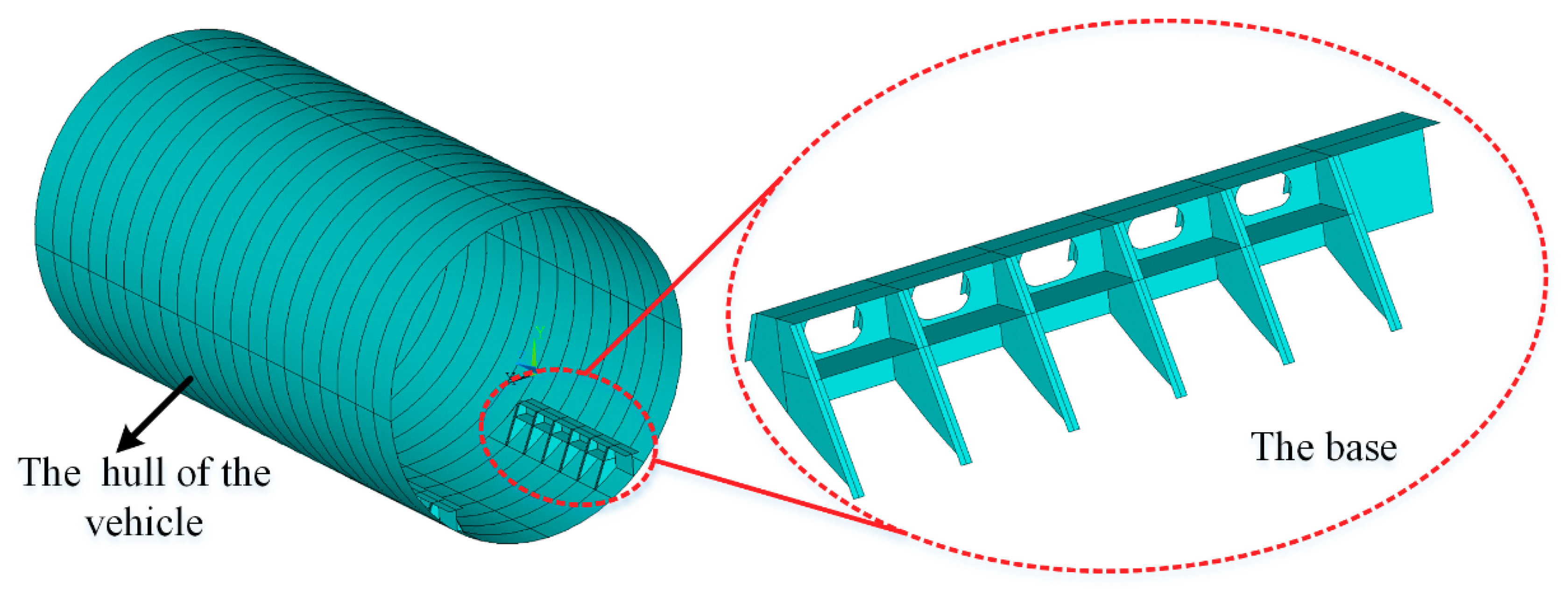
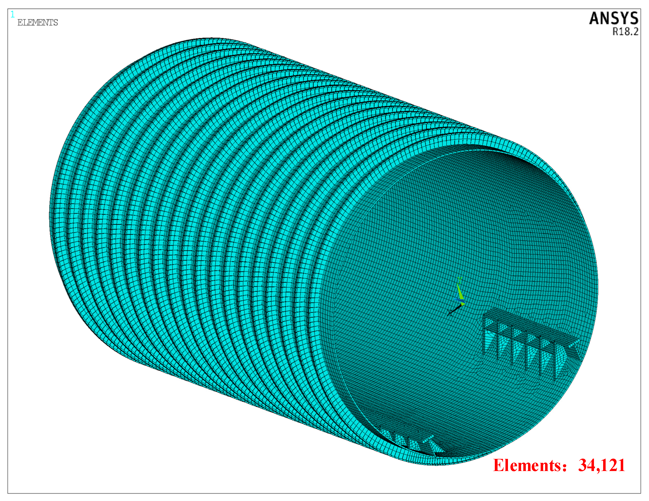
4.2. Engineering Application

In this section, an underwater vehicle base design problem is utilized to verify the effectiveness of the proposed method. The base is a braced structure for vibration devices in the hull of an underwater vehicle. The main capability of the base provides a platform for the installation of some imported vibration equipment and avoids the vibration transmitting to the hull directly. Meanwhile, the mechanical impedance of the base has a determination effect in reducing the level of noise. Specifically, the mechanical impedance is expected at a high level under all computational frequencies. The structural profile of the base adjoined to the hull of the underwater vehicle is depicted in Figure 6. The fixed structural and material parameters of the cylindrical shell and the base are listed in

Table 7. The values of the fixed structural and material parameters.

Fixed Parameters	Values
Elastic modulus $E$	$2.09\times {10}^5 \mathrm{MPa}$
Density $\rho$	$7850 \mathrm{kg}/{\mathrm{m}}^3$
Poisson’s ratio $\mu$	0.3
The length of the Hull $L$	12,000 mm
The radius of the Hull $R$	3300 mm
Rib space $l$	600 mm
Size of the ribs’	$14\times 224/26\times 80$ mm
The radius of the base web opening $r$	75 mm
Width of the base web opening $d$	210 mm

.

In this work, the objective is to maximize the minimum difference of the impedance between the scheme in design and the required impedance value under the same frequency. Simultaneously, the weight of the optimized scheme should be less than that of the allowable one. Therefore, the optimization problem can be described as,

$$\begin{array}{l}find\hspace{1em}\mathit{x}=\left[x_1,\dots ,x_6\right]\\ \max f(\mathit{x})=\min \left\{I(\mathit{x},{\omega }_i)-I({\mathit{x}}_0,{\omega }_i);i=1,2,\dots ,k\right\}\\ s.t. g(\mathit{x})=W(\mathit{x})-W({\mathit{x}}_0)<0\end{array}$$

(38)

where $\mathit{x}$ represents the vector of the design variables, which is a six-dimensional vector.${\omega }_i$ is the i^th computational frequency. In detail, the design variables of this problem are the thickness of the panels of the base. Figure 7 plots the schematic diagram and

Table 8. The meaning and ranges of the design variables.

Design Variables		Ranges
Former half	The thickness of the base panel $t_1$	40–90 mm
	The thickness of the base web $t_3$	10–60 mm
	The thickness of the base bracket $t_5$	12–40 mm
Remaining half	The thickness of the base panel $t_2$	40–90 mm
	The thickness of the base web $t_4$	10–60 mm
	The thickness of the base bracket $t_6$	12–40 mm

lists the meanings and value space of the design variables, respectively. $I(\mathit{x},{\omega }_i)$ and $W(\mathit{x})$ represent the impedance value under a specific computational frequency and the weight of the base, respectively.$I(\mathit{x},{\omega }_i)$ and $W({\mathit{x}}_0)$ are the required impedance value at the i^th computational frequency and the allowable base weight, respectively.

Generally, the responses of the impedance curve are obtained through the finite element simulation software ANSYS 18.1. The computational platform is with a 4.01 GHz Intel(R) Eight-Core (TM) i9-9900ks Processor and 64 GB RAM. In this simulation, the boundary condition is fixed for all the translation degrees at both sides of the shell. The loading is a unit vertical force at point A as depicted in Figure 7. The ribs are simulated by the Beam 188 element and the rest of the model is simulated by the Shell 181 element. The number of elements has to be more than 34,000 to get a desirable accuracy of the impedance value, as shown in Figure 8. Then, the frequency step is set to be 2.5 Hz and the computational frequency ranges from 0 to 350 Hz. To improve the efficiency of the optimization, minimal convex polygon technology is adopted to pre-process the impedance curve. In that case, the global feature of the curve and the minimum impedance value of the impedance curve are preserved. However, these complex and multimodal features, which may disturb the convergence speed of the optimization process, are filtered. Figure 9 illustrates the impedance curves before and after pre-processing on the scheme $\mathit{x}=\left[60,60,30,30,24,24\right]$.

As shown in Figure 9, the red line denotes the real impedance curve, which fluctuates significantly under different frequencies. The black line is the impedance curve after the pre- processing operation, which is smooth and the minimum value of the original curve remains the same. The blue line is the required impedance curve under different frequencies. Moreover, the allowance weight for this case is 3.027t and the maximum iteration of this case is set to be 50. To eliminate the randomness of the initial samples and the genetic algorithm, all methods use the same 60 initial LHS samples and the same setups of the genetic algorithm. Moreover, all the methods are repeated 20 times to avoid randomness occurring even though the setups are the same. The statistical optimization results of this problem with all compared methods of under 20 runs are summarized in

Table 9. The statistical optimization results of the engineering case with different methods.

Methods	$\mathit{f}(\mathit{x})\mathbf{(}\times {\mathbf{10}}^{\mathbf{5}}\mathbf{Ns}/\mathbf{m})$
	Max	Mean	Std	Succeeded
EI	4.031	3.998	0.03060	20/20
WEI	4.042	3.983	0.04316	20/20
LCB	3.857	3.733	0.08629	5/20
PLCB	3.892	3.723	0.12230	11/20
EW-LCB	4.062	4.027	0.01953	20/20

. Furthermore, the detailed design variables, optimal, and weights of all runs are listed in

Table A1. Detailed optimization results of the engineering case with different methods.

Methods	Variables (Rounded)						$\begin{array}{c}\mathit{f}(\mathit{x})\\ \mathbf{(}\times {\mathbf{10}}^{\mathbf{5}}\mathbf{Ns}/\mathbf{m})\end{array}$	Weight (t)
	t1 mm	t3 mm	t5 mm	t2 mm	t4 mm	t6 mm		Allowance 3.0327
EI	88	59	12	40	16	12	3.945	3.0058
	90	60	12	40	13	13	3.991	3.0151
	90	60	12	40	14	12	4.020	3.0136
	90	59	12	40	15	12	4.031	3.0125
	83	60	12	40	20	12	4.004	3.0158
	88	59	12	40	16	12	3.945	3.0058
	90	60	12	40	13	13	3.991	3.0151
	90	60	12	40	14	12	4.020	3.0136
	90	59	12	40	15	12	4.031	3.0125
	83	60	12	40	20	12	4.004	3.0158
	88	59	12	40	16	12	3.945	3.0058
	90	60	12	40	13	13	3.991	3.0151
	90	60	12	40	14	12	4.020	3.0136
	90	59	12	40	15	12	4.031	3.0125
	83	60	12	40	20	12	4.004	3.0158
	88	59	12	40	16	12	3.945	3.0058
	90	60	12	40	13	13	3.991	3.0151
	90	60	12	40	14	12	4.020	3.0136
	90	59	12	40	15	12	4.031	3.0125
	83	60	12	40	20	12	4.004	3.0158
WEI	88	59	12	40	16	13	3.919	3.0172
	89	60	12	40	14	12	4.042	3.0047
	88	60	12	40	16	12	4.013	3.0172
	83	60	13	40	20	12	3.974	3.0266
	82	60	13	40	21	12	3.964	3.0281
	88	59	12	40	16	13	3.919	3.0172
	89	60	12	40	14	12	4.042	3.0047
	88	60	12	40	16	12	4.013	3.0172
	82	60	13	40	21	12	3.964	3.0281
	83	60	13	40	20	12	3.974	3.0266
	88	59	12	40	16	13	3.919	3.0172
	89	60	12	40	14	12	4.042	3.0047
	88	60	12	40	16	12	4.013	3.0172
	83	60	13	40	20	12	3.974	3.0266
	82	60	13	40	21	12	3.964	3.0281
	88	59	12	40	16	13	3.919	3.0172
	89	60	12	40	14	12	4.042	3.0047
	88	60	12	40	16	12	4.013	3.0172
	83	60	13	40	20	12	3.974	3.0266
	82	60	13	40	21	12	3.964	3.0281
LCB	81	58	16	42	18	12	3.808	3.0203
	78	58	20	40	18	14	3.857	3.0457
	75	52	17	46	17	21	3.676	3.0409
	69	51	25	43	20	19	3.688	3.0617
	76	50	21	44	15	22	3.647	3.0499
	81	58	16	42	18	12	3.808	3.0203
	78	58	20	40	18	14	3.857	3.0457
	75	52	17	46	17	21	3.676	3.0409
	69	51	25	43	20	19	3.688	3.0617
	76	50	21	44	15	22	3.647	3.0499
	81	58	16	42	18	12	3.808	3.0203
	78	58	20	40	18	14	3.857	3.0457
	75	52	17	46	17	21	3.676	3.0409
	69	51	25	43	20	19	3.688	3.0617
	76	50	21	44	15	22	3.647	3.0499
	81	58	16	42	18	12	3.808	3.0203
	78	58	20	40	18	14	3.857	3.0457
	75	52	17	46	17	21	3.676	3.0409
	78	47	21	47	14	20	3.651	3.0303
	70	51	25	49	12	21	3.632	3.0461
PLCB	78	55	12	40	11	12	3.892	2.8243
	84	47	17	46	12	21	3.769	3.0154
	84	47	24	42	12	19	3.748	3.0331
	45	51	33	46	35	17	3.533	3.1076
	84	38	28	44	15	19	3.684	3.0270
	78	55	12	40	11	12	3.892	2.8243
	84	47	17	46	12	21	3.769	3.0154
	84	47	24	42	12	19	3.748	3.0331
	45	51	33	46	35	17	3.533	3.1076
	84	38	28	44	15	19	3.684	3.0270
	78	55	12	40	11	12	3.892	2.8243
	84	47	17	46	12	21	3.769	3.0154
	84	47	24	42	12	19	3.748	3.0331
	45	51	33	46	35	17	3.533	3.1076
	84	38	28	44	15	19	3.684	3.0270
	78	55	12	40	11	12	3.892	2.8243
	84	47	17	46	12	21	3.769	3.0154
	84	47	24	42	12	19	3.748	3.0331
	67	59	39	40	11	12	3.645	3.0369
	45	51	35	47	33	16	3.524	3.1050
EW-LCB	88	60	12	40	15	12	4.015	3.0065
	87	60	12	40	17	12	4.017	3.0187
	87	60	12	40	17	12	4.016	3.0187
	85	60	12	40	18	12	4.016	3.0118
	84	60	12	40	18	12	4.015	3.0034
	88	60	12	40	15	12	4.015	3.0065
	87	60	12	40	17	12	4.017	3.0187
	87	60	12	40	17	12	4.016	3.0187
	85	60	12	40	18	12	4.016	3.0118
	84	60	12	40	18	12	4.015	3.0034
	88	60	12	40	15	12	4.015	3.0065
	87	60	12	40	17	12	4.017	3.0187
	87	60	12	40	17	12	4.016	3.0187
	85	60	12	40	18	12	4.016	3.0118
	84	60	12	40	18	12	4.015	3.0034
	89	59	12	40	16	12	4.061	3.0143
	89	58	12	40	16	12	4.056	3.0026
	88	60	12	40	16	12	4.062	3.0172
	89	60	12	40	14	12	4.060	3.0047
	89	60	12	40	15	12	4.059	3.0155

Note: the weights which are larger than the allowable ones are marked by red.

in the Appendix.

As illustrated in Table 9, the best value of the proposed method is $4.062\times {10}^{5}Nm/s$, which is the maximum optimal value among all methods. Moreover, the proposed method has the maximum mean value on the objective among all the listed methods. It indicates the effectiveness of the proposed approach. Regarding robustness, the proposed method also performs best among all these methods because the proposed method obtains the minimum standard deviation. It is worth mentioning that the LCB and PLCB methods obtain some infeasible solutions. In detail, there are 15 and 9 runs that have failed for the LCB and PLCB methods respectively. The results show that the proposed method is a stable and effective method to solve this engineering optimization problem. Figure 10 shows the impedance curves of the optimal scheme of the proposed approach and the original scheme. As illustrated in Figure 10, the impedance curve of the optimal scheme is better than that of the original scheme because the impedance curve has larger impedance values in the frequencies which are critical to the performance of the base as shown in the sub-figure of Figure 9. On the other side, in the frequencies which are not critical to the performance of the base, the optimal scheme has smaller values than those of the original scheme. Therefore, the proposed approach is an effective method for this engineering case.

5. Conclusions

To balance exploration and exploitation during the sequential process of the AKBDO, an EW- LCB approach was developed in this work to obtain an optimal solution with less computational resources. In the proposed EW-LCB approach, entropy theory was adopted to quantify the degree of variation of the predicted value and variance of the Kriging model, respectively. Then, the weights were assigned to the LCB function automatically according to the relative values of the entropy theory. Meanwhile, an index factor was defined, which changed with iterations of the appearance of the current optimum, to avoid the sequential process being lost in the local optimum. The updated point was generated by minimizing the EW-LCB function, and the Kriging model updated sequentially. To test the performance of the proposed EW-LCB methods, four typical AKBDO methods including EI, WEI, LCB, and PLCB were adopted for comparison on ten widely used benchmark numerical functions and an engineering case. Results show that the proposed EW-LCB approach can obtain the optimum with the desired accuracy using less computational burden. Moreover, the proposed method has competitive robustness compared with state-of-the-art methods.

It is of note that the proposed method can handle constrained optimization problems by transferring the constrained optimization to the unconstrained one using the penalty methods. In practical engineering cases, simulation models with different fidelities always are available, as part of our future work, the developed EW-LCB method will be extended to the multi-fidelity scenario.

References

1. Han, Z.; Xu, C.; Zhang, L.; Zhang, Y.; Zhang, K.; Song, W. Efficient aerodynamic shape optimization using variable-fidelity surrogate models and multilevel computational grids. Chin. J. Aeronaut. 2020, 33, 31–47. [Google Scholar] [CrossRef]
2. Zhou, Q.; Wu, J.; Xue, T.; Jin, P. A two-stage adaptive multi-fidelity surrogate model-assisted multi-objective genetic algorithm for computationally expensive problems. Eng. Comput. 2019, 1–17. [Google Scholar] [CrossRef]
3. Velayutham, K.; Venkadeshwaran, K.; Selvakumar, G. Process Parameter Optimization of Laser Forming Based on FEM-RSM-GA Integration Technique. Appl. Mech. Mater. 2016, 852, 236–240. [Google Scholar] [CrossRef]
4. Gutmann, H.M. A radial basis function method for global optimization. J. Glob. Optim. 2001, 19, 201–227. [Google Scholar] [CrossRef]
5. Zhou, Q.; Rong, Y.; Shao, X.; Jiang, P.; Gao, Z.; Cao, L. Optimization of laser brazing onto galvanized steel based on ensemble of metamodels. J. Intell. Manuf. 2018, 29, 1417–1431. [Google Scholar] [CrossRef]
6. Sacks, J.; Welch, W.J.; Mitchell, T.J.; Wynn, H.P. Design and analysis of computer experiments. Stat. Sci. 1989, 4, 409–423. [Google Scholar] [CrossRef]
7. Zhou, Q.; Wang, Y.; Choi, S.-K.; Jiang, P.; Shao, X.; Hu, J.; Shu, L. A robust optimization approach based on multi-fidelity metamodel. Struct. Multidiscip. Optim. 2018, 57, 775–797. [Google Scholar] [CrossRef]
8. Shu, L.; Jiang, P.; Song, X.; Zhou, Q. Novel Approach for Selecting Low-Fidelity Scale Factor in Multifidelity Metamodeling. AIAA J. 2019, 57, 5320–5330. [Google Scholar] [CrossRef]
9. Zhou, Q.; Shao, X.; Jiang, P.; Zhou, H.; Shu, L. An adaptive global variable fidelity metamodeling strategy using a support vector regression based scaling function. Simul. Model. Pract. Theory 2015, 59, 18–35. [Google Scholar] [CrossRef]
10. Jiang, C.; Cai, X.; Qiu, H.; Gao, L.; Li, P. A two-stage support vector regression assisted sequential sampling approach for global metamodeling. Struct. Multidiscip. Optim. 2018, 58, 1657–1672. [Google Scholar] [CrossRef]
11. Qian, J.; Yi, J.; Cheng, Y.; Liu, J.; Zhou, Q. A sequential constraints updating approach for Kriging surrogate model-assisted engineering optimization design problem. Eng. Comput. 2019, 36, 993–1009. [Google Scholar] [CrossRef]
12. Shishi, C.; Zhen, J.; Shuxing, Y.; Apley, D.W.; Wei, C. Nonhierarchical multi-model fusion using spatial random processes. Int. J. Numer. Methods Eng. 2016, 106, 503–526. [Google Scholar] [CrossRef]
13. Hennig, P.; Schuler, C.J. Entropy search for information-efficient global optimization. J. Mach. Learn. Res. 2012, 13, 1809–1837. [Google Scholar]
14. Forrester, A.I.J.; Sóbester, A.; Keane, A.J. Engineering Design via Surrogate Modelling: A Practical Guide; John Wiley and Sons: Hoboken, NJ, USA, 2008. [Google Scholar]
15. Shu, L.; Jiang, P.; Wan, L.; Zhou, Q.; Shao, X.; Zhang, Y. Metamodel-based design optimization employing a novel sequential sampling strategy. Eng. Comput. 2017, 34, 2547–2564. [Google Scholar] [CrossRef]
16. Zhou, Q.; Wang, Y.; Choi, S.-K.; Jiang, P.; Shao, X.; Hu, J. A sequential multi-fidelity metamodeling approach for data regression. Knowl.-Based Syst. 2017, 134, 199–212. [Google Scholar] [CrossRef]
17. Dong, H.; Song, B.; Dong, Z.; Wang, P. SCGOSR: Surrogate-based constrained global optimization using space reduction. Appl. Soft Comput. 2018, 65, 462–477. [Google Scholar] [CrossRef]
18. Dong, H.; Song, B.; Dong, Z.; Wang, P. Multi-start Space Reduction (MSSR) surrogate-based global optimization method. Struct. Multidiscip. Optim. 2016, 54, 907–926. [Google Scholar] [CrossRef]
19. Serani, A.; Pellegrini, R.; Wackers, J.; Jeanson, C.-E.; Queutey, P.; Visonneau, M.; Diez, M. Adaptive multi-fidelity sampling for CFD-based optimisation via radial basis function metamodels. Int. J. Comput. Fluid Dyn. 2019, 33, 237–255. [Google Scholar] [CrossRef]
20. Pellegrini, R.; Iemma, U.; Leotardi, C.; Campana, E.F.; Diez, M. Multi-fidelity adaptive global metamodel of expensive computer simulations. In Proceedings of the 2016 IEEE Congress on Evolutionary Computation (CEC), Vancouver, BC, Canada, 24–29 July 2016; pp. 4444–4451. [Google Scholar]
21. Jones, D.; Schonlau, M.; Welch, W. Efficient global optimization of expensive black-box functions. J. Glob. Optim. 1998, 13, 455–492. [Google Scholar] [CrossRef]
22. Cox, D.D.; John, S. A statistical method for global optimization. In Proceedings of the 1992 IEEE International Conference on Systems, Man, and Cybernetics, Chicago, IL, USA, 18–21 October 1992; Volume 1242, pp. 1241–1246. [Google Scholar]
23. Li, G.; Zhang, Q.; Sun, J.; Han, Z. Radial basis function assisted optimization method with batch infill sampling criterion for expensive optimization. In Proceedings of the 2019 IEEE Congress on Evolutionary Computation (CEC), Wellington, New Zealand, 10–13 June 2019; pp. 1664–1671. [Google Scholar]
24. Diez, M.; Volpi, S.; Serani, A.; Stern, F.; Campana, E.F. Simulation-based design optimization by sequential multi-criterion adaptive sampling and dynamic radial basis functions. In Advances in Evolutionary and Deterministic Methods for Design, Optimization and Control in Engineering and Sciences; Springer: Berlin/Heidelberg, Germany, 2019; pp. 213–228. [Google Scholar]
25. Boukouvala, F.; Ierapetritou, M.G. Derivative-free optimization for expensive constrained problems using a novel expected improvement objective function. AIChE J. 2014, 60, 2462–2474. [Google Scholar] [CrossRef]
26. Li, Z.; Wang, X.; Ruan, S.; Li, Z.; Shen, C.; Zeng, Y. A modified hypervolume based expected improvement for multi-objective efficient global optimization method. Struct. Multidiscip. Optim. 2018, 58, 1961–1979. [Google Scholar] [CrossRef]
27. Li, L.; Wang, Y.; Trautmann, H.; Jing, N.; Emmerich, M. Multiobjective evolutionary algorithms based on target region preferences. Swarm Evol. Comput. 2018, 40, 196–215. [Google Scholar] [CrossRef]
28. Xiao, S.; Rotaru, M.; Sykulski, J.K. Adaptive Weighted Expected Improvement With Rewards Approach in Kriging Assisted Electromagnetic Design. IEEE Trans. Magn. 2013, 49, 2057–2060. [Google Scholar] [CrossRef] [Green Version]
29. Zhan, D.; Cheng, Y.; Liu, J. Expected improvement matrix-based infill criteria for expensive multiobjective optimization. IEEE Trans. Evol. Comput. 2017, 21, 956–975. [Google Scholar] [CrossRef]
30. Sasena, M.J. Flexibility and Efficiency Enhancements for Constrained Global Design Optimization with Kriging Approximations. Ph.D. Thesis, University of Michigan, Ann Arbor, MI, USA, 2002. [Google Scholar]
31. Forrester, A.I.J.; Keane, A.J. Recent advances in surrogate-based optimization. Prog. Aerosp. Sci. 2009, 45, 50–79. [Google Scholar] [CrossRef]
32. Zheng, J.; Li, Z.; Gao, L.; Jiang, G. A parameterized lower confidence bounding scheme for adaptive metamodel-based design optimization. Eng. Comput. 2016, 33, 2165–2184. [Google Scholar] [CrossRef]
33. Cheng, J.; Jiang, P.; Zhou, Q.; Hu, J.; Yu, T.; Shu, L.; Shao, X. A lower confidence bounding approach based on the coefficient of variation for expensive global design optimization. Eng. Comput. 2019, 36, 1–21. [Google Scholar] [CrossRef]
34. Srinivas, N.; Krause, A.; Kakade, S.M.; Seeger, M.W. Information-Theoretic Regret Bounds for Gaussian Process Optimization in the Bandit Setting. IEEE Trans. Inf. Theory 2012, 58, 3250–3265. [Google Scholar] [CrossRef] [Green Version]
35. Desautels, T.; Krause, A.; Burdick, J.W. Parallelizing exploration-exploitation tradeoffs in Gaussian process bandit optimization. J. Mach. Learn. Res. 2014, 15, 3873–3923. [Google Scholar]
36. Yondo, R.; Andrés, E.; Valero, E. A review on design of experiments and surrogate models in aircraft real-time and many-query aerodynamic analyses. Prog. Aerosp. Sci. 2018, 96, 23–61. [Google Scholar] [CrossRef]
37. Candelieri, A.; Perego, R.; Archetti, F. Bayesian optimization of pump operations in water distribution systems. J. Glob. Optim. 2018, 71, 213–235. [Google Scholar] [CrossRef] [Green Version]
38. Krige, D.G. A statistical approach to some basic mine valuation problems on the witwatersrand. J. South. Afr. Inst. Min. Metall. 1952, 52, 119–139. [Google Scholar]
39. Guo, Z.; Song, L.; Park, C.; Li, J.; Haftka, R.T. Analysis of dataset selection for multi-fidelity surrogates for a turbine problem. Struct. Multidiscip. Optim. 2018, 57, 2127–2142. [Google Scholar] [CrossRef]
40. Deb, K. An efficient constraint handling method for genetic algorithms. Comput. Methods Appl. Mech. Eng. 2000, 186, 311–338. [Google Scholar] [CrossRef]
41. Schutte, J.F.; Reinbolt, J.A.; Fregly, B.J.; Haftka, R.T.; George, A.D. Parallel global optimization with the particle swarm algorithm. Int. J. Numer. Methods Eng. 2004, 61, 2296–2315. [Google Scholar] [CrossRef] [PubMed] [Green Version]
42. Volpi, S.; Diez, M.; Gaul, N.J.; Song, H.; Iemma, U.; Choi, K.; Campana, E.F.; Stern, F. Development and validation of a dynamic metamodel based on stochastic radial basis functions and uncertainty quantification. Struct. Multidiscip. Optim. 2015, 51, 347–368. [Google Scholar] [CrossRef]
43. Liu, J.; Han, Z.; Song, W. Comparison of infill sampling criteria in kriging-based aerodynamic optimization. In Proceedings of the 28th Congress of the International Council of the Aeronautical Sciences, Brisbane, Australia, 23–28 September 2012; pp. 23–28. [Google Scholar]
44. Loeppky, J.L.; Sacks, J.; Welch, W.J. Choosing the sample size of a computer experiment: A practical guide. Technometrics 2009, 51, 366–376. [Google Scholar] [CrossRef] [Green Version]
45. Jin, R.; Chen, W.; Sudjianto, A. An efficient algorithm for constructing optimal design of computer experiments. J. Stat. Plan. Inference 2005, 134, 268–287. [Google Scholar] [CrossRef]
46. Lophaven, S.N.; Nielsen, H.B.; Søndergaard, J. DACE: A Matlab Kriging Toolbox, Version 2.0; Technical Report Informatics and Mathematical Modelling, (IMM-TR)(12); Technical University of Denmark: Lyngby, Denmark, 2002; pp. 1–34. [Google Scholar]
47. Homaifar, A.; Qi, C.X.; Lai, S.H. Constrained optimization via genetic algorithms. Simulation 1994, 62, 242–253. [Google Scholar] [CrossRef]
48. Gadre, S.R. Information entropy and Thomas-Fermi theory. Phys. Rev. A 1984, 30, 620. [Google Scholar] [CrossRef]
49. de Boer, P.-T.; Kroese, D.P.; Mannor, S.; Rubinstein, R.Y. A Tutorial on the Cross-Entropy Method. Ann. Oper. Res. 2005, 134, 19–67. [Google Scholar] [CrossRef]
50. Jiang, P.; Cheng, J.; Zhou, Q.; Shu, L.; Hu, J. Variable-Fidelity Lower Confidence Bounding Approach for Engineering Optimization Problems with Expensive Simulations. AIAA J. 2019, 57, 5416–5430. [Google Scholar] [CrossRef]
51. Zhou, Q.; Shao, X.Y.; Jiang, P.; Gao, Z.M.; Zhou, H.; Shu, L.S. An active learning variable-fidelity metamodelling approach based on ensemble of metamodels and objective-oriented sequential sampling. J. Eng. Des. 2016, 27, 205–231. [Google Scholar] [CrossRef]
52. Toal, D.J.J. Some considerations regarding the use of multi-fidelity Kriging in the construction of surrogate models. Struct. Multidiscip. Optim. 2015, 51, 1223–1245. [Google Scholar] [CrossRef] [Green Version]
53. Jiao, R.; Zeng, S.; Li, C.; Jiang, Y.; Jin, Y. A complete expected improvement criterion for Gaussian process assisted highly constrained expensive optimization. Inf. Sci. 2019, 471, 80–96. [Google Scholar] [CrossRef]
54. Bali, K.K.; Gupta, A.; Ong, Y.S.; Tan, P.S. Cognizant Multitasking in Multiobjective Multifactorial Evolution: MO-MFEA-II. IEEE Trans. Cybern. 2020, 1–13. [Google Scholar] [CrossRef]
55. Pellegrini, R.; Serani, A.; Liuzzi, G.; Rinaldi, F.; Lucidi, S.; Campana, E.F.; Iemma, U.; Diez, M. Hybrid Global/Local Derivative-Free Multi-objective Optimization via Deterministic Particle Swarm with Local Linesearch. In Proceedings of the Machine Learning, Optimization, and Big Data, Third International Conference, MOD 2017, Cham, Switzerland, 14–17 September 2017; pp. 198–209. [Google Scholar]
56. Pellegrini, R.; Serani, A.; Leotardi, C.; Iemma, U.; Campana, E.F.; Diez, M. Formulation and parameter selection of multi-objective deterministic particle swarm for simulation-based optimization. Appl. Soft Comput. 2017, 58, 714–731. [Google Scholar] [CrossRef]
57. Zhang, T.; Yang, C.; Chen, H.; Sun, L.; Deng, K. Multi-objective optimization operation of the green energy island based on Hammersley sequence sampling. Energy Convers. Manag. 2020, 204, 112316. [Google Scholar] [CrossRef]
58. Zheng, J.; Shao, X.; Gao, L.; Jiang, P.; Qiu, H. A prior-knowledge input LSSVR metamodeling method with tuning based on cellular particle swarm optimization for engineering design. Expert Syst. Appl. 2014, 41, 2111–2125. [Google Scholar] [CrossRef]
59. Garcia, S.; Herrera, F. An extension on “statistical comparisons of classifiers over multiple data sets” for all pairwise comparisons. J. Mach. Learn. Res. 2008, 9, 2677–2694. [Google Scholar]
Figure 1. The framework of the proposed entropy weight algorithm (EW-LCB).
Applsci 10 03554 g001
Figure 2. The initial Kriging model of the illustrated example.
Applsci 10 03554 g002
Figure 3. The first iteration of the proposed approach with the illustrated function.
Applsci 10 03554 g003
Figure 4. The final result of the proposed approach on the illustrated function.
Applsci 10 03554 g004
Figure 5. The box plot of the FEmean with different methods.
Applsci 10 03554 g005
Figure 6. The structural profile of the base.
Applsci 10 03554 g006
Figure 7. The design variables and loads of the underwater vehicle base.
Applsci 10 03554 g007
Figure 8. The mesh model of the base with the shell of the underwater vehicle.
Applsci 10 03554 g008
Figure 9. The impedance curves before and after pre-processing.
Applsci 10 03554 g009
Figure 10. The impedance curve of the optimization solution.
Applsci 10 03554 g010