Trajectory Linearization-Based Adaptive PLOS Path Following Control for Unmanned Surface Vehicle with Unknown Dynamics and Rudder Saturation

Abstract

This paper presents a novel robust control strategy for path following of an unmanned surface vehicle (USV) suffering from unknown dynamics and rudder saturation. The trajectory linearization control (TLC) method augmented by the neural network, linear extended state observer (LESO), and auxiliary system is used as the main control framework. The salient features of the presented strategy are as follows: in the guidance loop, a fuzzy predictor line-of-sight (FPLOS) guidance law is proposed to ensure that the USV effectively follows the given path, where the fuzzy method is introduced to adjust lookahead distance online, and thereby achieving convergence performance; in the control loop, we develop a practical robust path following controller based on enhanced TLC, in which the neural network and LESO are adopted to handle unmodeled dynamics and external disturbances, respectively. Meanwhile, a nonlinear tracking differentiator (NTD) is constructed to achieve satisfactory differential and filter performance. Then, the auxiliary system is incorporated into the controller design to handle rudder saturation. Using Lyapunov stability theory, the entire system is ensured to be uniformly ultimately bounded (UUB). Simulation comparisons illustrate the effectiveness and superiority of the proposed strategy.

1. Introduction

In recent years, unmanned surface vehicles (USV) have received significant attention, due to their broad applications in the marine environment, such as ocean surveillance, gas exploration, and marine transportation [1,2,3]. In these applications, the high tracking performance and complex external environment make the USV path following control challenging.

Path following is a motion control scenario where the USV has to follow a predefined path without a temporal constraint [4,5,6]. At present, various control methods have been proposed in the literature. In [7], an adaptive control approach based on the backstepping technique was developed for an unmanned marine surface vessel, which was also suitable for other unmanned vehicles. Using the dynamic surface control (DSC) method, a practical path following control scheme was developed for underactuated ships in [8], whose advantage was that it could deal with the practical condition “waypoints based navigation”. The paper [9] presented an effective control approach for path following of marine vehicles, where the input-output feedback linearization method being applied by defining “hand position” as the output. In addition, a popular and effective guidance method adopted in path following is line-of-sight (LOS) guidance [10,11,12,13]. The main idea is to implement a lookahead based LOS guidance law mimicking a helmsman and generate a desired heading angle, which is fed into the inner dynamics loop. In [14], an integral LOS (ILOS) guidance law based on monotone cubic Hermite interpolation was developed, and the main innovation was that it proposed a time-varying equation for the lookahead distance. In [15], a novel guidance control method was presented for a marine surface vehicle (MSV), in which the unknown sideslip angle was estimated using a reduced-order ESO. The paper [16] proposed a sideslip-tangent LOS (SLOS) guidance strategy, where the sideslip angle was eliminated by constructing a finite-time sideslip observer (FSO). Compared with [14,15], the advantage was that it could handle a large sideslip angle. The paper [17] proposed an adaptive LOS (ALOS) algorithm for unmanned aerial vehicles, in which an adaptive law was constructed to handle the unknown sideslip angle.

On the other hand, in order to deal with complex interference, scholars have put forward many excellent solutions [18,19]. A concise path following controller was designed for a podded propulsion USV in [20], in which unmodeled dynamics and disturbances were handled by introducing the neural network minimum parameter learning method. The paper [21] proposed a robust compound control method subject to bounded uncertainties, where LESO was used to estimate the system uncertainties. A novel sigmoid function based disturbance observer was designed to eliminate various uncertainties effectively in [22], which was proven to be an efficient observer. The paper [23] developed an online constructive fuzzy approximator by the decoupled structure learning mechanism, which was incorporated into the dominant adaptive controller to identify unknown nonlinearities and unknown external disturbances exactly. Besides, input saturation [24,25] is common and inevitable, which may lead to system instability. In [26], a path following controller was presented for a surface vessel, in which the auxiliary system developed could cope very well with input saturation without any downtime. Considering disturbances and input saturation, the paper [27] addressed the course tracking problem of ships, where the rudder saturation was compensated using an auxiliary dynamic system. The paper [28] developed a novel trajectory tracking control method, in which a Gaussian error function was introduced to approximate input saturation.

Motivated by the above observations, considering unknown dynamics, disturbances, and rudder saturation, this article presents a novel path following control strategy for the USV. This paper covers the following three contributions:

(1)

An improved PLOS guidance law is constructed to calculate the desired heading angle and estimate unknown sideslip angle. Compared with [13], a fuzzy method is incorporated into the proposed PLOS guidance law to optimize the lookahead distance, thus achieving better convergence quality.

(2)

As a new control method in the USV motion control field, an enhanced TLC is adopted to design a concise path following controller for USV. Compared with traditional TLC, the enhanced TLC only needs one parameter to be adjusted.

(3)

Both unknown dynamics and disturbances can be estimated by constructing a neural network and LESO, respectively, and the rudder saturation is effectively resolved by using an auxiliary system.

The structure of this paper is as follows. The problem formulation and preliminaries are introduced in Section 2. Section 3 presents a novel control strategy for the USV. Stability analysis is given in Section 4. Section 5 is the simulation result verification. Finally, Section 6 gives the conclusions and future works.

2. Problem Formulation and Preliminaries

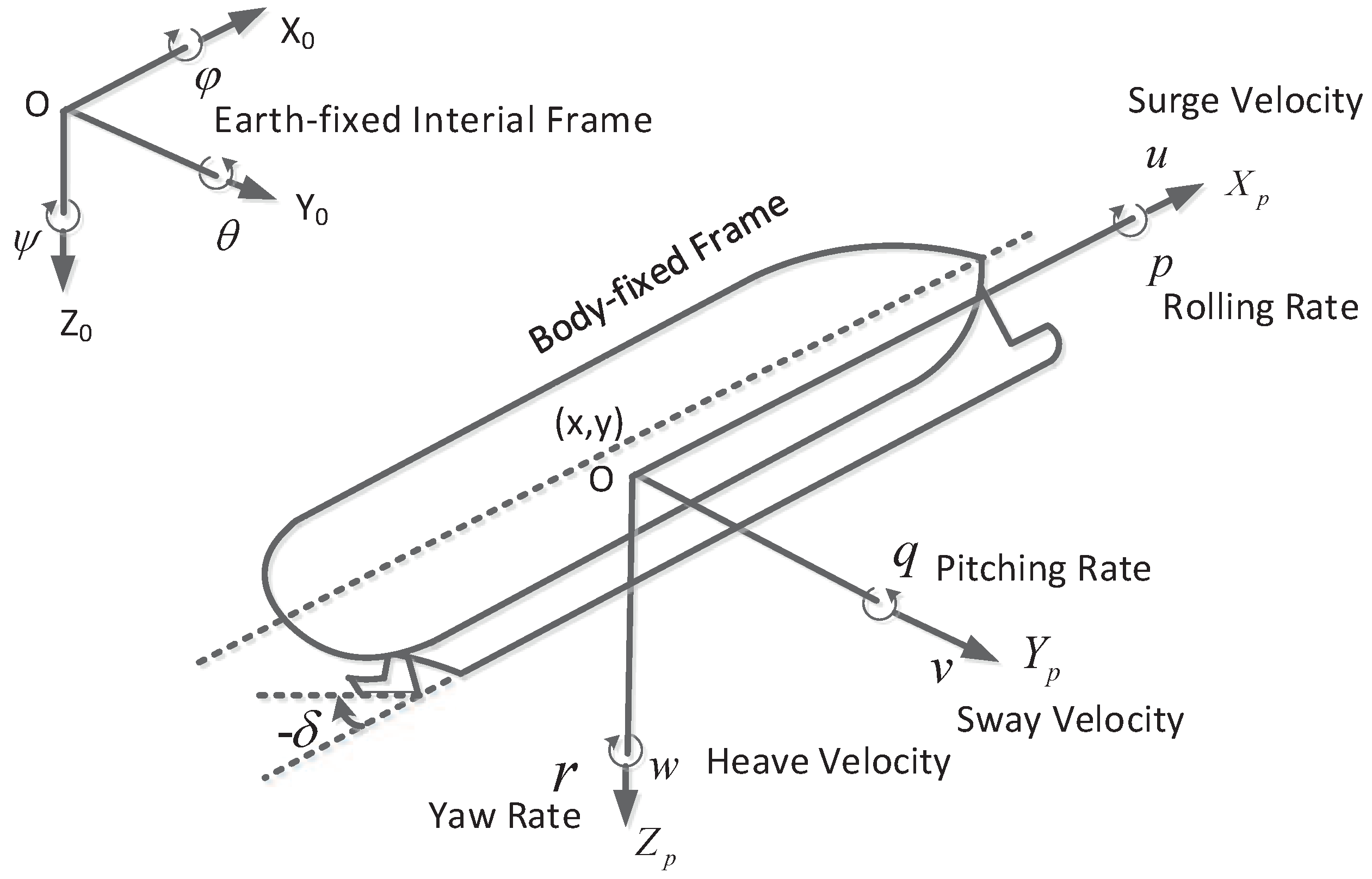
Notations: $\left|•\right|$ represents the absolute operator. $∥•∥$ represents the Euclidean norm. $\widehat{•}$ denotes the estimate value. $\widetilde{•}=\widehat{•}-•$ denotes the error.

2.1. USV Model

In this section, we first define the frames: the Earth-fixed inertial frame $X_{0}O{Y}_0$$\left(i\right)$ and the body-fixed frame $X_{p}O{Y}_p$$\left(b\right)$, as illustrated in Figure 1. Then, we only consider the horizontal motion of the USV, namely, neglecting roll p, pitch q, and heave w.

From [17], the kinematic equation of the USV can be modeled by:

$$\left\{\begin{array}{c}\dot{x}=ucos\psi -vsin\psi \hfill \\ \dot{y}=usin\psi +vcos\psi \hfill \\ \dot{\psi }=r\hfill \end{array}\right.$$

(1)

where $\left(x,y,\psi \right)$ is the position and orientation of the USV in $\left(i\right)$ and u, v, and r include the frame $\left(b\right)$ surge, sway, and yaw velocities, respectively.

Considering the actual situation of USV navigation, the Norrbin nonlinear model [27] with respect to USV steering control is given by:

$$\left\{\begin{array}{c}\dot{\psi }=r\hfill \\ \dot{r}=-\frac{1}{T}r-\frac{\alpha }{T}{r}^3+\frac{K}{T}\delta \hfill \end{array}\right.$$

(2)

where $\delta$ is the rudder angle, $\alpha$ is the Norrbin coefficient, T is the time constant, and K is the gain constant.

Combining the system (1) and (2), the nonlinear mathematical model of the USV is written as:

$$\left\{\begin{array}{c}\dot{x}=ucos\psi -vsin\psi \hfill \\ \dot{y}=usin\psi +vcos\psi \hfill \\ \dot{\psi }=r\hfill \\ \dot{r}=f\left(r\right)+\Delta f\left(r\right)+b\mu +d\hfill \\ y_1=x\hfill \\ y_2=y\hfill \end{array}\right.$$

(3)

where $f\left(r\right)=-\frac{1}{T}r-\frac{\alpha }{T}{r}^3$, $b=\frac{K}{T}$, and $y_1$, $y_2$ denote the output signal; $\Delta f\left(r\right)$, d represent unknown dynamics and multiple disturbances, respectively. $\mu =\delta$ is the input of the USV. Considering the saturation characteristics of the rudder, it can be described as:

$$\begin{array}{c}\hfill \mu =\left\{\begin{array}{c}{\mu }_{max},if{\mu }_0>{\mu }_{max}\hfill \\ {\mu }_0,if{\mu }_{min}\le {\mu }_0\le {\mu }_{max}\hfill \\ {\mu }_{min},if{\mu }_0<{\mu }_{min}\hfill \end{array}\right.\end{array}$$

(4)

where ${\mu }_{max}$ and ${\mu }_{min}$ represent the amplitudes of input saturation. From [29], we know ${\mu }_{max}={35}^{\circ }$, ${\mu }_{min}=-{35}^{\circ }$.

Remark 1.

Here, the frequency of d is low compared to the USV dynamics, and it is also filtered by a nonlinear tracking differentiator. Hence, d is considered to be slow time-varying disturbance [30].

Our control objective is to design a robust adaptive path following control strategy with completely unknown dynamics, disturbances, and rudder saturation, so that the USV tracks the reference path $\left(x_d,y_d\right)$ with an arbitrarily small error.

2.2. Preliminaries

Assumption 1.

The multiple disturbances are bounded with $\left|d\right|\le d_{max}$, where $d_{max}$ is unknown positive constant.

Lemma 1

([31]). Considering following system:

$$\begin{array}{c}\hfill \dot{X}=A_c\left(t\right)X\end{array}$$

(5)

where $A_c$ is continuous and bounded. Let $Q_l\left(t\right)$ be a bounded, positive, symmetric matrix, such as $0<{\lambda }_{3}I\le Q\left(t\right)\le {\lambda }_{4}I$. There exists a symmetric matrix $P\left(t\right)$ meeting:

$$\begin{array}{c}\hfill A_c^T\left(t\right)P\left(t\right)+P\left(t\right)A_c\left(t\right)+\dot{P}\left(t\right)+Q\left(t\right)=0\end{array}$$

(6)

where $P\left(t\right)={\int }_t^{\infty }{\hslash }^T\left(\iota ,t\right)Q\left(t\right)\hslash \left(\iota ,t\right)d\iota$, $∥\hslash \left(\iota ,t\right)∥\le o_1{e}^{-o_2\left(t-t_0\right)}$, $0<{\lambda }_{1}I\le P\left(t\right)\le {\lambda }_{2}I$.

Trajectory linearization control (TLC) [32,33,34,35]: TLC has proven to be an effective robust control method, whose structure is shown in Figure 2. It is clearly noticed that TLC consists of an open-loop dynamic inversion and a linear time-varying (LTV) feedback regulator, in which the dynamic inversion transforms the tracking problem into a time-varying nonlinear tracking error adjustment problem, and the LTV regulator achieves robust stability and performance along the nominal trajectory. Hence, TLC produces robust stability and anti-interference ability, for which TLC has been widely applied to a model-scaled helicopter [33], a 6DOF aircraft [34], and a car-like ground vehicle [35]. However, TLC is rarely used in the control of a USV.

Neural network: For unknown continuous function $\Delta f\left(X\right)$ (${\mathbb{R}}^m\to \mathbb{R}$), it can be approximated over a compact set ${\mathsf{\Phi }}_X\subseteq {\mathbb{R}}^m$ with the following radial basis function neural network (RBFNN):

$$\begin{array}{c}\hfill \Delta f\left(X\right)=W^{*T}S\left(X\right)+\epsilon \end{array}$$

(7)

where $X\in {\mathsf{\Phi }}_X$ denotes the input, $W^{*}\in {\mathbb{R}}^l$ denotes the ideal weight, and l is the node number. From [36], we know that the number of NN nodes determines the approximation ability, and the ideal weight vector is written as:

$$\begin{array}{c}\hfill W^{*}=arg\underset{\widehat{W}}{min}\left\{\underset{X\in {\mathsf{\Psi }}_X}{sup}\left|\Delta f\left(X\right)-{\widehat{W}}^{T}S\left(X\right)\right|\right\}\end{array}$$

(8)

$S\left(X\right)={\left[S_1\left(X\right),...,S_l\left(X\right)\right]}^T$ represents the RBF vector, which is defined by:

$$\begin{array}{c}\hfill S_i\left(X\right)=exp\left(-\frac{{∥X-{\rho }_i∥}^2}{2h_i^2}\right),i=1,...,l\end{array}$$

(9)

where ${\rho }_i$ and $h_i$ are the center and spread, respectively, and the approximation error $\epsilon$ is bounded with $\left|\epsilon \right|\le \overline{\epsilon }$, where $\overline{\epsilon }$ is unknown positive constant.

3. Path Following Control Strategy

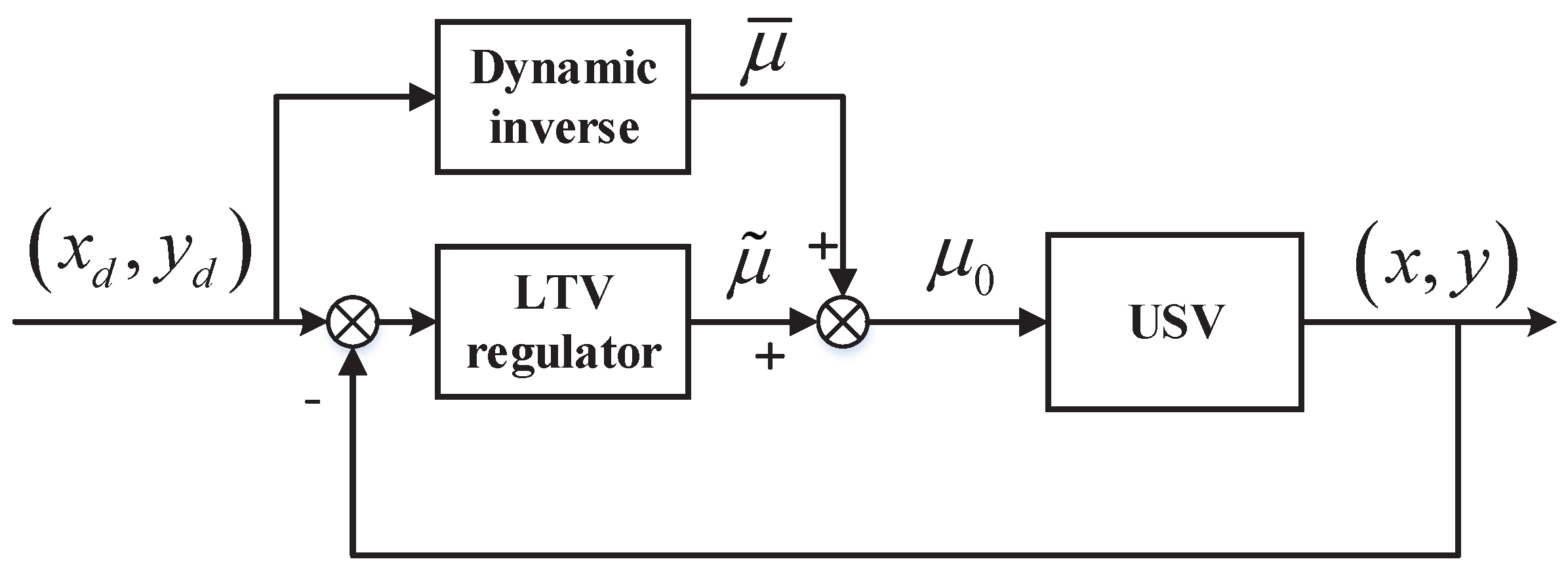
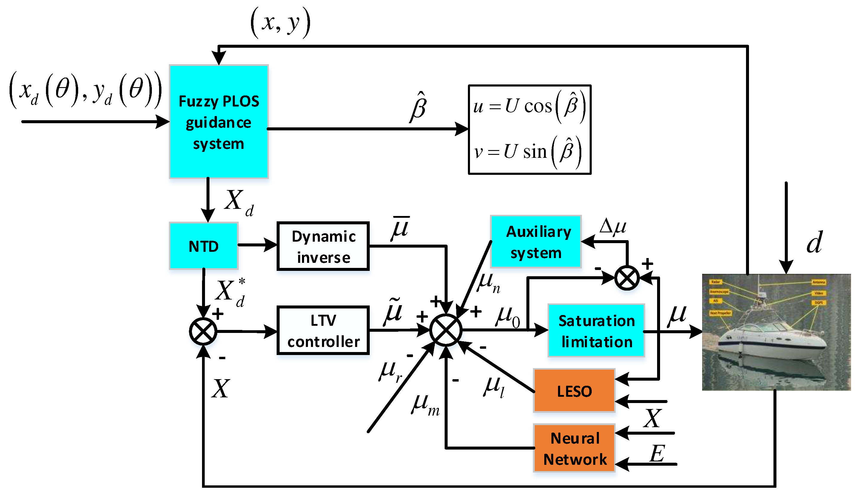
3.1. Structure of the Proposed Control Strategy

A novel path following control strategy is shown in Figure 3. We can see from Figure 3 that it consists mainly of the fuzzy predictor line-of-sight (FPLOS) guidance and the composite control strategy. The proposed FPLOS guidance strategy can not only provide the desired heading angle, but also compensate for the unknown sideslip angle. The proposed composite control strategy consists of two parts: the first part is that TLC controller ensures that the actual heading tracks the guidance heading; the second part is that the compensation controller is capable of solving unmodeled dynamics, multiple disturbances, and rudder saturation by using the NN, reduced-order LESO, and auxiliary system, respectively. Meanwhile, a nonlinear tracking differentiator (NTD) provides a satisfactory differentiation and filtering effect. In the control loop, ${\mu }_m$, ${\mu }_l$, and ${\mu }_n$ represent the outputs of NN, LESO, and auxiliary system, respectively; ${\mu }_r$ is a robust term.

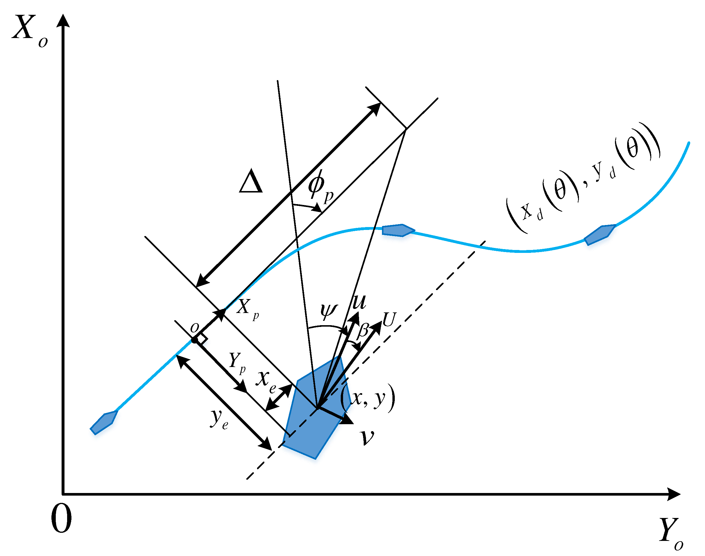
3.2. Guidance System Design

In this section, a predictor is used to estimate the unknown sideslip angle induced by wind, waves, and currents. Then, an FPLOS guidance law is proposed, where the lookahead distance is optimized using the fuzzy method.

3.2.1. Estimation of Sideslip Angle

As is illustrated in Figure 4, consider that the desired continuous path $\left(x_d\left(\theta \right),y_d\left(\theta \right)\right)$ to be tracked is parameterized by a path variable $\theta$. Then, the path-tangential angle ${\varphi }_p$ is given by:

$${\varphi }_p\left(\theta \right)=atan2\left({y^{\prime }}_d\left(\theta \right),{x^{\prime }}_d\left(\theta \right)\right)$$

(10)

where ${x^{\prime }}_d\left(\theta \right)=\partial x_d/\phantom{\partial x_d\partial \theta }\partial \theta$ and ${y^{\prime }}_d\left(\theta \right)=\partial y_d/\phantom{\partial y_d\partial \theta }\partial \theta$.

For the USV located at $\left(x,y\right)$, the errors $x_e$ and $y_e$ in $X_{p}o{Y}_p$ are written as:

$$\begin{array}{c}\hfill \left[\begin{array}{c}{x}_e\hfill \\ y_e\hfill \end{array}\right]={\left[\begin{array}{cc}cos{\varphi }_p& -sin{\varphi }_p\\ sin{\varphi }_p& cos{\varphi }_p\end{array}\right]}^T\left[\begin{array}{c}x-x_d\left(\theta \right)\\ y-y_d\left(\theta \right)\end{array}\right]\end{array}$$

(11)

where $y_e$ and $x_e$ denote cross- and along-track errors, respectively.

Calculating the derivative of (11) along (1) yields:

$$\begin{array}{cc}\hfill {\dot{x}}_e& =ucos\left(\psi -{\varphi }_p\right)-vsin\left(\psi -{\varphi }_p\right)\hfill \\ \hfill & +{\dot{\varphi }}_p\underset{y_e}{\underbrace{\left[-\left(x-x_d\right)sin{\varphi }_p+\left(y-y_d\right)cos{\varphi }_p\right]}}\hfill \\ \hfill & -\dot{\theta }\sqrt{{{x^{\prime }}_d}^2+{{y^{\prime }}_d}^2}cos\left({\varphi }_p+\phi \right)\hfill \\ \hfill & =Ucos\left(\psi -{\varphi }_p\right)cos\beta -Usin\left(\psi -{\varphi }_p\right)sin\beta \hfill \\ \hfill & +{\dot{\varphi }}_p{y}_e-u_p\hfill \\ \hfill {\dot{y}}_e& =usin\left(\psi -{\varphi }_p\right)+vcos\left(\psi -{\varphi }_p\right)\hfill \\ \hfill & -{\dot{\varphi }}_p\underset{x_e}{\underbrace{\left[-\left(x-x_d\right)cos{\varphi }_p+\left(y-y_d\right)sin{\varphi }_p\right]}}\hfill \\ \hfill & =Usin\left(\psi -{\varphi }_p\right)cos\beta +Ucos\left(\psi -{\varphi }_p\right)sin\beta \hfill \\ \hfill & -{\dot{\varphi }}_p{x}_e\hfill \end{array}$$

(12)

where $U=\sqrt{u^2+v^2}>0$, $0<U_{min}\le U\le U_{max}$, and $\beta =\mathrm{atan}2\left(v,u\right)$ denotes the sideslip angle. $u_p$ is the virtual target speed to stabilize $x_e$, which is selected as:

$$\begin{array}{c}\hfill u_p=\dot{\theta }\sqrt{{{x^{\prime }}_d}^2\left(\theta \right)+{{y^{\prime }}_d}^2\left(\theta \right)}\end{array}$$

(13)

Note that the sideslip angle is relatively small in practice [25], and we have:

$$\begin{array}{c}\hfill \left\{\begin{array}{c}{\dot{x}}_e=Ucos\left(\psi -{\varphi }_p\right)-Usin\left(\psi -{\varphi }_p\right)\beta +{\dot{\varphi }}_p{y}_e-u_p\hfill \\ {\dot{y}}_e=Usin\left(\psi -{\varphi }_p\right)+Ucos\left(\psi -{\varphi }_p\right)\beta -{\dot{\varphi }}_p{x}_e\hfill \end{array}\right.\end{array}$$

(14)

In order to exactly compensate for the unknown sideslip angle, two predictors are developed as:

$$\begin{array}{c}\hfill \left\{\begin{array}{c}{\dot{\widehat{x}}}_e=Ucos\left(\psi -{\varphi }_p\right)-Usin\left(\psi -{\varphi }_p\right)\widehat{\beta }+{\dot{\varphi }}_p{\widehat{y}}_e-u_p-k_x{\tilde{x}}_e\hfill \\ {\dot{\widehat{y}}}_e=Usin\left(\psi -{\varphi }_p\right)+Ucos\left(\psi -{\varphi }_p\right)\widehat{\beta }-{\dot{\varphi }}_p{\widehat{x}}_e-k_y{\tilde{y}}_e\hfill \end{array}\right.\end{array}$$

(15)

where $k_x$ and $k_y$ are the design parameters, ${\tilde{x}}_e={\widehat{x}}_e-x_e$, ${\tilde{y}}_e={\widehat{y}}_e-y_e$ are the prediction errors, and $\widehat{\beta }$ is the estimation of $\beta$. The corresponding adaptive updating law is selected as:

$$\begin{array}{c}\hfill \dot{\widehat{\beta }}=\gamma \left[Usin\left(\psi -{\varphi }_p\right){\tilde{x}}_e-Ucos\left(\psi -{\varphi }_p\right){\tilde{y}}_e\right]\end{array}$$

(16)

The,n ${\tilde{x}}_e$, ${\tilde{y}}_e$, and $\tilde{\beta }$ are written as:

$$\begin{array}{c}\hfill \left\{\begin{array}{c}{\dot{\tilde{x}}}_e=-Usin\left(\psi -{\varphi }_p\right)\tilde{\beta }-k_x{\tilde{x}}_e\hfill \\ {\dot{\tilde{y}}}_e=Ucos\left(\psi -{\varphi }_p\right)\tilde{\beta }-k_y\tilde{\beta }\hfill \\ \dot{\tilde{\beta }}=\gamma \left[Usin\left(\psi -{\varphi }_p\right){\tilde{x}}_e-Ucos\left(\psi -{\varphi }_p\right){\tilde{y}}_e\right]\hfill \end{array}\right.\end{array}$$

(17)

Theorem 1.

The proposed update law (16) makes the errors ${\tilde{x}}_e$ and ${\tilde{y}}_e$ to converge to origin, thus ensuring that the system (17) is uniformly asymptotically stable (UAS).

Proof of Theorem 1.

Define the Lyapunov function by:

$$\begin{array}{c}\hfill V_1=\frac{1}{2}{\tilde{x}}_e^2+\frac{1}{2}{\tilde{y}}_e^2+\frac{1}{2}{\gamma }^{-1}{\tilde{\beta }}^2\end{array}$$

(18)

Differentiating $V_1$ along (16) and (17) yields:

$$\begin{array}{cc}\hfill {\dot{V}}_1& ={\tilde{x}}_e\left(-Usin\left(\psi -{\varphi }_p\right)\tilde{\beta }-k_x{\tilde{x}}_e\right)+{\tilde{y}}_e\left(Ucos\left(\psi -{\varphi }_p\right)\tilde{\beta }-k_y\tilde{\beta }\right)\hfill \\ \hfill & +\tilde{\beta }\left(Usin\left(\psi -{\varphi }_p\right){\tilde{x}}_e-Ucos\left(\psi -{\varphi }_p\right){\tilde{y}}_e\right)\hfill \\ \hfill & \le -k_x{\tilde{x}}_e^2-k_y{\tilde{y}}_e^2\hfill \end{array}$$

(19)

Hence, we know that the system (17) is UAS. □

3.2.2. FPLOS Guidance Law

Then, the FPLOS guidance law is given by:

$$\begin{array}{c}\hfill {\psi }_d={\varphi }_p+arctan\left(-\frac{{\widehat{y}}_e}{\Delta }-\widehat{\beta }\right)\end{array}$$

(20)

where $\Delta$ is the user-specified lookahead distance.

Remark 2.

Different from the existing LOS guidance in [15,20], Δ of this paper changes with the movement of the USV. The greatest advantage of this proposed guidance strategy is to optimize Δ through the fuzzy method, thereby producing an aggressive behavior to decrease $y_e$ faster. Here, the inputs of the designed fuzzy system are $y_e$ and ${\dot{y}}_e$, and the output is Γ. the lookahead distance Δ is designed as $\Delta ={\Delta }_{min}+\mathsf{\Gamma }\left({\Delta }_{max}-{\Delta }_{min}\right)$.

The velocity $u_p$ is designed to stabilize $x_e$ as the virtual input, which is determined by:

$$\begin{array}{c}\hfill u_p=Ucos\left(\psi -{\varphi }_p\right)-Usin\left(\psi -{\varphi }_p\right)\widehat{\beta }+k_1{\widehat{x}}_e\end{array}$$

(21)

where $k_1$ denotes a positive constant.

From (13) and (21), the update law $\theta$ can be described by:

$$\begin{array}{c}\hfill \dot{\theta }=\frac{Ucos\left(\psi -{\varphi }_p\right)-Usin\left(\psi -{\varphi }_p\right)\widehat{\beta }+k_1{\widehat{x}}_e}{\sqrt{{{x^{\prime }}_d}^2\left(\theta \right)+{{y^{\prime }}_d}^2\left(\theta \right)}}\end{array}$$

(22)

Based on the above analysis, (15) can be rewritten as:

$$\begin{array}{c}\hfill \left\{\begin{array}{c}{\dot{\widehat{x}}}_e=-k_1{\widehat{x}}_e+{\dot{\varphi }}_p{\widehat{y}}_e-k_x{\tilde{x}}_e\hfill \\ {\dot{\widehat{y}}}_e=-c_1{\widehat{y}}_e-{\dot{\varphi }}_p{\widehat{x}}_e-k_y{\tilde{y}}_e\hfill \end{array}\right.\end{array}$$

(23)

where $c_1=\frac{U}{\sqrt{{\Delta }^2+{\left({\widehat{y}}_e+\Delta \widehat{\beta }\right)}^2}}$.

Theorem 2.

Consider the application of (20) and (22) in the system (23). If we choose $k_1>\frac{k_x}{2}$, $c_1>\frac{k_y}{2}$, the errors ${\widehat{x}}_e$ and ${\widehat{y}}_e$ are bounded, and the system (23) is UUB.

Proof of Theorem 2

Design a Lyapunov function as follows:

$$\begin{array}{c}\hfill V_2=\frac{1}{2}{\widehat{x}}_e^2+\frac{1}{2}{\widehat{y}}_e^2\end{array}$$

(24)

Differentiating (24) and combining (23) and Young’s inequality [15], one has:

$$\begin{array}{cc}\hfill {\dot{V}}_2& =-k_1{\widehat{x}}_e^2-c_1{\widehat{y}}_e^2-k_x{\widehat{x}}_e{\tilde{x}}_e-k_y{\widehat{y}}_e{\tilde{y}}_e\hfill \\ \hfill & \le -\left(k_1-\frac{k_x}{2}\right){\widehat{x}}_e^2-\left(c_1-\frac{k_y}{2}\right){\widehat{y}}_e^2+\frac{k_x}{2}{\tilde{x}}_e^2+\frac{k_y}{2}{\tilde{y}}_e^2\hfill \\ \hfill & \le -2\lambda V_2+\mathsf{\Omega }\hfill \end{array}$$

(25)

where $\lambda =min\left\{k_1-\frac{k_x}{2},c_1-\frac{k_y}{2}\right\}$, $\mathsf{\Omega }=\frac{k_x}{2}{\tilde{x}}_e^2+\frac{k_y}{2}{\tilde{y}}_e^2$.

Integrating on both sides of (25) yields:

$$\begin{array}{c}\hfill V_2\le \left(V_2\left(0\right)-\frac{\mathsf{\Omega }}{2\lambda }\right)e^{-2\lambda t}+\frac{\mathsf{\Omega }}{2\lambda }\end{array}$$

(26)

Obviously, $V_2$ is eventually bounded by $\frac{\mathsf{\Omega }}{2\lambda }$, and the system (23) is UUB. □

3.3. Composite Control Strategy

3.3.1. TLC Control Design

Define $X={\left[X_1,X_2\right]}^T={\left[\psi ,r\right]}^T$, $F\left(X\right)={\left[X_2,f\left(X_2\right)\right]}^T$, $G_1\left(X\right)={\left[0,b\right]}^T$, $G_2\left(X\right)=G_3\left(X\right)={\left[0,1\right]}^T$, $h\left(X\right)=X_1$. We have:

$$\begin{array}{c}\hfill \left\{\begin{array}{c}\dot{X}=F\left(X\right)+G_2\left(X\right)\Delta f\left(X_1\right)+G_1\left(X\right)\mu +G_3\left(X\right)d\hfill \\ Y=h\left(X\right)\hfill \end{array}\right.\end{array}$$

(27)

In addition, there exist three functions $G_0\left(X\right)$, $G_4\left(X\right)$, $G_5\left(X\right)$, which satisfy: $G_1\left(X\right)G_0\left(X\right)=G_3\left(X\right)$, $G_1\left(X\right)G_4\left(X\right)=G_2\left(X\right)$, $G_3\left(X\right)G_5\left(X\right)=G_2\left(X\right)$.

First, when $\Delta f\left(X_1\right)=0$ and $d=0$, define the nominal state $X_d^{*}$. We obtain:

$$\begin{array}{c}\hfill {\dot{X}}_d^{*}=F\left(X_d^{*}\right)+G_1\left(X_d^{*}\right)\overline{\mu }\end{array}$$

(28)

where $\overline{\mu }$ denotes the nominal input, and NTD [37] is applied to produce $X_d^{*}$ and ${\dot{X}}_d^{*}$ by $X_d$, which can be written as:

$$\begin{array}{c}\hfill \left\{\begin{array}{c}\mathrm{fh}=\mathrm{fhan}\left(X_d^{*}\left(k\right)-X_d\left(k\right),{\dot{X}}_d^{*}\left(k\right),R_1,h_1\right)\hfill \\ X_d^{*}\left(k+1\right)=X_d^{*}\left(k\right)+h_1{\dot{X}}_d^{*}\left(k\right)\hfill \\ {\dot{X}}_d^{*}\left(k+1\right)={\dot{X}}_d^{*}\left(k\right)+h_1·\mathrm{fh}\hfill \end{array}\right.\end{array}$$

(29)

where $R_1$ is an acceleration factor and $h_1$ is the sampling period.

Remark 3.

In this paper, NTD can better realize differential and fast convergence performance by the acceleration factor $R_1$, thus avoiding unnecessary set-point jump.

Then, $\overline{\mu }$ is calculated by inverting (28). One has:

$$\begin{array}{c}\hfill \overline{\mu }=G_1{\left(X_d^{*}\right)}^{†}\left({\dot{X}}_d^{*}-F\left(X_d^{*}\right)\right)\end{array}$$

(30)

where † denotes the pseudo inverse operator, and it is defined as $P^{†}=P^T{\left(P{P}^T\right)}^{-1}$.

Define the tracking error $E=X-X_d^{*}={\left[E_1,E_2\right]}^T$, and linearizing the first equation of (27) along the nominal $\left(X_d^{*},\overline{\mu }\right)$ yields:

$$\begin{array}{c}\hfill \left[\begin{array}{c}{\dot{E}}_1\hfill \\ {\dot{E}}_2\hfill \end{array}\right]=A_1\left(t\right)\left[\begin{array}{c}{E}_1\hfill \\ E_2\hfill \end{array}\right]+B_1\left(t\right)\underset{:=\tilde{\mu }}{\underbrace{\left[\begin{array}{c}{\tilde{\mu }}_{11}\hfill \\ {\tilde{\mu }}_{12}\hfill \end{array}\right]}}\end{array}$$

(31)

where $A_1\left(t\right)=\left(\frac{\partial F}{\partial X}+\frac{\partial G_1}{\partial X}\mu \right){|}_{X_d^{*},\overline{\mu }}$, $B_1\left(t\right)=G_1\left(X\right){|}_{X_d^{*},\overline{\mu }}$, $\tilde{\mu }$ denotes the LTV stabilizing controller.

A proportional-integral (PI) control law is designed to stabilize error, which is expressed as:

$$\begin{array}{c}\hfill \underset{:=\tilde{\mu }}{\underbrace{\left[\begin{array}{c}{\tilde{\mu }}_{11}\hfill \\ {\tilde{\mu }}_{12}\hfill \end{array}\right]}}=-K_{p1}\left[\begin{array}{c}{E}_1\hfill \\ E_2\hfill \end{array}\right]-K_{I1}\left[\begin{array}{c}\int E_{1}dt\hfill \\ \int E_{2}dt\hfill \end{array}\right]\end{array}$$

(32)

Define the augmented error $E_{\mathsf{\Omega }}={\left[\int E_{1}dt,\int E_{2}dt,E_1,E_2\right]}^T$. We have:

$$\begin{array}{c}\hfill {\dot{E}}_{\mathsf{\Omega }}=A_c{E}_{\mathsf{\Omega }}={\left[\begin{array}{cc}{0}_{2\times 2}& I_{2\times 2}\\ -B_1{K}_{I1}& A_1-B_1{K}_{p1}\end{array}\right]}^T{E}_{\mathsf{\Omega }}\end{array}$$

(33)

where $0_{2\times 2}$ and $I_{2\times 2}$ represent $2\times 2$ the zero matrix and identity matrix, respectively.

To provide local exponential stability, the desired $A_c$ is designed as:

$$\begin{array}{c}\hfill A_c={\left[\begin{array}{cc}{0}_{2\times 2}& I_{2\times 2}\\ diag\left(-a_{111},-a_{121}\right)& diag\left(-a_{112},-a_{122}\right)\end{array}\right]}^T\end{array}$$

(34)

where $a_{1j1},a_{1j2}>0,j=1,2$ are the adjustment according to the pole assignment technique, which satisfy:

$$\begin{array}{c}\hfill \begin{array}{c}{a}_{1j1}={\omega }_j^2\hfill \\ a_{1j2}=2{\omega }_j\hfill \end{array}\end{array}$$

(35)

where ${\omega }_j$ is the bandwidth. Obviously, ${\omega }_j$ becomes the only parameter to be tuned. Then, we have:

$$\begin{array}{c}\hfill \begin{array}{c}{K}_{I1}=-B_1^{†}diag\left(-a_{111},-a_{121}\right)\hfill \\ K_{p1}=-B_1^{†}\left(A_1-diag\left(-a_{112},-a_{122}\right)\right)\hfill \end{array}\end{array}$$

(36)

Hence, the feedback control law is expressed as:

$$\begin{array}{c}\hfill \tilde{\mu }=-K_{p1}E-K_{I1}\int Edt\end{array}$$

(37)

3.3.2. Adaptive Compensation Control Design

Define ${\mathsf{\Psi }}_1=E_{\mathsf{\Omega }}^{T}P\left(t\right)$, ${\mathsf{\Psi }}_2=E_{\mathsf{\Omega }}^{T}P\left(t\right)G_{33}$, ${\mathsf{\Psi }}_3=E_{\mathsf{\Omega }}^{T}P\left(t\right)G_{22}$, ${\mathsf{\Psi }}_4=E_{\mathsf{\Omega }}^{T}P\left(t\right)G_{11}$, $G_{11}={\left[0_2,G_1\right]}^T$, $G_{22}={\left[0_2,G_2\right]}^T$, $G_{33}={\left[0_2,G_3\right]}^T$. For unknown dynamics, RBFNN with l nodes is employed to approximate $\Delta f\left(X\right)$, and the corresponding controller is selected as:

$$\begin{array}{c}\hfill {\mu }_m=G_4\left(X\right)v_m\end{array}$$

(38)

where $v_m=\Delta \widehat{f}\left(X\right)={\widehat{W}}^{T}S\left(X\right)$. The update law with “$\kappa$-correction” is taken to be:

$$\begin{array}{c}\hfill \dot{\widehat{W}}={\sigma }_1\left({\mathsf{\Omega }}_{3}S\left(X\right)-{\kappa }_1\left(\widehat{W}-W_0\right)\right)\end{array}$$

(39)

where ${\sigma }_1$, ${\kappa }_1$ represent positive constants, $W_0$ is the initial value, $\widehat{W}$ is the estimate of W, and the estimation error is $\tilde{W}=\widehat{W}-W$.

Then, an LESO [38] is constructed to estimate external disturbance, which can be written as:

$$\begin{array}{c}\hfill \left\{\begin{array}{c}{\dot{\zeta }}_1=-{\varpi }_1{\zeta }_1-{\varpi }_1^2{X}_2-{\varpi }_1\left(f\left(X_2\right)+\Delta \widehat{f}\left(X\right)+b\mu \right)\hfill \\ \widehat{d}={\zeta }_1+{\varpi }_1{X}_2\hfill \end{array}\right.\end{array}$$

(40)

where $\widehat{d}$ denotes the estimate of d; the estimate error is $\tilde{d}=\widehat{d}-d$; ${\zeta }_1$ is the state; ${\varpi }_1>0$ is the observer gain. Define $\widehat{d}={\eta }_s$, the compensation controller ${\mu }_l$ is given as ${\mu }_l=G_0\left(X\right){\eta }_s$.

Then, a robust term is developed to eliminate the estimation errors of NN and LESO, which is designed as:

$$\begin{array}{c}\hfill {\mu }_r=G_0\left(X\right)v_r\end{array}$$

(41)

where $v_r=\widehat{\vartheta }sgn\left({\mathsf{\Psi }}_3\right)$. The corresponding adaptive law is:

$$\begin{array}{c}\hfill \dot{\widehat{\vartheta }}={\sigma }_2\left({\mathsf{\Psi }}_2-{\kappa }_2\left(\widehat{\vartheta }-{\vartheta }_0\right)\right)\end{array}$$

(42)

where ${\sigma }_2$, ${\kappa }_2$ are two positive constants.

In order to handle rudder saturation, the following auxiliary dynamic system is introduced:

$$\begin{array}{c}\hfill \dot{\mathsf{\Theta }}=\left\{\begin{array}{c}-K_{\mathsf{\Theta }}\mathsf{\Theta }-\frac{\left|{\mathsf{\Psi }}_3·\Delta \mu \right|+0.5\Delta {\mu }^2}{{\left|\mathsf{\Theta }\right|}^2}·\mathsf{\Theta }+\Delta \mu ,\left|\mathsf{\Theta }\right|\ge {\chi }_1\hfill \\ 0,\left|\mathsf{\Theta }\right|<{\chi }_1\hfill \end{array}\right.\end{array}$$

(43)

where $\mathsf{\Theta }$ is the auxiliary state vector, $\Delta \mu =\mu -{\mu }_0$, $K_{\mathsf{\Theta }}$ is a positive design parameter, and ${\chi }_1$ is a positive parameter.

Therefore, the total control law is summarized as:

$$\begin{array}{c}\hfill {\mu }_0=\overline{\mu }+\tilde{\mu }+{\mu }_n-{\mu }_r-{\mu }_m-{\mu }_l\end{array}$$

(44)

where ${\mu }_n=K_n\mathsf{\Theta }$, and $K_n$ is a positive design parameter.

4. Stability Analysis

Based on the control law of the above design, we have:

$$\begin{array}{cc}\hfill {\dot{E}}_{\mathsf{\Omega }}& =A_c\left(t\right)E_{\mathsf{\Omega }}+o\left(•\right)+G_{11}\left(X\right)\Delta \mu +G_{22}\left(X\right)\left(f\left(X_2\right)-v_m\right)\hfill \\ \hfill & +G_{33}\left(X\right)\left(d-{\eta }_s-v_r\right)+G_{11}\left(X\right)k_n\mathsf{\Theta }\hfill \end{array}$$

(45)

where $o\left(•\right)$ is the high order term of Taylor expansion. From [29], it shows that $o\left(•\right)$ is bounded, which meets: $∥o\left(•\right)∥\le \ell {∥E_{\mathsf{\Omega }}∥}^2,\forall ∥E_{\mathsf{\Omega }}∥<\varsigma$, and ℓ is the normal number.

Theorem 3.

For the controlled system (3), suppose Assumption 1 holds. With the application of control laws (20) and (44), disturbance observer (40), the auxiliary system (43), the adaptive laws (16), (39), and (42), one can appropriately select parameters: $Q\left(t\right)$, $k_x$, $k_y$, $k_1$, $R_1$, $h_1$, ${\varpi }_1$, $K_{\mathsf{\Theta }}$, $K_n$, ${\sigma }_j$, ${\kappa }_j$, ${\omega }_j\left(j=1,2\right)$, and the tracking errors can converge to a residual set of the origin. Then, the final controlled system is UUB.

Proof of Theorem 3.

Select the Lyapunov function:

$$\begin{array}{c}\hfill V=V_2+\frac{1}{2}{E}_{\mathsf{\Omega }}^{T}P\left(t\right)E_{\mathsf{\Omega }}+\frac{1}{2}{\sigma }_1^{-1}{\tilde{W}}^T\tilde{W}+\frac{1}{2}{\sigma }_2^{-1}{\tilde{\vartheta }}^2+\frac{1}{2}{\tilde{d}}^2+\frac{1}{2}{\mathsf{\Theta }}^2\end{array}$$

(46)

In light of (6), the derivative of V is:

$$\begin{array}{cc}\hfill \dot{V}& ={\dot{V}}_2-\frac{1}{2}{E}_{\mathsf{\Omega }}^{T}Q\left(t\right)E_{\mathsf{\Omega }}+{\mathsf{\Psi }}_{1}o\left(•\right)+{\mathsf{\Psi }}_4\Delta \mu -{\tilde{W}}^T\left({\mathsf{\Psi }}_{3}S\left(X\right)-{\sigma }_1^{-1}\dot{\widehat{W}}\right)\hfill \\ \hfill & +{\mathsf{\Psi }}_2\left(G_5\left(X\right)\epsilon +\tilde{d}-\widehat{\vartheta }\mathrm{sgn}\left({\mathsf{\Psi }}_2\right)\right)+{\mathsf{\Psi }}_4{K}_n\mathsf{\Theta }+{\sigma }_2^{-1}\tilde{\vartheta }\dot{\widehat{\vartheta }}+\tilde{d}\dot{\widehat{d}}+\mathsf{\Theta }\dot{\mathsf{\Theta }}\hfill \end{array}$$

(47)

When $∥G_5\left(X\right)\epsilon +\tilde{d}∥\le \vartheta$, substituting (39), (40), and (42) into (47) yields:

$$\begin{array}{cc}\hfill \dot{V}& \le {\dot{V}}_2-\frac{1}{2}{E}_{\mathsf{\Omega }}^{T}Q\left(t\right)E_{\mathsf{\Omega }}+{\mathsf{\Psi }}_{1}o\left(•\right)+{\mathsf{\Psi }}_4\Delta \mu -{\tilde{W}}^T\left({\mathsf{\Psi }}_{3}S\left(X\right)-{\sigma }_1^{-1}\dot{\widehat{W}}\right)\hfill \\ \hfill & -\tilde{\vartheta }\left(\left|{\mathsf{\Psi }}_2\right|-{\sigma }_2^{-1}\dot{\widehat{\vartheta }}\right)+{\mathsf{\Psi }}_4{K}_n\mathsf{\Theta }+\mathsf{\Theta }\dot{\mathsf{\Theta }}\hfill \\ \hfill & \le {\dot{V}}_2-\frac{1}{2}{E}_{\mathsf{\Omega }}^{T}Q\left(t\right)E_{\mathsf{\Omega }}+{\mathsf{\Psi }}_{1}o\left(•\right)+{\mathsf{\Psi }}_4\Delta \mu -{\kappa }_1\left({\widehat{W}}^T-W^T\right)\left(\widehat{W}-W_0\right)\hfill \\ \hfill & -{\kappa }_2\left(\widehat{\vartheta }-\vartheta \right)\left(\widehat{\vartheta }-{\vartheta }_0\right)-\left({\varpi }_1^2-1\right){\tilde{d}}^2+\frac{{∥{\tilde{W}}^{T}S∥}^2}{2}+\frac{{\overline{\epsilon }}^2}{2}+{\mathsf{\Psi }}_4{K}_n\mathsf{\Theta }+\mathsf{\Theta }\dot{\mathsf{\Theta }}\hfill \end{array}$$

(48)

Using Young’s inequality yields:

$$\begin{array}{cc}\hfill {\mathsf{\Psi }}_4{K}_n\mathsf{\Theta }& \le \frac{K_n}{2}{\left|{\mathsf{\Psi }}_4\right|}^2+\frac{K_n}{2}{\mathsf{\Theta }}^2\hfill \\ \hfill -{\kappa }_1\left({\widehat{W}}^T-W^T\right)\left(\widehat{W}-W_0\right)& \le -\frac{{\kappa }_1}{2}{∥{\widehat{W}}^T-W^T∥}^2+\frac{{\kappa }_1}{2}{∥W-W_0∥}^2\hfill \\ \hfill -{\kappa }_2\left(\widehat{\vartheta }-\vartheta \right)\left(\widehat{\vartheta }-{\vartheta }_0\right)& \le -\frac{{\kappa }_2}{2}{\left(\widehat{\vartheta }-\vartheta \right)}^2+\frac{{\kappa }_2}{2}{\left(\vartheta -{\vartheta }_0\right)}^2\hfill \end{array}$$

(49)

Then, (48) can be rewritten as:

$$\begin{array}{cc}\hfill \dot{V}& \le -\left(k_1-\frac{k_x}{2}\right){\widehat{x}}_e^2-\left(c_1-\frac{k_y}{2}\right){\widehat{y}}_e^2-\frac{1}{2}\left({\lambda }_3-2\ell \varsigma {\lambda }_2\right){∥E_{\mathsf{\Omega }}∥}^2\hfill \\ \hfill & -\frac{{\kappa }_1}{2}{∥{\widehat{W}}^T-W^T∥}^2-\frac{{\kappa }_2}{2}{\left(\widehat{\vartheta }-\vartheta \right)}^2-\left({\varpi }_1^2-1\right){\tilde{d}}^2+{\mathsf{\Psi }}_4\Delta \mu +\mathsf{\Theta }\dot{\mathsf{\Theta }}\hfill \\ \hfill & +\frac{K_n}{2}{\left|{\mathsf{\Psi }}_4\right|}^2+\frac{K_n}{2}{\mathsf{\Theta }}^2+\frac{{∥{\tilde{W}}^{T}S∥}^2}{2}+\frac{{\overline{\epsilon }}^2}{2}+\frac{{\kappa }_1}{2}{∥W-W_0∥}^2+\frac{{\kappa }_2}{2}{\left(\vartheta -{\vartheta }_0\right)}^2\hfill \\ \hfill & +\frac{k_x}{2}{\tilde{x}}_e^2+\frac{k_y}{2}{\tilde{y}}_e^2\hfill \end{array}$$

(50)

When $\left|\mathsf{\Theta }\right|\ge {\chi }_1$, combining (43) and Young’s inequality, one has:

$$\begin{array}{cc}\hfill \mathsf{\Theta }\dot{\mathsf{\Theta }}& =-K_{\mathsf{\Theta }}{\mathsf{\Theta }}^2-\left|{\mathsf{\Psi }}_3·\Delta \mu \right|-\frac{1}{2}\Delta {\mu }^2+\Delta \mu \mathsf{\Theta }\hfill \\ \hfill & \le -\left(K_{\mathsf{\Theta }}-\frac{1}{2}\right){\mathsf{\Theta }}^2-\left|{\mathsf{\Psi }}_3\Delta \mu \right|\hfill \end{array}$$

(51)

Substituting (51) into (50) yields:

$$\begin{array}{cc}\hfill \dot{V}& \le -\left(k_1-\frac{k_x}{2}\right){\widehat{x}}_e^2-\left(c_1-\frac{k_y}{2}\right){\widehat{y}}_e^2-\frac{1}{2}\left({\lambda }_3-2\ell \varsigma {\lambda }_2\right){∥E_{\mathsf{\Omega }}∥}^2\hfill \\ \hfill & -\frac{{\kappa }_1}{2}{∥{\widehat{W}}^T-W^T∥}^2-\frac{{\kappa }_2}{2}{\left(\widehat{\vartheta }-\vartheta \right)}^2-\left({\varpi }_1^2-1\right){\tilde{d}}^2-\left(K_{\mathsf{\Theta }}-\frac{1}{2}-\frac{K_n}{2}\right){\mathsf{\Theta }}^2\hfill \\ \hfill & +\left(b-1\right)\left|{\mathsf{\Psi }}_3\Delta \mu \right|+\frac{K_n}{2}{\left|{\mathsf{\Psi }}_4\right|}^2+\frac{{∥{\tilde{W}}^{T}S∥}^2}{2}+\frac{{\overline{\epsilon }}^2}{2}+\frac{{\kappa }_1}{2}{∥W-W_0∥}^2\hfill \\ \hfill & +\frac{{\kappa }_2}{2}{\left(\vartheta -{\vartheta }_0\right)}^2+\frac{k_x}{2}{\tilde{x}}_e^2+\frac{k_y}{2}{\tilde{y}}_e^2\hfill \\ \hfill & \le -2{\mathsf{\Xi }}_{1}V+{\mathsf{\Lambda }}_1\hfill \end{array}$$

(52)

where ${\mathsf{\Xi }}_1=min\left\{k_1-\frac{k_x}{2},c_1-\frac{k_y}{2},\frac{1}{2}\left({\lambda }_3-2\ell \varsigma {\lambda }_2\right),\frac{{\kappa }_1}{2},\frac{{\kappa }_2}{2},{\varpi }_1^2-1,K_{\mathsf{\Theta }}-\frac{1}{2}-\frac{K_n}{2}\right\}$, ${\mathsf{\Lambda }}_1=\left(b-1\right)\left|{\mathsf{\Psi }}_3\Delta \mu \right|+$$\frac{K_n}{2}{\left|{\mathsf{\Psi }}_4\right|}^2+\frac{{∥{\tilde{W}}^{T}S∥}^2}{2}+\frac{{\overline{\epsilon }}^2}{2}+\frac{{\kappa }_1}{2}{∥W-W_0∥}^2+\frac{{\kappa }_2}{2}{\left(\vartheta -{\vartheta }_0\right)}^2+\frac{k_x}{2}{\tilde{x}}_e^2+\frac{k_y}{2}{\tilde{y}}_e^2$.

When $\left|\mathsf{\Theta }\right|<{\chi }_1$, note the following fact:

$$\begin{array}{cc}\hfill \mathsf{\Theta }\dot{\mathsf{\Theta }}& =0\hfill \\ \hfill \frac{K_n}{2}{\mathsf{\Theta }}^2& \le -\frac{K_n}{2}{\mathsf{\Theta }}^2+K_n{\chi }_1^2\hfill \\ \hfill {\mathsf{\Psi }}_4\Delta \mu & \le \frac{1}{2}{\left|{\mathsf{\Psi }}_4\right|}^2+\frac{1}{2}\Delta {\mu }^2\hfill \end{array}$$

(53)

Substituting (53) into (50) yields:

$$\begin{array}{cc}\hfill \dot{V}& \le -\left(k_1-\frac{k_x}{2}\right){\widehat{x}}_e^2-\left(c_1-\frac{k_y}{2}\right){\widehat{y}}_e^2-\frac{1}{2}\left({\lambda }_3-2\ell \varsigma {\lambda }_2\right){∥E_{\mathsf{\Omega }}∥}^2\hfill \\ \hfill & -\frac{{\kappa }_1}{2}{∥{\widehat{W}}^T-W^T∥}^2-\frac{{\kappa }_2}{2}{\left(\widehat{\vartheta }-\vartheta \right)}^2-\left({\varpi }_1^2-1\right){\tilde{d}}^2-\frac{K_n}{2}{\mathsf{\Theta }}^2+\frac{1}{2}\Delta {\mu }^2\hfill \\ \hfill & +\frac{1}{2}\left(K_n+1\right){\left|{\mathsf{\Psi }}_4\right|}^2+K_n{\chi }_1^2+\frac{{∥{\tilde{W}}^{T}S∥}^2}{2}+\frac{{\overline{\epsilon }}^2}{2}+\frac{{\kappa }_1}{2}{∥W-W_0∥}^2\hfill \\ \hfill & +\frac{{\kappa }_2}{2}{\left(\vartheta -{\vartheta }_0\right)}^2+\frac{k_x}{2}{\tilde{x}}_e^2+\frac{k_y}{2}{\tilde{y}}_e^2\hfill \\ \hfill & \le -2{\mathsf{\Xi }}_{2}V+{\mathsf{\Lambda }}_2\hfill \end{array}$$

(54)

where ${\mathsf{\Xi }}_2=min\left\{k_1-\frac{k_x}{2},c_1-\frac{k_y}{2},\frac{1}{2}\left({\lambda }_3-2\ell \varsigma {\lambda }_2\right),\frac{{\kappa }_1}{2},\frac{{\kappa }_2}{2},{\varpi }_1^2-1,\frac{K_n}{2}\right\}$, ${\mathsf{\Lambda }}_2=\frac{1}{2}\Delta {\mu }^2+\frac{1}{2}\left(K_n+1\right){\left|{\mathsf{\Psi }}_4\right|}^2+K_n{\chi }_1^2+\frac{{∥{\tilde{W}}^{T}S∥}^2}{2}+\frac{{\overline{\epsilon }}^2}{2}+\frac{{\kappa }_1}{2}{∥W-W_0∥}^2+\frac{{\kappa }_2}{2}{\left(\vartheta -{\vartheta }_0\right)}^2+\frac{k_x}{2}{\tilde{x}}_e^2+\frac{k_y}{2}{\tilde{y}}_e^2$.

From (52) and (54), we have:

$$\begin{array}{c}\hfill \dot{V}\le -2\mathsf{\Xi }V+\mathsf{\Lambda }\end{array}$$

(55)

where $\mathsf{\Xi }=min\left\{{\mathsf{\Xi }}_1,{\mathsf{\Xi }}_2\right\}$, $\mathsf{\Lambda }=max\left\{{\mathsf{\Lambda }}_1,{\mathsf{\Lambda }}_2\right\}$, and the selected parameters satisfy: ${\lambda }_3>2\ell \varsigma {\lambda }_2$, ${\varpi }_1^2>1$, $K_{\mathsf{\Theta }}>\frac{1}{2}+\frac{K_n}{2}$, $b>1$.

Solving (55), we have:

$$\begin{array}{c}\hfill V\le \left(V\left(0\right)-\frac{\mathsf{\Lambda }}{2\mathsf{\Xi }}\right)e^{-2\mathsf{\Xi }t}+\frac{\mathsf{\Lambda }}{2\mathsf{\Xi }}\end{array}$$

(56)

Hence, we know that V is bounded by $\frac{\mathsf{\Lambda }}{2\mathsf{\Xi }}$, and all errors are guaranteed to be UUB. □

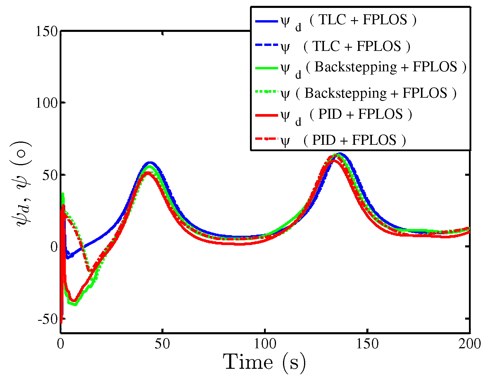
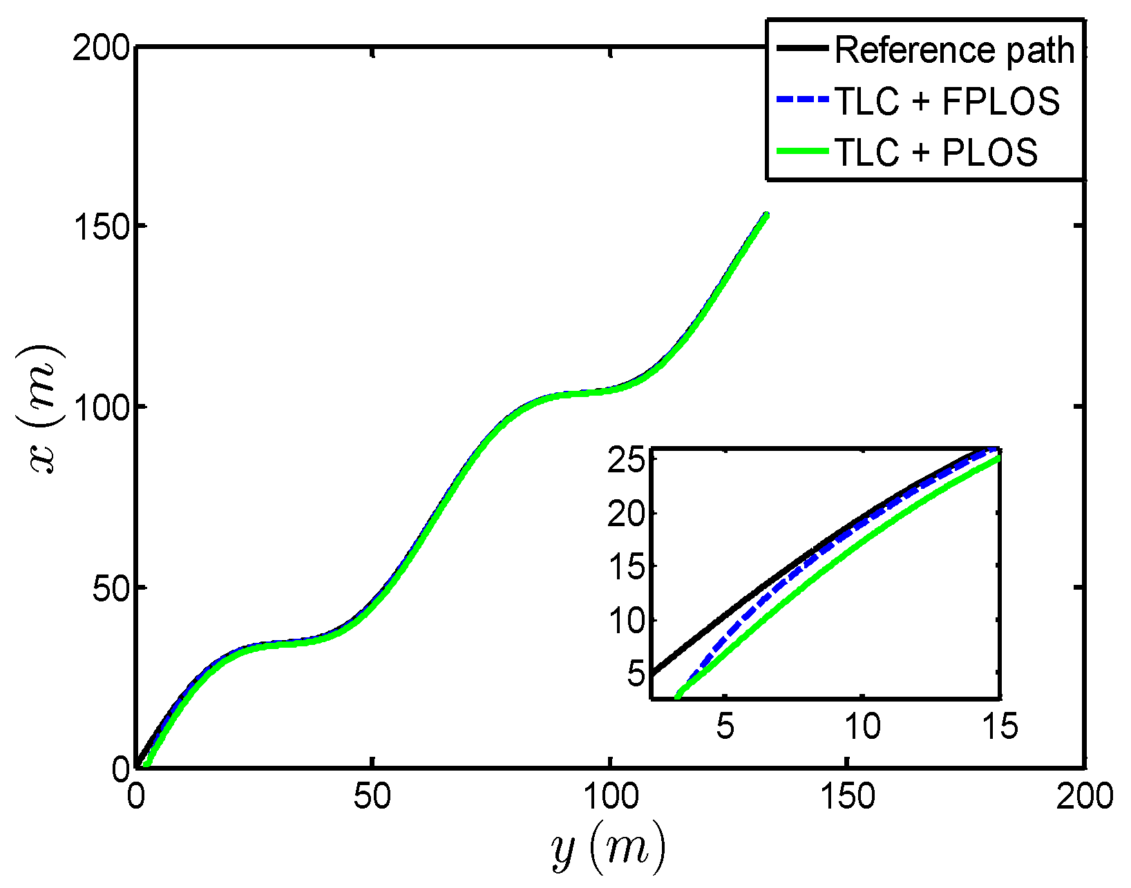
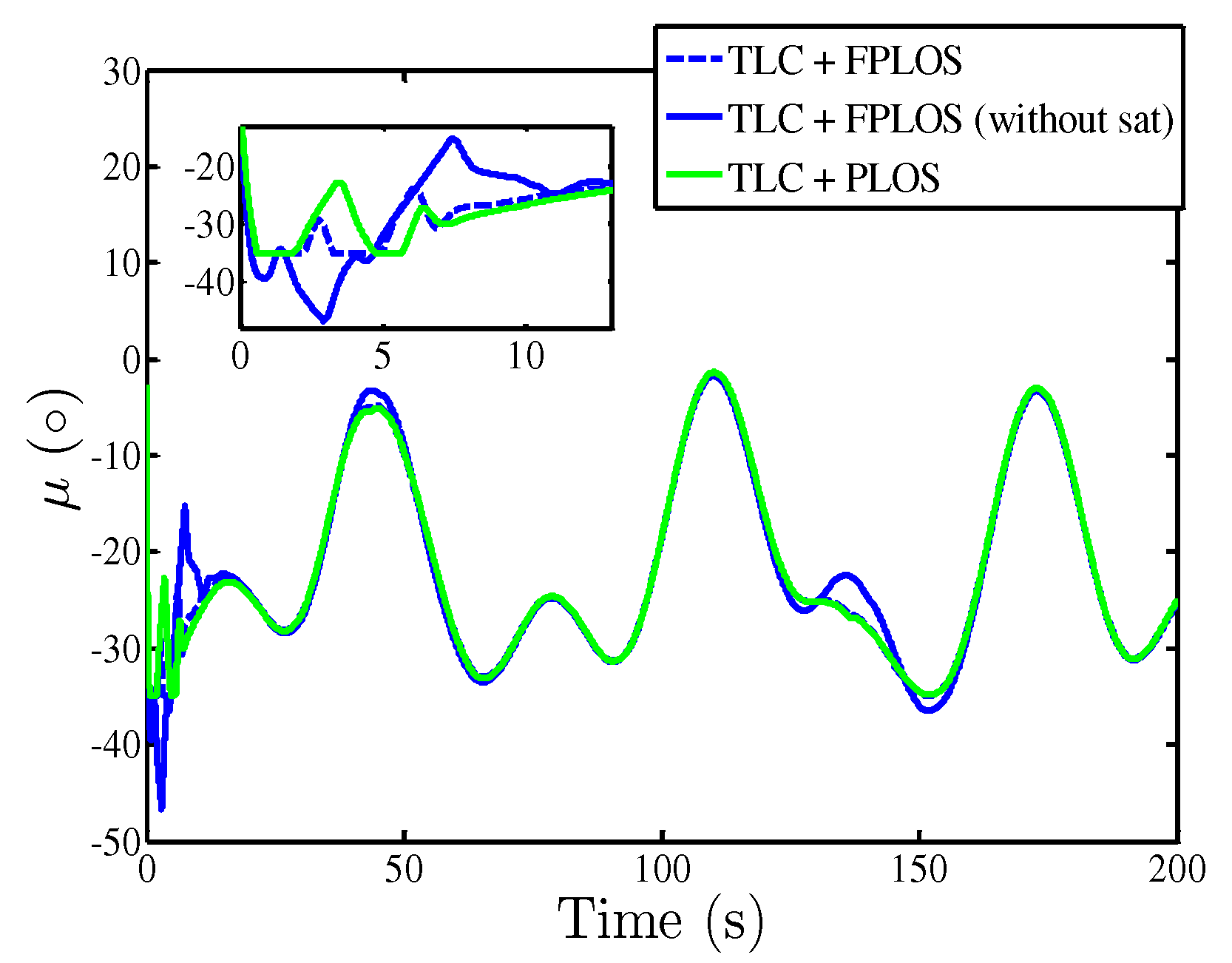
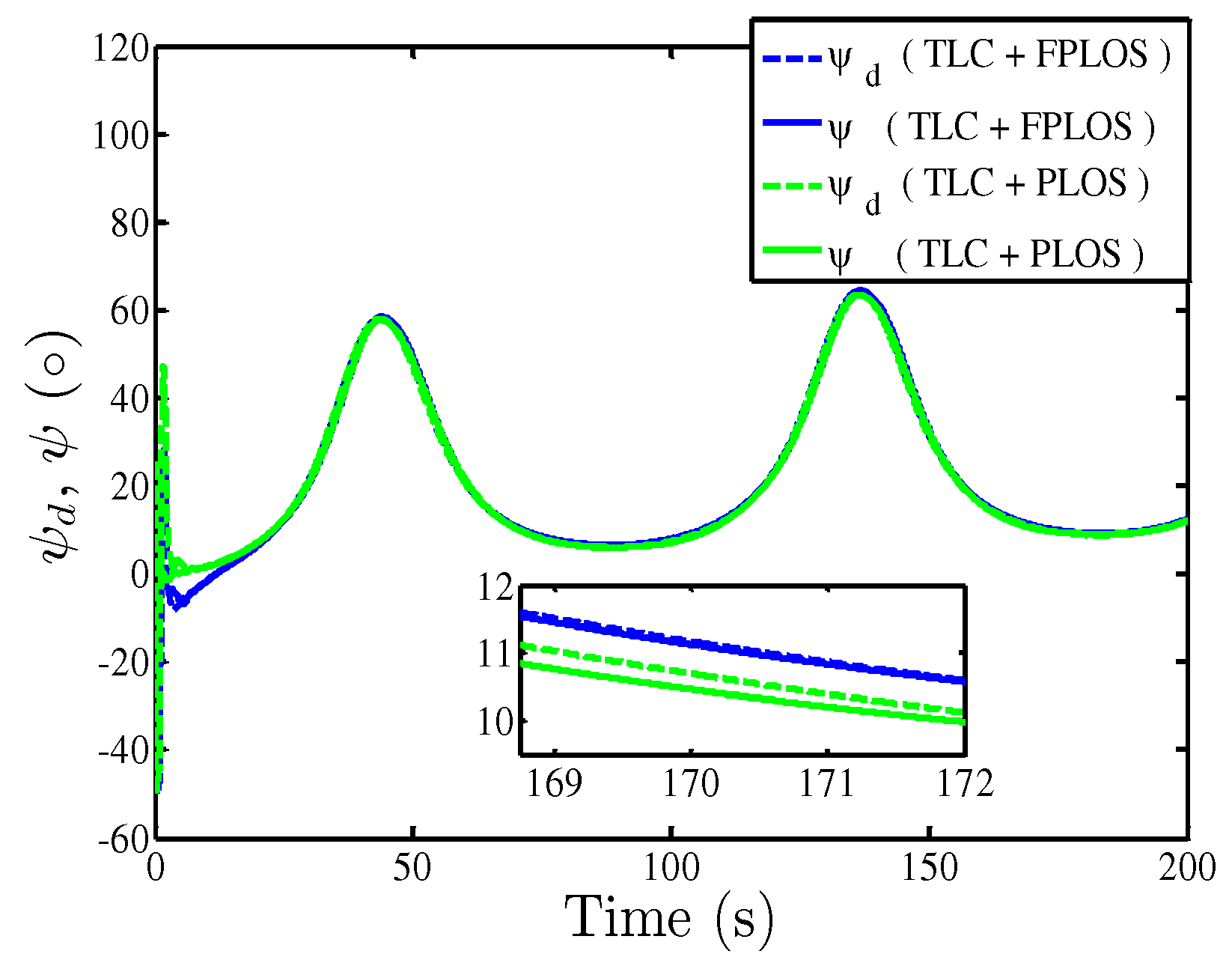
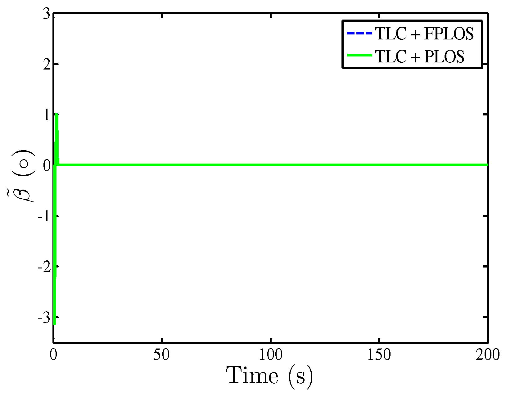
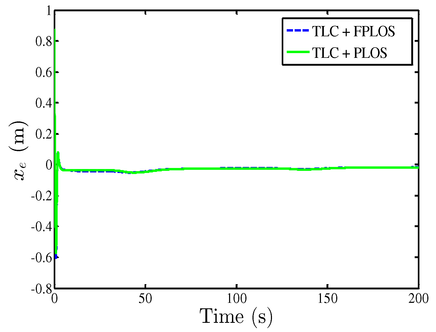
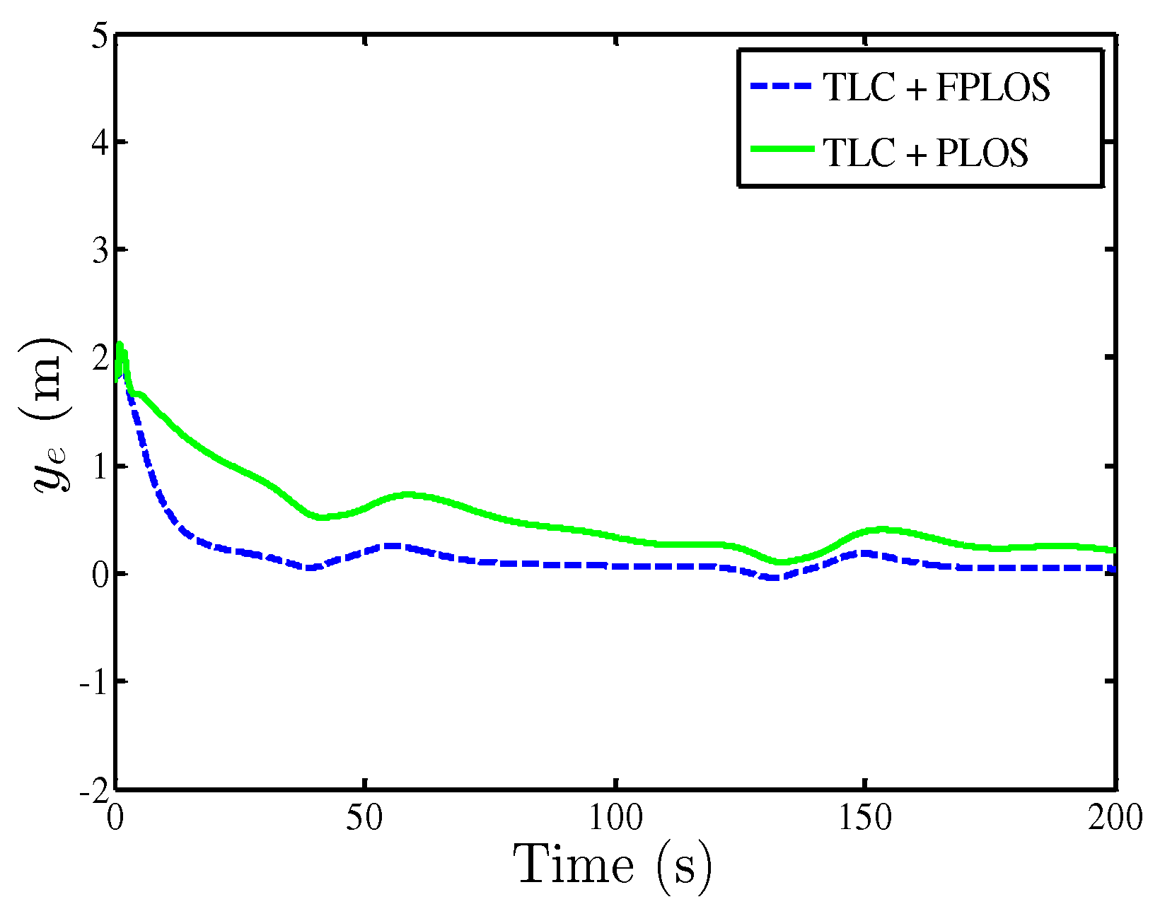
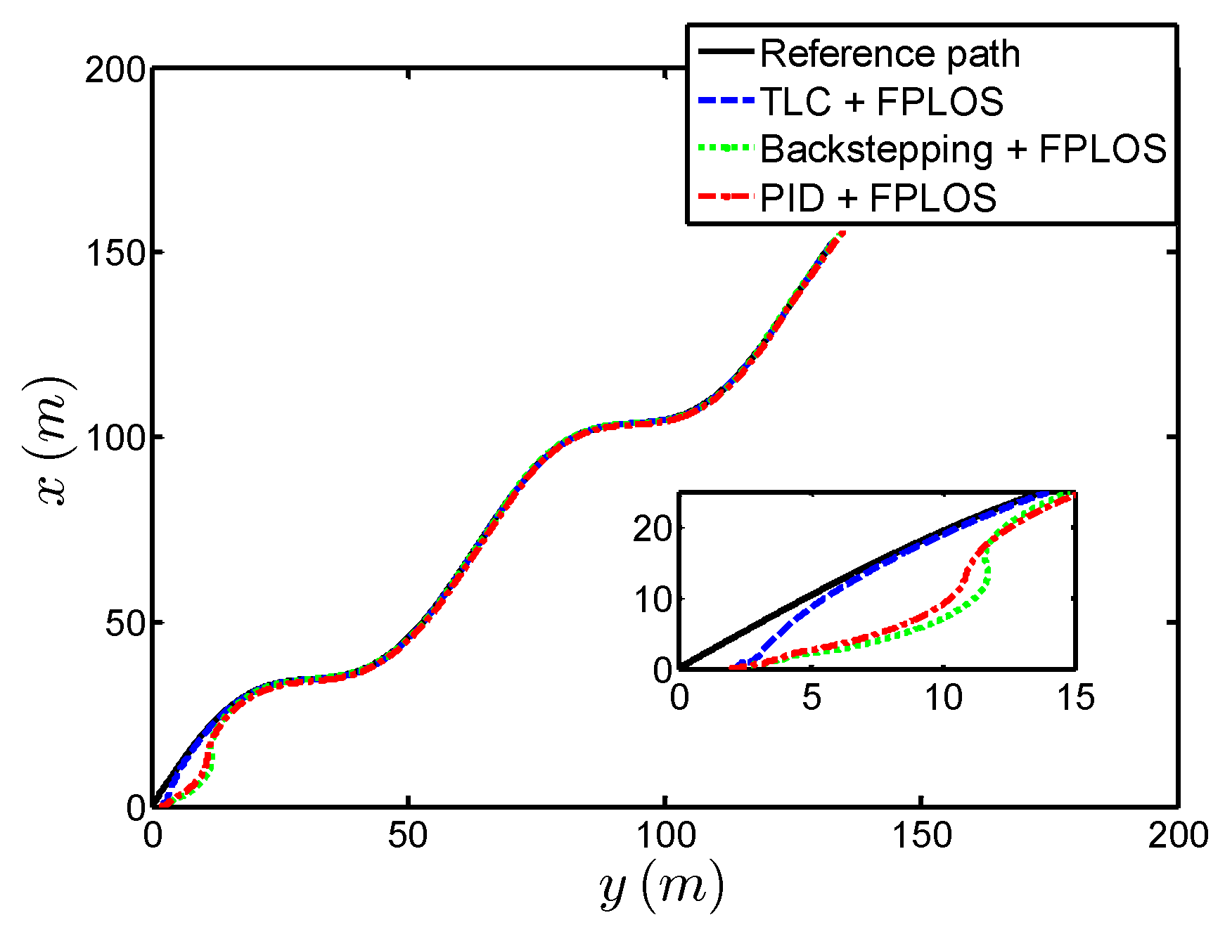
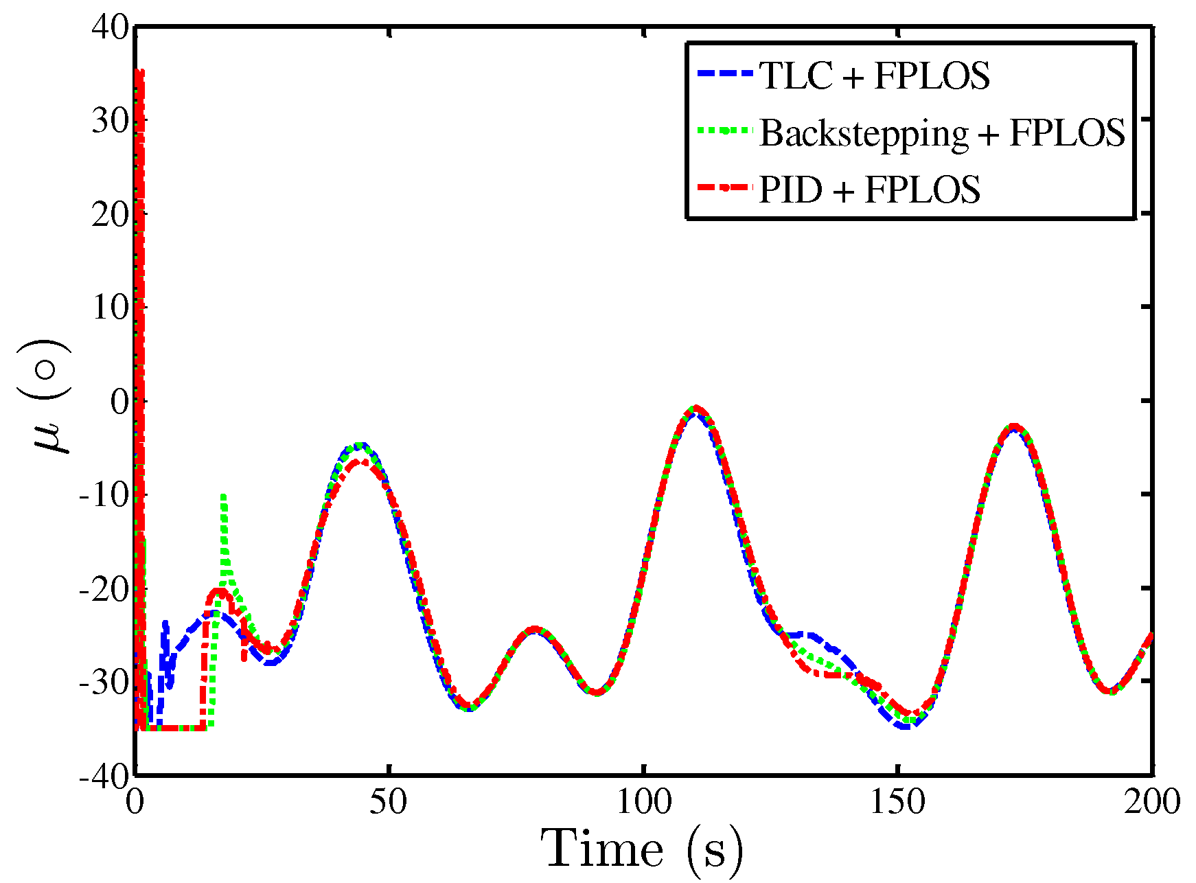
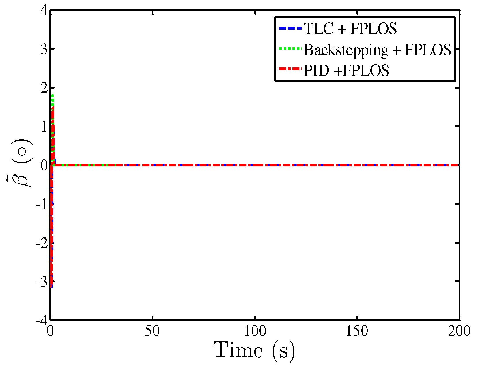
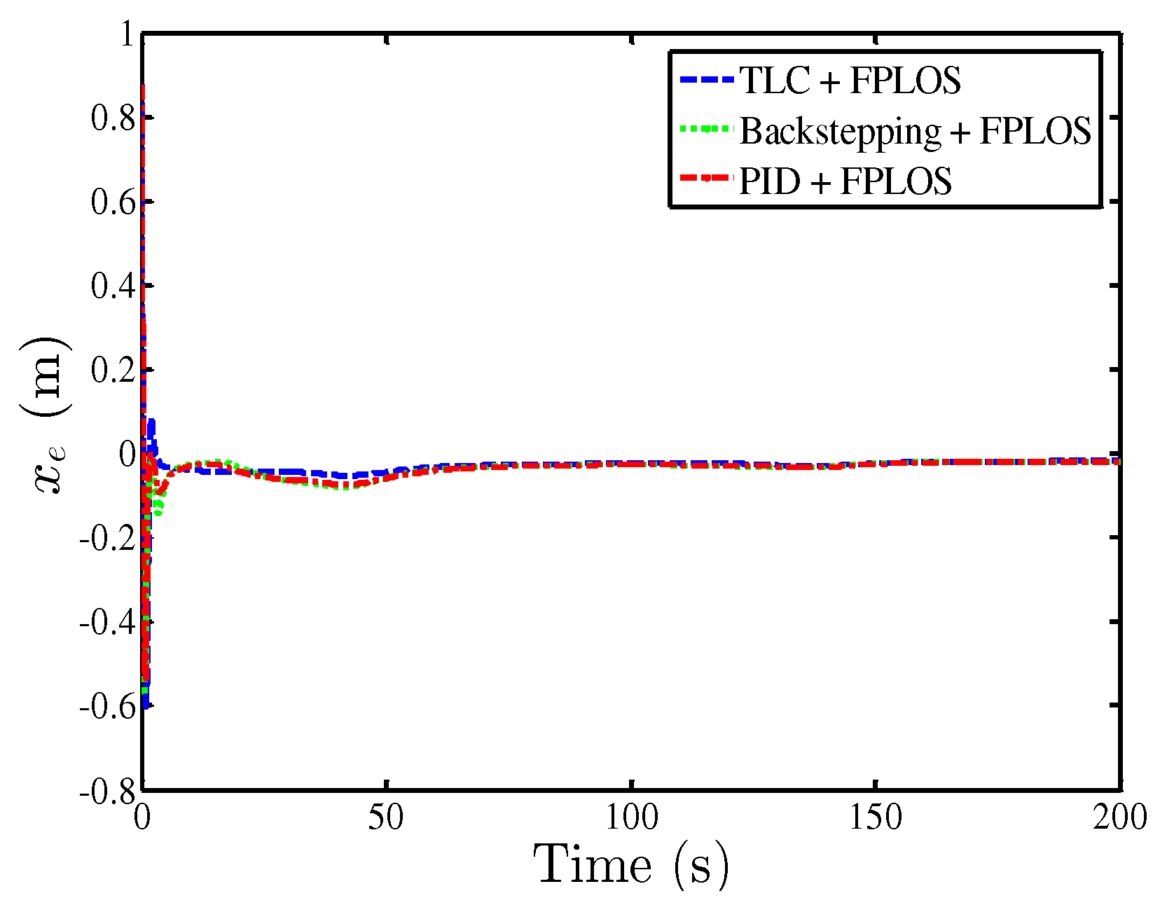
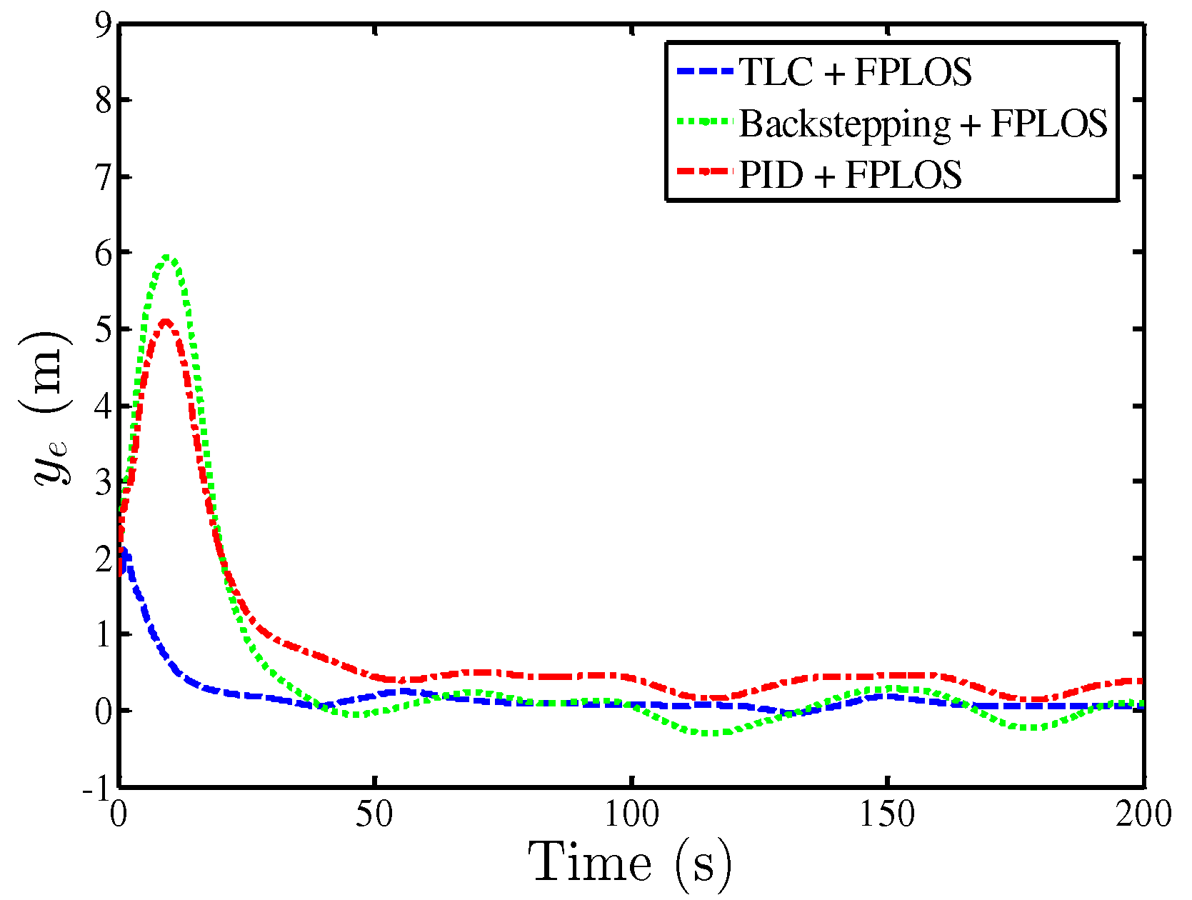
5. Numerical Simulations

In this section, we conduct simulation studies using the MATLAB/Simulink environment. Meanwhile, two cases are applied to evaluate the performance of the proposed strategy, and the simulation results are compared with PLOS [13], the backstepping adaptive method [39], and the PID method. In addition, the following root mean squared error (RMSE) and mean integral absolute (MIA) value describing the error ${\pi }_e\left(\tau \right)$ are considered:

$$\begin{array}{c}\hfill \begin{array}{c}RMSE={\sum }_{i=1}^N\sqrt{\frac{{\left|{\pi }_e\left(\tau \right)\right|}^2}{N}}\hfill \\ MIA=\frac{1}{t_{\infty }-t_0}{\int }_{t_0}^{t_{\infty }}\left|{\pi }_e\left(\tau \right)\right|d\tau \hfill \end{array}\end{array}$$

(57)

where N is the number of simulation steps.

The parameters of the USV can be obtained by [29], and the initial value is ${\left[x,y,\psi \right]}^T={\left[0,2,0\right]}^T$, ${\left[u,v,r\right]}^T={\left[1,0,0\right]}^T$. The design parameters are chosen as follows: $Q\left(t\right)=0.5I_{4\times 4}$, $k_x=3$, $k_y=2$, $k_1=8$, $\gamma =5$, ${\Delta }_{max}=6$, ${\Delta }_{min}=2$, $R_1=0.06$, $h_1=0.02$, ${\sigma }_1=10$, ${\kappa }_1=2$, ${\sigma }_2=0.001$, ${\kappa }_2=0.02$, ${\omega }_j=1.5\left(j=1,2\right)$, ${\varpi }_1=10$, $K_{\mathsf{\Theta }}=2$, ${\chi }_1=0.1$, $K_n=3$. The desired path is chosen as ${\left[x_d,y_d\right]}^T={\left[10sin\left(0.1\theta \right)+1.1\theta ,\theta \right]}^T$. In addition, the unmodeled dynamics and the time-varying external disturbances are selected as $\Delta f=0.3f\left(r\right)$, $d\left(t\right)=0.8+0.4sin\left(0.1t\right)+0.3cos\left(0.2t\right)$, respectively.

Remark 4.

It is worth noting that we can improve the control ability of the controller by choosing appropriate design parameters. For example: the bandwidth ${\omega }_j$ of enhanced TLC is selected by the pole assignment technique; $R_1$ of NTD is relatively sensitive. As $R_1$ becomes larger, the tracking speed becomes faster; as ${\varpi }_1$ of LESO increases, the error $\tilde{d}$ will become smaller. Therefore, we should choose the parameters according to the actual situation.

Case 1. To verify the performance of the FPLOS guidance law, a comparison simulation is conducted between FPLOS and PLOS under the same design parameters.

Simulation results are provided in Figure 5, Figure 6, Figure 7, Figure 8, Figure 9 and Figure 10, and the performance indices are reported in

Table 1. Performance comparisons of different methods. MIA, mean integral absolute. FPLOS, fuzzy predictor line-of-sight.

	Value
Method	$\mathit{RMSE}\left({\mathit{x}}_{\mathit{e}}\right)$	$\mathit{RMSE}\left({\mathit{y}}_{\mathit{e}}\right)$	$\mathit{RMSE}\left({\mathit{E}}_1\right)$	$\mathit{MIA}\left({\mathit{x}}_{\mathit{e}}\right)$	$\mathit{MIA}\left({\mathit{y}}_{\mathit{e}}\right)$	$\mathit{MIA}\left({\mathit{E}}_1\right)$
TLC + FPLOS	0.04941	0.3473	0.06539	0.03204	0.176	0.0139
TLC + PLOS	0.5242	0.6508	0.07489	0.04284	0.523	0.04631

. Figure 5 shows that the designed FPLOS provides faster convergence speed and tracking performance than PLOS. The control inputs are given in Figure 6, and it is noted that the rudder saturation problem was effectively compensated by the auxiliary system. Figure 7 depicts that the actual heading could accurately track the desired heading using the designed FPLOS. Figure 8 depicts that the predictor was capable of identifying unknown sideslip angle. The errors $x_e$ and $y_e$ are shown in Figure 9 and Figure 10. It can be seen from Figure 10 that $y_e$ had fast convergence performance using the proposed FPLOS. The main reason was that the lookahead distance $\Delta$ was optimized reasonably by the fuzzy algorithm, thus achieving better convergence quality. It is shown from Table 1 that the RMSE and MIA values of FPLOS were $\left[0.04941,0.3473,0.06539\right]$, $\left[0.03204,0.176,0.0139\right]$, respectively, and they were only $\left[9.42\%,53.3\%,87\%\right]$ and $\left[74.7\%,33.65\%,30.01\%\right]$ of PLOS. Therefore, the designed FPLOS had better performance in terms of the convergence and stability.

Case 2. Under the same condition and design parameters as Case 1, to prove the effectiveness of the designed TLC method, we provide a comparative simulation in TLC, backstepping, and the PID method.

Simulation results are displayed in Figure 11, Figure 12, Figure 13, Figure 14, Figure 15 and Figure 16, and the performance indices are summarized in

Table 2. Performance comparisons of different methods.

	Value
Method	$\mathit{RMSE}\left({\mathit{x}}_{\mathit{e}}\right)$	$\mathit{RMSE}\left({\mathit{y}}_{\mathit{e}}\right)$	$\mathit{RMSE}\left({\mathit{E}}_1\right)$	$\mathit{MIA}\left({\mathit{x}}_{\mathit{e}}\right)$	$\mathit{MIA}\left({\mathit{y}}_{\mathit{e}}\right)$	$\mathit{MIA}\left({\mathit{E}}_1\right)$
TLC + FPLOS	0.04941	0.3473	0.06539	0.03204	0.176	0.0139
Backstepping + FPLOS	0.05564	1.501	0.2142	0.03753	0.6259	0.08243
PID + FPLOS	0.0549	1.354	0.191	0.0376	0.797	0.0864

. Figure 11 presents the comparisons of the control performance, from which we can find that the designed TLC method exhibited better convergence performance than backstepping and the PID method even though being perturbed by unknown dynamics and external disturbances. Figure 12 depicts that the calculated control input exceeded the operation condition of the actuators, thus causing the problem of rudder saturation. It can also be seen from Figure 12 that an auxiliary system was incorporated into the proposed controller to handle this problem. Figure 13 shows that the actual heading could track the guidance heading with arbitrarily small error. Figure 14 demonstrates sideslip angle estimation errors, and it can be clearly observed that the predictor could accurately estimate unknown sideslip angle. Figure 15 and Figure 16 illustrate the tracking errors of the three control methods. It was evident that the errors of the designed TLC method could quickly converge to a small region around the origin. However, the errors of backstepping and PID were still fluctuating. Table 2 summarizes the comparison of the RMSE and MIA values of the three methods. It can be easily seen that the designed TLC method had higher tracking precision. All results demonstrated that our proposed control strategy exhibited superior control performance.

6. Conclusions

In this paper, a novel path following control strategy was proposed for a USV subject to unmodeled dynamics, external disturbance, and rudder saturation. First, an FPLOS guidance strategy was developed to provide the guidance heading, which could also handle unknown sideslip angle. More importantly, the greatest advantage was that TLC was used as a new effective technique to design a concise path following controller, and the proposed controller could not only estimate and compensate for unknown dynamics and rudder saturation, but also provide high tracking precision. Meanwhile, NTD was applied in the proposed strategy to avoid unnecessary set-point jump. The superiority and the effectiveness of the proposed strategy were also confirmed by comparisons and extensive simulations. In the future, we will further optimize the lookahead distance using other methods [40,41,42,43,44], and the proposed design methods could also be used to solve the trajectory tracking problem of the USV and underwater vehicle.

References

1. Liu, Y.C.; Bucknall, R. Efficient multi-task allocation and path planning for unmanned surface vehicle in support of ocean operations. Neurocomputing 2018, 275, 142–149. [Google Scholar] [CrossRef]
2. Song, R.; Liu, Y.; Bucknall, R. A multi-layered fast marching method for unmanned surface vehicle path planning in a time-variant maritime environment. Ocean Eng. 2018, 129, 301–317. [Google Scholar] [CrossRef]
3. Zhao, Y.X.; Li, W.; Shi, P. A real-time collision avoidance learning system for Unmanned Surface Vessels. Neurocomputing 2016, 182, 255–266. [Google Scholar] [CrossRef]
4. Liu, L.; Wang, D.; Peng, Z.H. Path following of marine surface vehicles with dynamical uncertainty and time-varying ocean disturbances. Neurocomputing 2016, 173, 799–808. [Google Scholar] [CrossRef]
5. Oh, S.R.; Sun, J. Path following of underactuated marine surface vessels using line-of-sight based model predictive control. Ocean Eng. 2010, 3, 289–295. [Google Scholar] [CrossRef]
6. Peymani, E.; Fossen, T.I. Path following of underwater robots using Lagrange multipliers. Robot. Auton. Syst. 2015, 67, 44–52. [Google Scholar] [CrossRef]
7. Zheng, Z.W.; Sun, L. Path following control for marine surface vessel with uncertainties and input saturation. Neurocomputing 2016, 177, 158–167. [Google Scholar] [CrossRef]
8. Zhang, G.Q.; Zhang, X.K.; Zheng, Y.F. Adaptive neural path-following control for underactuated ships in fields of marine practice. Ocean Eng. 2015, 104, 558–567. [Google Scholar] [CrossRef]
9. Paliotta, C.; Lefeber, E.; Pettersen, K.Y.; Pinto, J.; Costa, M. Trajectory Tracking and Path Following for Underactuated Marine Vehicles. IEEE Trans. Control Syst. Technol. 2019, 27, 1423–1437. [Google Scholar] [CrossRef] [Green Version]
10. Fossen, T.I.; Lekkas, A.M. Direct and indirect adaptive integral line-of-sight path-following controllers for marine craft exposed to ocean currents. Int. J. Adapt. Control Signal Process. 2017, 31, 445–463. [Google Scholar] [CrossRef]
11. Zheng, Z.; Sun, L.; Xie, L.H. Error-Constrained LOS Path Following of a Surface Vessel with Actuator Saturation and Faults. IEEE Trans. Syst. Man Cybern. Syst. 2018, 48, 1794–1805. [Google Scholar] [CrossRef]
12. Wang, N.; Sun, Z.; Yin, J.C.; Su, S.F.; Sharma, S. Finite-Time Observer Based Guidance and Control of Underactuated Surface Vehicles with Unknown Sideslip Angles and Disturbances. IEEE Access 2018, 6, 14059–14070. [Google Scholar] [CrossRef]
13. Liu, L.; Wang, D.; Peng, Z.H.; Wang, H. Predictor-based LOS guidance law for path following of underactuated marine surface vehicles with sideslip compensation. Ocean Eng. 2016, 124, 340–348. [Google Scholar] [CrossRef]
14. Lekkas, A.M.; Fossen, T.I. Integral LOS path following for curved paths based on a monotone cubic Hermite spline parametrization. IEEE Trans. Control Syst. Technol. 2014, 22, 2287–2301. [Google Scholar] [CrossRef]
15. Liu, L.; Wang, D.; Peng, Z.H. ESO-Based Line-of-Sight Guidance Law for Path Following of Underactuated Marine Surface Vehicles with Exact Sideslip Compensation. IEEE J. Ocean. Eng. 2017, 42, 477–487. [Google Scholar] [CrossRef]
16. Wang, N.; Sun, Z.; Zheng, Z.; Zhao, H. Finite-Time Sideslip Observer-Based Adaptive Fuzzy Path-Following Control of Underactuated Marine Vehicles with Time-Varying Large Sideslip. Int. J. Fuzzy Syst. 2018, 20, 1767–1778. [Google Scholar] [CrossRef]
17. Fossen, T.I.; Pettersen, K.Y.; Galeazzi, R. Line-of-sight path following for dubins paths with adaptive sideslip compensation of drift forces. IEEE Trans. Control Syst. Technol. 2015, 23, 820–827. [Google Scholar] [CrossRef] [Green Version]
18. Peng, Z.; Wang, J.; Wang, D. Distributed Maneuvering of Autonomous Surface Vehicles Based on Neurodynamic Optimization and Fuzzy Approximation. IEEE Trans. Control Syst. Technol. 2017, 99, 1–8. [Google Scholar] [CrossRef]
19. Wang, N.; Meng, J.E. Direct Adaptive Fuzzy Tracking Control of Marine Vehicles With Fully Unknown Parametric Dynamics and Uncertainties. IEEE Trans. Control Syst. Technol. 2016, 24, 1845–1852. [Google Scholar] [CrossRef]
20. Mu, D.; Wang, G.; Fan, Y.; Sun, X.; Qiu, B. Adaptive LOS Path Following for a Podded Propulsion Unmanned Surface Vehicle with Uncertainty of Model and Actuator Saturation. Appl. Sci. 2017, 7, 1232. [Google Scholar] [CrossRef] [Green Version]
21. Shao, X.; Wang, H. Active disturbance rejection based trajectory linearization control for hypersonic reentry vehicle with bounded uncertainties. ISA Trans. 2015, 54, 27–38. [Google Scholar] [CrossRef] [PubMed]
22. Shao, X.; Wang, H. Back-stepping robust trajectory linearization control for hypersonic reentry vehicle via novel tracking differentiator. J. Frankl. Inst. 2016, 353, 1957–1984. [Google Scholar] [CrossRef]
23. Wang, N.; Er, M.J.; Sun, J.C.; Liu, Y.C. Adaptive Robust Online Constructive Fuzzy Control of a Complex Surface Vehicle System. IEEE Trans. Cybern. 2016, 46, 1511–1523. [Google Scholar] [CrossRef] [PubMed]
24. He, W.; Dong, Y.; Sun, C. Adaptive Neural Impedance Control of a Robotic Manipulator With Input Saturation. IEEE Trans. Syst. Man Cybern. Syst. 2017, 46, 334–344. [Google Scholar] [CrossRef]
25. Yu, Y.; Guo, C.; Yu, H. Finite-time predictor line-of-sight-based adaptive neural network path following for unmanned surface vessels with unknown dynamics and input saturation. Int. J. Adv. Robot. Syst. 2018, 15. [Google Scholar] [CrossRef]
26. Zheng, Z.; Feroskhan, M. Path Following of a Surface Vessel With Prescribed Performance in the Presence of Input Saturation and External Disturbances. ASME Trans. Mechatron. 2017, 22, 2564–2575. [Google Scholar] [CrossRef]
27. Du, J.; Hu, X.; Sun, Y. Adaptive Robust Nonlinear Control Design for Course Tracking of Ships Subject to External Disturbances and Input Saturation. IEEE Trans. Syst. Man Cybern. Syst. 2020, 50, 193–202. [Google Scholar] [CrossRef]
28. Zhu, G.; Du, J. Global Robust Adaptive Trajectory Tracking Control for Surface Ships Under Input Saturation. IEEE J. Ocean. Eng. 2018, 45, 442–450. [Google Scholar] [CrossRef]
29. Mu, D.; Wang, F.; Fan, Y.; Qiu, B.; Sun, X. Adaptive course control based on trajectory linearization control for unmanned surface vehicle with unmodeled dynamics and input saturation. Neurocomputing 2019, 330, 1–10. [Google Scholar] [CrossRef]
30. Breivik, M.; Hovstein, V.E.; Fossen, T.I. Straight-line target tracking for unmanned surface vehicles. Model. Identif. Control 2008, 29, 131–149. [Google Scholar] [CrossRef] [Green Version]
31. Khalil, H.K. Nonlinear Systems; Prentice Hall: New York, NY, USA, 1996. [Google Scholar]
32. Mickle, M.C.; Zhu, J.J. Skid to turn control of the APKWS missile using trajectory linearization technique. In Proceedings of the 2001 American Control Conference, Arlington, VA, USA, 25–27 June 2001; Volume 5, pp. 3346–3351. [Google Scholar]
33. Zhu, B.; Huo, W. Adaptive Trajectory Linearization Control for a model-scaled helicopter with uncertain inertial parameters. In Proceedings of the 31st Chinese Control Conference, Hefei, China, 25–27 July 2012; Volume 5, pp. 4389–4395. [Google Scholar]
34. Adami, T.M.; Zhu, J. 6DOF flight control of fixed-wing aircraft by Trajectory Linearization. In Proceedings of the 2011 American Control Conference, San Francisco, CA, USA, 29 June–1 July 2011; pp. 1610–1617. [Google Scholar]
35. Chen, Y.; Zhu, J. Car-like ground vehicle trajectory tracking by using trajectory linearization control. In Proceedings of the ASME 2017 Dynamic Systems and Control Conference, Tysons, VA, USA, 11–13 October 2017; Volume 2. [Google Scholar]
36. Huang, J.T. Global tracking control of strict-feedback systems using neural networks. IEEE Trans. Neural Netw. Learn. Syst. 2012, 23, 1714–1725. [Google Scholar] [CrossRef] [PubMed]
37. Han, J. From PID to active disturbance rejection control. IEEE Trans. Ind. Electron. 2009, 56, 900–906. [Google Scholar] [CrossRef]
38. Qiu, B.; Wang, G.; Fan, Y. Robust Adaptive Trajectory Linearization Control for Tracking Control of Surface Vessels with Modeling Uncertainties under Input Saturation. IEEE Access 2019, 7, 5057–5070. [Google Scholar] [CrossRef]
39. Lin, Y.; Du, J.; Niu, J. Design of Backstepping based adaptive robust nonlinear controller of ship course. Ship Eng. 2007, 29, 24–27. [Google Scholar]
40. Guerra, E.H.; Quiza, R.; Villalonga, A.; Arenas, J.; Castano, F. Digital Twin-Based Optimization for Ultraprecision Motion Systems with Backlash and Friction. IEEE Access 2019, 7, 93462–93472. [Google Scholar] [CrossRef]
41. Beruvides, G.; Juanes, C.; Castano, F.; Haber, R.E. A self-learning strategy for artificial cognitive control systems. In Proceedings of the 2015 IEEE 13th International Conference on Industrial Informatics (INDIN), Cambridge, UK, 22–24 July 2015; pp. 1180–1185. [Google Scholar]
42. Martin, A.G.; Guerra, E.H. Internal model control based on a neurofuzzy system for network applications. A case study on the high-performance drilling process. IEEE Trans. Autom. Sci. Eng. 2009, 6, 367–372. [Google Scholar] [CrossRef]
43. Guerra, E.H.; Alique, A.; Alique, J.R. Tool wear prediction in milling using neural networks. Lect. Notes Comput. Sci. 2002, 2415, 807–812. [Google Scholar]
44. Ebrahimi, Z.; Shahabi, H.; Soltani, M. Reinforcement learning for optimal scheduling of Glioblastoma treatment with Temozolomide. Comput. Methods Programs Biomed. 2020, 193, 105443. [Google Scholar] [CrossRef]
Figure 1. The Earth-fixed inertial and the body-fixed frame.
Applsci 10 03538 g001
Figure 2. TLC scheme diagram.
Applsci 10 03538 g002
Figure 3. The block diagram of the proposed control strategy for the USV.
Applsci 10 03538 g003
Figure 4. Geometrical illustration of LOS guidance.
Applsci 10 03538 g004
Figure 5. Path following performance.
Applsci 10 03538 g005
Figure 6. Control inputs μ .
Applsci 10 03538 g006
Figure 7. Guidance heading ψ d and heading ψ .
Applsci 10 03538 g007
Figure 8. Sideslip angle estimation errors β ˜ .
Applsci 10 03538 g008
Figure 9. Along-track errors x e .
Applsci 10 03538 g009
Figure 10. Cross-track errors y e .
Applsci 10 03538 g010
Figure 11. Path following performance.
Applsci 10 03538 g011
Figure 12. Control inputs μ .
Applsci 10 03538 g012
Figure 13. Guidance heading ψ d and heading ψ .
Applsci 10 03538 g013
Figure 14. Sideslip angle estimation errors β ˜ .
Applsci 10 03538 g014
Figure 15. Along-track errors x e .
Applsci 10 03538 g015
Figure 16. Cross-track errors y e .
Applsci 10 03538 g016