A Data-Independent Genetic Algorithm Framework for Fault-Type Classification and Remaining Useful Life Prediction

Featured Application

We propose a data-independent framework based on an ensemble of genetic algorithms for fault-type classification and remaining useful life prediction.

Abstract

Machinery diagnostics and prognostics usually involve the prediction process of fault-types and remaining useful life (RUL) of a machine, respectively. The process of developing a data-driven diagnostics and prognostics method involves some fundamental subtasks such as data rebalancing, feature extraction, dimension reduction, and machine learning. In general, the best performing algorithm and the optimal hyper-parameters suitable for each subtask are varied across the characteristics of datasets. Therefore, it is challenging to develop a general diagnostic/prognostic framework that can automatically identify the best subtask algorithms and the optimal involved parameters for a given dataset. To resolve this problem, we propose a new framework based on an ensemble of genetic algorithms (GAs) that can be used for both the fault-type classification and RUL prediction. Our GA is combined with a specific machine-learning method and then tries to select the best algorithm and optimize the involved parameter values in each subtask. In addition, our method constructs an ensemble of various prediction models found by the GAs. Our method was compared to a traditional grid-search over three benchmark datasets of the fault-type classification and the RUL prediction problems and showed a significantly better performance than the latter. Taken together, our framework can be an effective approach for the fault-type and RUL prediction of various machinery systems.

1. Introduction

In a machinery system, diagnostics and prognostics usually involve two kinds of problems, a fault-type classification and a remaining useful life (RUL) prediction problem. In particular, prognostics has been applied to the field of machinery maintenance as it allows industries to better plan logistics, as well as save cost by conducting maintenance only when needed [1]. Various approaches have been proposed in each problem and they can be divided into three categories: Physics-based, data-driven, and hybrid-based approaches. Physics-based approaches incorporate prior system-specific knowledge from an expert, as shown in previous studies, of fault-type classification [2,3,4,5] and RUL prediction [6,7,8,9] problems. Alternatively, data-driven approaches are based on statistical-/machine-learning techniques using the historical data (see example studies about fault-type classification [10,11,12,13,14] and RUL estimation [15,16,17,18]). Hybrid-based approaches attempt to utilize the strengths of both approaches, if applicable, by combining knowledge related to the physical process and information obtained from the observed data (see example studies about fault-type classification [19,20,21,22] and RUL prediction [23,24,25,26]). However, physics-based and hybrid-based approaches are limited in practice because the underlying physical models are not available in most real systems. Therefore, data-driven approaches have become increasingly popular along with recent advancements in sensor systems and data storage/analysis techniques.

From a review of the data-driven approaches, we noticed that many different types of learning methods and data pre-processing algorithms have been employed. For example, the fisher discriminative analysis and the support vector machine were used for feature extraction and classification, respectively, to diagnose seven failure modes of three different polymer electrolyte membrane fuel cell systems in a previous study [10]. Another study applied a single hidden-layer feedforward neural network combined with an extreme learning machine technology to identify the offset, stuck, and noise faults in induction motor drive systems [11]. A multi-classification model based on the recurrent neural network was established to classify ten different fault-types of a wind power generation system [27]. A deep convolutional neural network and a random forest ensemble were employed to diagnose faults of a reliance electric motor and a rolling mill [28]. In [29], a genetic algorithm-based optimal feature subset selection and a K-nearest-neighbor classifier were applied to distinguish between normal and crack conditions of a spherical tank. Various approaches have also been tried for the RUL prediction. A previous study presented a new deep feature learning method for the RUL estimation of a bearing through a multiscale convolutional neural network [18]. A support vector machine was applied to predict the RUL of a Li-ion battery [30] and a microwave component [31]. Another study investigated the applicability of the Kalman filter to fuse the estimates of the RUL from five learning methods such as generalized linear models, neural networks, K-nearest neighbors, random forests, and support vector machines, using the field data of an aircraft bleed valve [15].

This literature review indicated that the process of developing data-driven diagnostics and prognostics methods involved some fundamental subtasks such as data rebalancing, feature extraction, dimension reduction, and machine-learning in the fault-type and/or RUL prediction problems. In addition, the best performing algorithm in each subtask was varied across the characteristics of the given dataset. Moreover, each algorithm required appropriate specification of a number of hyper-parameters. Therefore, it is always challenging to develop a general diagnostics/prognostics framework that can automatically identify the best subtask algorithms and optimize the involved parameters for a given dataset. Although such a general framework does not produce the prediction function that can be common to different systems, it can save the costs in developing diagnostic or prognostic functions by re-executing it. 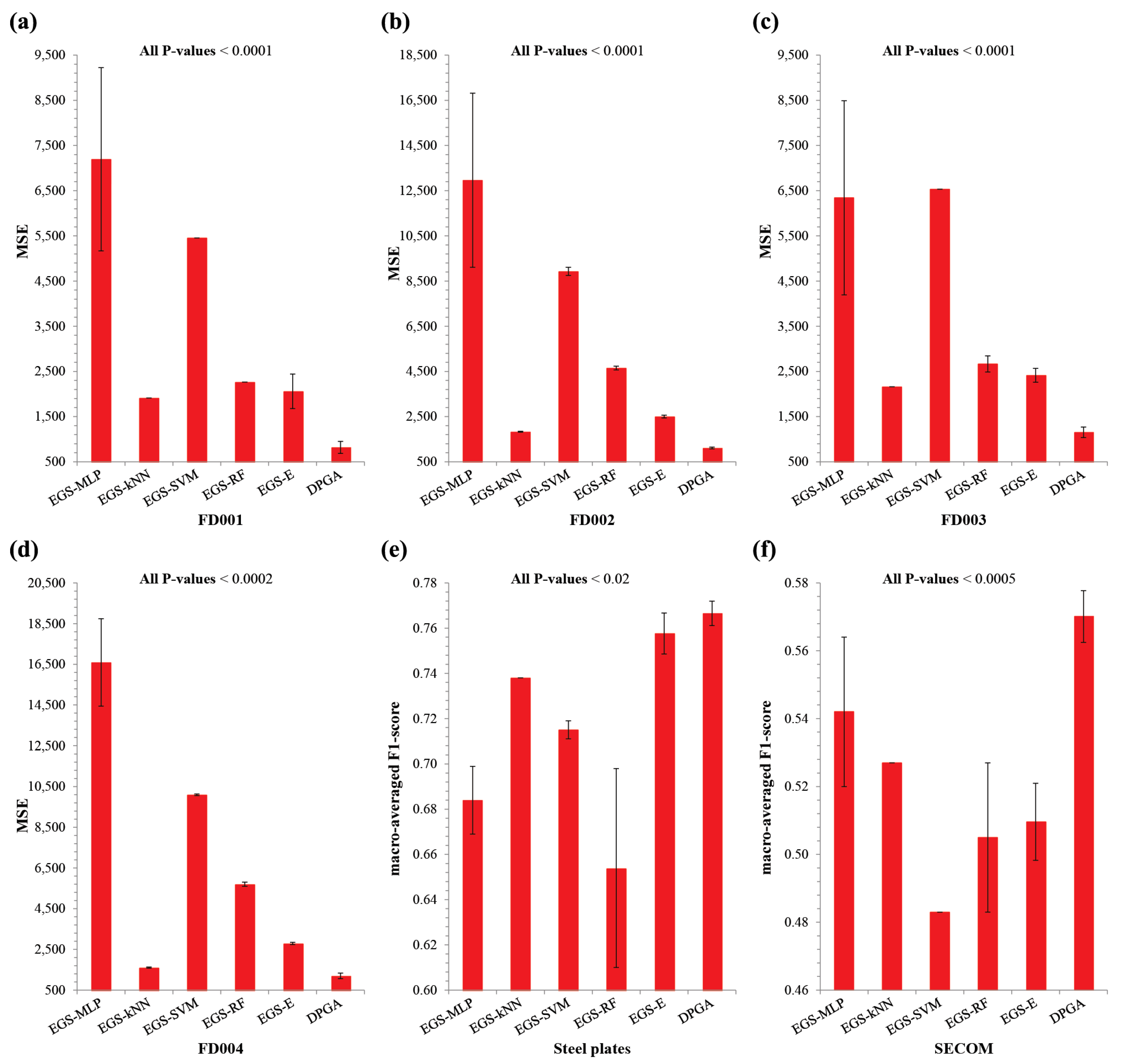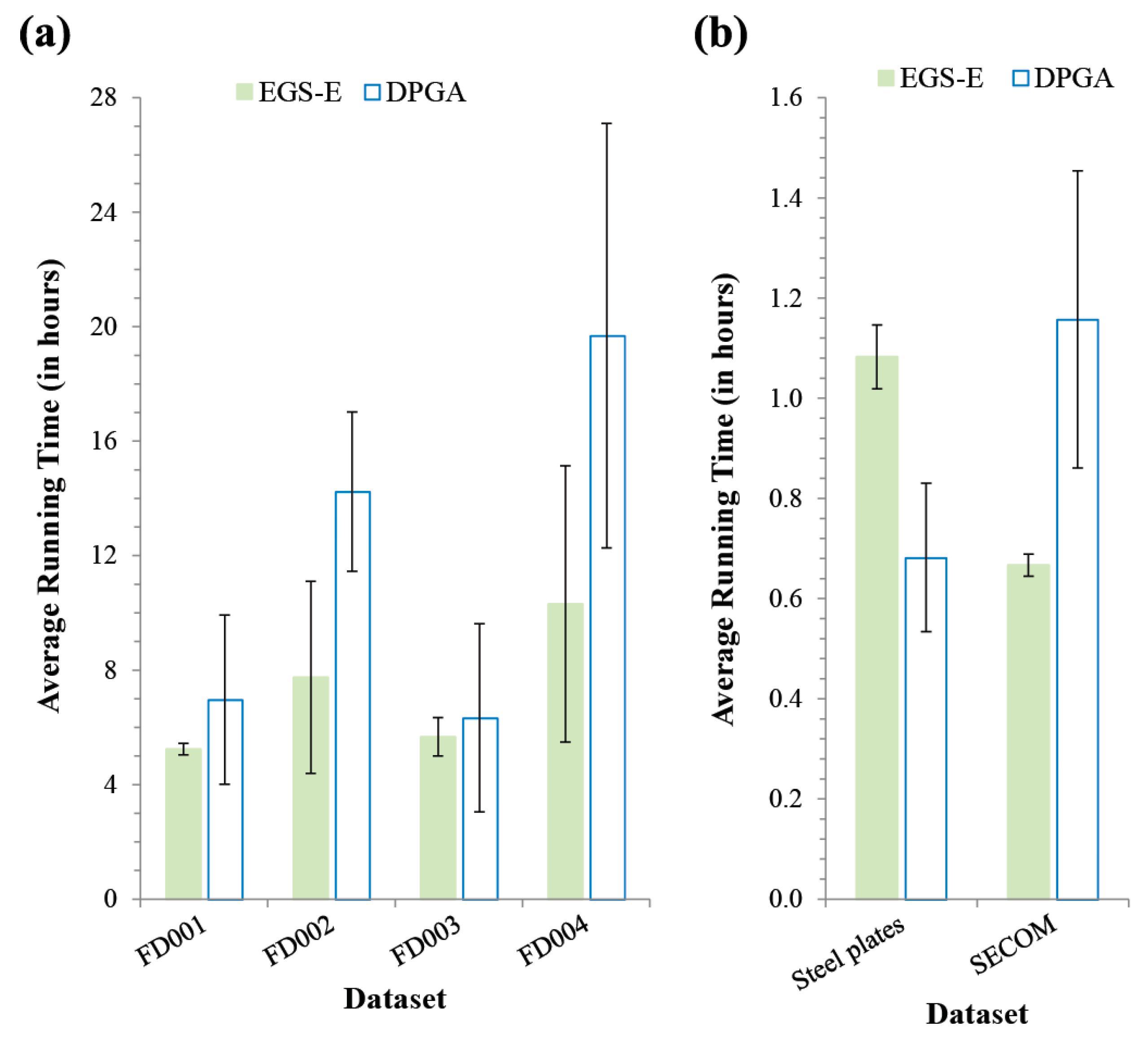The most straightforward approaches for this purpose are the exhaustive grid search [32], which examines a subset of parameters with a constant interval, and the experience-based manual selection [33], where a human expert specifies the parameter values based on their experience. However, the former can be inefficient due to the expensive computational cost, and the latter is dependent on the expert’s knowledge, which is not general to various datasets. In this regard, there is a pressing need to develop an efficient and data-independent approach, so we propose a new framework to develop a diagnostics and prognostics method based on an ensemble of genetic algorithms (GAs) that can be applied for both the fault-type classification and RUL prediction problems. Our framework handles four subtasks such as the data rebalancing, feature extraction, feature reduction, and machine-learning. Accordingly, our GA tries to select the optimal algorithm for each subtask and specify the optimal parameter values involved in the selected algorithm. In addition, the proposed method constructs an ensemble of the prediction models that are found by the GAs combined with various machine-learning methods. To verify the usefulness of our approach, we compared it to a traditional grid-search over three benchmark datasets of the fault-type classification (the steel plates faults and SECOM datasets) and the RUL prediction (NASA commercial modular aero-propulsion system simulation (C-MAPSS) dataset) problems. Our method showed a significantly better and more robust performance than the latter, with a practically acceptable running time.

The remainder of this paper is organized as follows. Section 2 introduces the backgrounds on the diagnostics and prognostics problem and the performance evaluation metrics. Section 3 explains the details of our approach and Section 4 presents the experimental results along with discussion. Section 5 includes the concluding remarks and suggestions for future work.

2. Backgrounds

In the fault-type classification and RUL prediction problems, data-preprocessing has a great impact on the performance of machine-learning methods and it is usually implemented by the rebalancing (in a classification problem), filtering, and dimension-reduction methods. They are introduced in the following subsections, and the last subsection explains the performance evaluation metric used in the study.

2.1. Data Rebalancing Methods

In the practical fault-type classification problem, the proportion of samples of the minority class is often severely lower than that of the majority class, which restricts the learning performance. To resolve this problem, the data rebalancing methods are commonly used. They can be classified into the over-sampling method, which adds samples of the minority class, and the under-sampling method, which reduces samples of the majority class. In general, the resampling process is repeated until the balancing ratio, which is defined by the ratio of the number of samples in the minority class over that in the majority class, is equal to or greater than a threshold parameter value $r$ $(0 < r\le 1)$. In the following, we introduce some representative rebalancing methods that were included in our framework.

2.1.1. Over-Sampling Methods

• Random duplication (RDUP)—A sample of the minority class is randomly selected and then duplicated.
• Synthetic minority over sampling technique (SMOTE) [34]—A sample of the minority class is randomly selected and the weighted mean of the nearest neighbors of it is used to produce a new sample of the minority class.
• Borderline-SMOTE [35]—Two SMOTE variant methods, borderline-SMOTE1 (BSMOTE1) and borderline-SMOTE2 (BSMOTE2), were further developed. They are the same as SMOTE except that a new sample of the minority class is produced near the borderline between classes. In addition, BSMOTE1 chooses the nearest neighbor from only the minority class, whereas BSMOTE2 does so from any class.
• Support vector machine (SVM)-SMOTE (SSMOTE) [36,37]—Similar to borderline-SMOTE methods, the new minority-class sample is produced near the borderline but the borderline is determined by the support vector machine classifiers.

2.1.2. Under-Sampling Methods

Under-sampling methods eliminate the samples of the majority class. This might cause the loss of information of the data, which led the under-sampling method to be less popular than the over-sampling of Batista et al. [38].

• Random removal (RREM)—A sample of the majority class is randomly selected for removal.
• Neighborhood cleaning rule (NCL) [39]—A sample of the majority class is selected by Wilson’s edited nearest neighbor rule [40] or a simple 3-nearest-neighbors search [36] for removal.

2.2. Filtering Methods

A filtering method is employed to remove noise from an original signal, and we herein introduce five well-known filtering methods. Let $f_t$ be the value of the feature $f$ at time $t$ in the following.

• Simple moving average (SMA)—SMA is the unweighted average of values over the past time points as follows.

  $$SMA\left(f_t\right)=\frac{f_t+f_{t-1}+\dots +f_{t-n+1}}{n} ,$$

  (1)

  where $n$ is the number of past time-points.
• Central moving average (CMA)—SMA causes a shift in a trend because it considers only the past samples. On the other hand, CMA is the unweighted average of values over both the past and future time points as follows.

  $$CMA\left(f_t\right)=\frac{f_{t-⎣n/2⎦}+\dots +f_{t-1}+f_t+f_{t+1}+\dots +f_{t+⎣n/2⎦}}{n} ,$$

  (2)

  where $n$ is an odd number specifying the number of time points to be averaged.
• Exponential moving average (EMA)—EMA, which is also known as an exponentially weighted moving average (EWMA), is a type of infinite impulse response filter with an exponentially decreasing weighting factor. The EMA of a time-series of the feature $f$ is recursively calculated as follows.

  $$EMA\left(f_t\right)=\{\begin{array}{ll}{f}_t& if t=1\\ \frac{\left(1-\alpha \right)·f_t+\alpha (1-{\alpha }^{t-1})·EMA\left(f_{t-1}\right)}{1-{\alpha }^t}& if t>1\end{array},$$

  (3)

  where, given the total number of observations $N$, $\alpha =e^{-1/N}$ is a constant factor.
• Exponential smoothing (ES)—Similar to EMA, ES is another weighted recursive combination of signals with a constant weighting factor $\alpha$ as follows.

  $$ES\left(f_t\right)=\{\begin{array}{ll}{f}_t& if t=1\\ \left(1-\alpha \right)·f_t+\alpha ·ES\left(f_{t-1}\right)& if t>1\end{array}.$$

  (4)
• Linear Fourier smoothing (LFS)—LFS is based on the Fourier transform, which decomposes a signal into its frequency components. By suppressing the high-frequency components, one can achieve a denoising effect.

  $$LFS\left(f\right)={ℱ}^{-1}\left({\chi }_{\left[-\lambda ,\lambda \right]}ℱ\left(f\right)\right),$$

  (5)

  where $ℱ\left(·\right)$ and ${ℱ}^{-1}\left(·\right)$ denote the forward and inverse Fourier transform, respectively, and ${\chi }_A$ is the characteristic function of the set $A$ ($\lambda$ is the cut-off frequency parameter). We used the standard fast Fourier transform algorithm to compute the one-dimensional discrete Fourier transform of a real-valued feature $f$.

2.3. Dimensionality Reduction Methods

A reduction method is used to reduce the $p$-dimensional input space into a lower $k$-dimensional feature space ($k<p$).

• Principal component analysis (PCA) [41,42,43]—PCA extracts $k$ principal components by using a linear transformation of the singular value decomposition (SVD) to maintain most of the variability in input data.
• Latent semantic analysis (LSA) [44]—Contrary to the PCA, LSA performs the linear dimensionality reduction by means of the truncated SVD.
• Feature agglomeration (FAG) [45]—FAG uses the Ward hierarchical clustering, which groups features that look very similar to each other. Specifically, it recursively merges a pair of features in a way to increase the total within-cluster variance as less as possible. The recursion stops when the remaining number of features is reduced to $k$.
• Gaussian random projection (GRP) [41]—GRP projects the high-dimensional input space onto a lower dimensional subspace using a random matrix whose components are drawn from the normal distribution $N\left(0,\frac{1}{k}\right)$.
• Sparse random projection (SRP) [46]—SRP reduces the dimensionality by projecting the original input space using a sparsely populated random matrix introduced in [47]. The sparse random matrix is an alternative to a dense Gaussian random projection matrix to guarantee a similar embedding quality while saving computational cost.

2.4. Performance Evaluation Metrics

In this paper, we used the F1-score and the mean-squared error to evaluate the performance of the fault-type classification and the RUL prediction, respectively.

2.4.1. F1-Score

For a classification task, the precision and the recall with respect to a given class $c$ are defined as $Precisio{n}_c=\frac{T{P}_c}{T{P}_c+F{P}_c}$ and $Recal{l}_c=\frac{T{P}_c}{T{P}_c+F{N}_c}$, respectively, where TP, FP, and FN denote true positives, false positives, and false negatives, respectively. The macro-averaged F1-score is the average of the harmonic means of precision and recall of each class, as follows:

$$F1-macro=\frac{1}{\left|C\right|}{\displaystyle \sum }_{c\in C}\frac{2Precisio{n}_c·Recal{l}_c}{Precisio{n}_c+Recal{l}_c},$$

(6)

where $C$ is the set of all classes.

2.4.2. Mean Squared Error (MSE)

MSE is a general performance measure used in RUL prediction problems. It is defined as follows:

$$MSE=\frac{1}{N}{{\displaystyle \sum }}_{i=1}^N{\left(RU{L}_i-{\widehat{RUL}}_i\right)}^2,$$

(7)

where $RU{L}_i$ and ${\widehat{RUL}}_i$ are the observed and the predicted RUL values of the $i$-th sample among a total of $N$ samples, respectively.

3. The Proposed Method

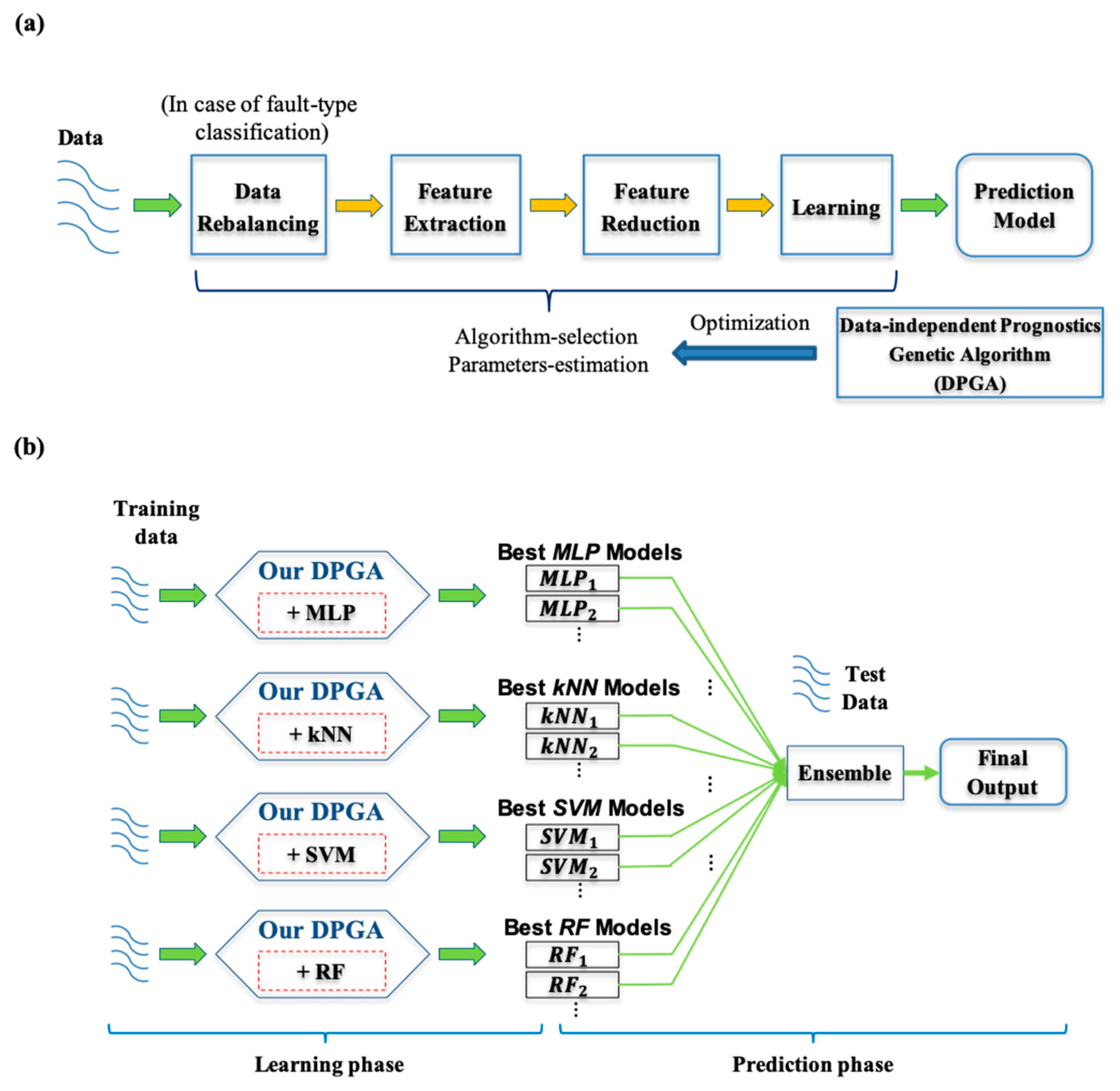
In this work, we propose a novel problem-independent framework for both the fault-type classification and the RUL prediction based on a GA. As we mentioned, the GA was employed to select the close-to-optimal set of data-processing algorithms and optimize the involved parameters in a robust way for a given dataset. As shown in Figure 1a, we first outlined the general process of the data-driven diagnostics and prognostics, which consists of four subtasks of data rebalancing (for classification problems), feature extraction, feature reduction, and learning. We did not explicitly include a feature selection in our framework, although it is a frequently used technique [48]. In fact, an implicit feature selection was already employed in the feature extraction stage because the inclusion and exclusion of created features are dynamically determined by a chromosome in the genetic algorithm (see the Section 3.1.1 for more details). As we explained in Section 2, a variety of algorithms in each subtask can be considered, and the diagnostics/prognostics performance is likely to be highly dependent on the selected algorithm and the specified parameter values. In this regard, it is necessary to select the optimal data preprocessing algorithms and specify the optimal parameter values involved by those algorithms. Hence, we propose a data-independent diagnostic/prognostic genetic algorithm (DPGA) to resolve it. In addition, our DPGA can be easily extended to generate an ensemble result [49,50] because it runs along with various learning methods, as shown in Figure 1b. We note that four representative machine-learning methods such as the multi-layer perceptron network (MLP), k-nearest neighbor (kNN), support vector machine (SVM), and random forest (RF) were employed in this study. As shown in Figure 1b, our DPGA runs to search the optimal data-processing algorithms for data rebalancing, feature extraction, and feature reduction subtasks and the relevant parameter values over the training dataset for each learning method in the learning phase. Then, a set of best solutions found by each DPGA are integrated into an ensemble to predict the fault-type or the RUL value over the test dataset in the prediction phase. In the following subsections, we explain the details of DPGA and the employed ensemble approach.

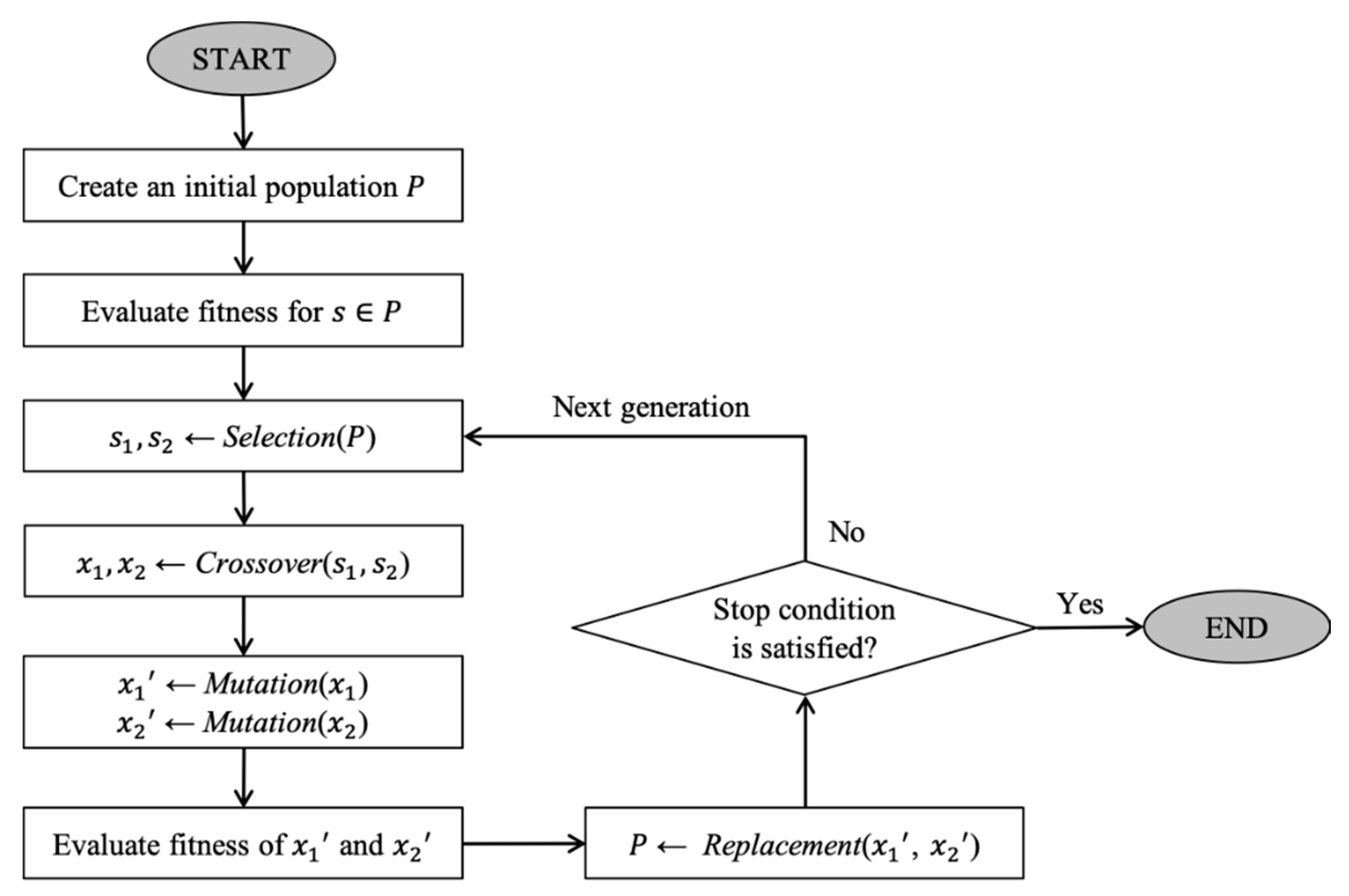
3.1. DPGA

DPGA is a steady-state genetic algorithm, and the overall framework is depicted in Figure 2. It first creates a random initial population of solutions, $P$, and evaluates the fitness of each solution. It selects two parent solutions $s_1$ and $s_2$ among the population according to the fitness values and generates two offspring solutions $x_1$ and $x_2$ by a crossover operation. These new solutions can be mutated with a low probability. After evaluating the fitness values of the offspring solutions, the GA replaces some old solutions in the population with them. This process is repeated until a stopping condition is satisfied. The specified values of parameters of the GA are summarized in

Table 1. Parameter values used in DPGA.

Parameters	Value
The number of solutions in a population $(\left|P\right|)$	20
Stopping-patience	50
The crossover probability ($p_c)$	0.5
The mutation probability ($p_m)$	0.1
The algorithm-change mutation probability	0.3
The parameter-change mutation probability	0.7

. In the following subsections, we introduce the details of each part in DPGA.

3.1.1. Chromosome Representation

In a GA, a solution is represented by a chromosome.

Table 2. Chromosome representation in DPGA. DR: Data rebalancing, FFE: Filtering-based feature extraction, RFE: Reduction-based feature extraction, LM: Learning model.

Field	Description	Range of Values
DR algo.	A data rebalancing algorithm	One of {None, RDUP, SMOTE, BSMOTE1, BSMOTE2, SSMOTE, RREM, NCL}
DR para.	A parameter value of the rebalancing algorithm	Balancing ratio $r$ $\in$ [0.75–1]
FFE algo.	A list of applied filtering-based feature extraction algorithms (Available only for time-series datasets)	A subset of {SMA, CMA, EMA, ES, LFS}
		(Note that the empty set means that no filtering-based feature extraction is applied.)
FFE para.	Parameter values of the applied filtering-based feature extraction algorithms	In case of SMA and CMA:
		The number of time points $n\in \left[3–10\right]$
		In case of LFS:
		Top χ% high-frequency components of the Fourier transform are removed, $\chi \in \left[10–50\right]$
		For EMA and ES:
		None
RFE algo.	A list of applied reduction-based feature extraction algorithms	A subset of {PCA,LSA,FAG,GRP,SRP}
		(Note that the empty set means that no reduction-based feature extraction is applied.)
RFE para.	Parameter values of the applied reduction-based feature extraction algorithms	In case of PCA, LSA, GRP, and SRP:
		The number of principal components $n_{PC}\in \left[1-max\left(\frac{\rho }{10},2\right)\right]$
		In case of FAG:
		The number of remaining features after merging $n_{FAG}\in \left[2-max\left(\frac{\rho }{10},3\right)\right]$
PCA flag	Indicator of whether or not the whole set of features is reduced by PCA	True or False
PCA para.	A parameter value to determine the number of dimensions reduced by PCA	The threshold amount of explained variance $ϵ$ $\in$ $\left[90–100\right]$
LM para.	Parameter values used for a specified learning algorithm	In case of MLP:
		The number of hidden neurons $n_{HN}\in \left[5–20\right]$
		The type of activation function $act{f}_{HL}\in \left\{tanh, relu\right\}$
		The type of optimization method $s{v}_{WO}\in \left\{lbfgs, adam\right\}$
		In case of kNN:
		The number of neighbors $n_{NN}\in \left[2–10\right]$
		The type of weight function $w{f}_{NN}\in \left\{uniform,distance\right\}$
		In case of SVM:
		The penalty parameter $C\in \left[1–8\right]$
		In case of RF:
		The number of trees $n_{tree}\in \left[2–10\right]$

shows a chromosome in DPGA, which is implemented by a one-dimensional list consisting of categorical and continuous variables to represent algorithm-selection and parameter-specification. Specifically, it is composed of four parts corresponding to data rebalancing, feature extraction, feature reduction, and learning subtasks as follows:

• Data rebalancing—This part is only applicable in the fault-types classification. As explained in Section 2.1, the ‘DR algo.’ field in a chromosome indicates one among five over-sampling and two under-sampling algorithms, or none of them. In addition, the ‘DR para.’ field represents the threshold parameter of the rebalancing ratio (see Section 2.1 for details).
• Feature extraction—To generate latent features, our GA employed two groups of approaches, filtering-based (available only for time-series datasets, see Section 2.2) and reduction-based (see Section 2.3) approaches. The ‘FFE algo.’ field represents the subset of five filtering-based feature extraction algorithms (SMA, CMA, EMA, ES, and LFS). In addition, the ‘FFE para.’ field includes the corresponding parameters that are necessary to run the selected feature extraction algorithms (for example, the number of time points in SMA or CMA). Similar to filtering-based feature extraction, the ‘RFE algo.’ and ‘RFE para.’ fields represent the combinatorial selection among five reduction-based feature extraction algorithms (PCA, LSA, FAG, GRP, and SRP) and the corresponding parameters (for example, the number of principal components), respectively. We note that if none are selected in ‘FFE algo.’ and ‘RFE algo.,’ only the original variables are used as input variables in the learning algorithm.
• Dimension-reduction by PCA—Before executing the learning method, the dimension of the input space consisting of all of the newly constructed features and the original variables can be finally reduced by the PCA [41,42,43]. The ‘PCA flag’ and ‘PCA para.’ represent whether PCA is applied or not, and the threshold parameter ($ϵ$) with respect to the desirable explained variance, respectively. In other words, when the ‘PCA flag’ turns on, the set of highest-order principal components that account for more than $ϵ\%$ of the data variability are selected as the final input variables to be fed into a learning method.
• Learning method: As explained before, we employed four machine-learning algorithms in this study. Therefore, the ‘LM para.’ field represents the corresponding parameters that are necessary to run the learning method as follows:

  -

  MLP: The MLP of a single hidden layer is assumed and $n_{HN}$ denotes the number of hidden nodes. In addition, the type of the activation function ($act{f}_{HL}$) is selected between the hyperbolic tan function (“tanh”) and the rectified linear unit function (“relu”). The solver for weight optimization ($s{v}_{WO}$) is also selected between an optimizer in the family of quasi-Newton methods (“lbfgs”) [51] and a stochastic gradient-based optimizer (“adam”) [52].

  -

  kNN: $n_{NN}$ denotes the number of nearest neighbors. In addition, the weight function ($w{f}_{NN}$) is selected between “uniform” and “distance.” In the former, the neighbors are weighted equally, whereas the neighbors are weighted by the inverse of the distance to the query in the latter.

  -

  SVM:$C$ denotes the penalty parameter for the misclassification.

  -

  RF: $n_{tree}$ denotes the number of trees in the forest.

3.1.2. Fitness Calculation

To evaluate a chromosome $s$, the F1-score and MSE measures (see Section 2.4 for details) are used for the fault-type classification and the RUL prediction, respectively, as follows.

$$fitness\left(s\right)=\{\begin{array}{ll}F1-macro\left(s\right)& \mathrm{for}fault-type\mathit{classification}\\ A- MSE\left(s\right)& \mathit{for}\mathit{RUL}\mathit{prediction}\end{array},$$

where $F1-macro\left(s\right)$ and $MSE\left(s\right)$ are the results by the leaning method using the algorithms and the parameter values included in $s$. In addition, $A$ denotes a constant large enough to make the fitness a positive real value. Consequently, the higher the fitness value, the better the solution in both the fault-type classification and the RUL prediction problems. To avoid the over-fitting, we used $d$-fold cross-validation in computing the fitness over the training data. More specifically, the whole training dataset was randomly divided into $d$ disjoint subsets. Then, each subset was held out for evaluation while the rest $\left(d-1\right)$ of the subsets were used as the training data. For a more stable fitness evaluation, we repeated the cross-validation $l$ times. Accordingly, the fitness of $s$ is the average over $d \times l$ trials. In this work, we set $d$ to 5 and $l$ to 3.

3.1.3. Selection

To choose a parent solution from the population $P$, we employed the roulette wheel selection where the selection probability of a chromosome $x$ is proportional to the fitness value of $x$ as follows:

$$\mathrm{Pr}\left(x\right)=\frac{fitness\left(x\right)}{{{\displaystyle \sum }}_{y\in P}fitness\left(y\right)}.$$

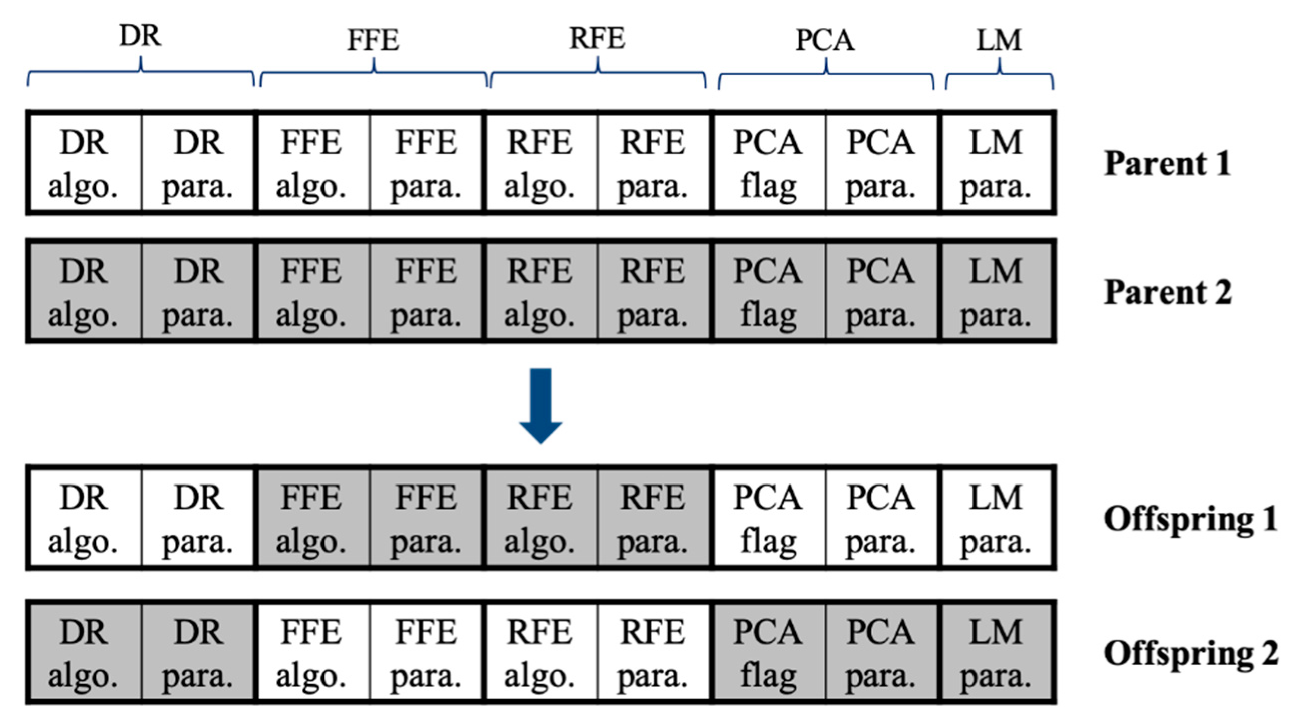
3.1.4. Crossover

Two new offspring solutions are generated by a crossover with a probability $p_c$, or they are duplicated from the parent solutions with a probability $1-p_c$. The employed crossover is a block-wise uniform crossover, as shown in Figure 3. Specifically, there are five blocks such as ‘DR,’ ‘FFE,’ ‘RFE,’ ‘PCA,’ and ‘LM,’ all of which, except for the last block, consist of ‘algo. (or flag)’ and ‘para.’ fields, as explained in Section 3.1.1. For each block, the first offspring chromosome is inherited from one of two parent chromosomes uniformly at random and the second offspring chromosome is inherited from the remaining parent chromosome. For example, the first offspring inherited DR, PCA, and LM blocks from the first parent, whereas FFE and RFE blocks were inherited from the second parent in Figure 3.

3.1.5. Mutation

The offspring chromosome created by the block-wise crossover is mutated with a small probability $p_m$, whereas the offspring created by the duplication is surely mutated to create a new chromosome that is not identical to the parent chromosome. Only one among four blocks, ‘DR,’ ‘FFE,’ ‘RFE,’ and ‘PCA,’ in the offspring is randomly selected, and it is mutated by one of the following two ways:

• Algorithm-change mutation—The selected algorithm is changed. In other words, the current choice in the ‘DR algo.’, ‘FFE algo.’, ‘RFE algo.’, or ‘PCA flag’ field is replaced with an alternative uniformly at random.
• Parameter-change mutation—The parameter value specified for the corresponding algorithm is mutated. In other words, the ‘DR para.’, ‘FFE para.’, ‘RFE para.’, or ‘PCA para’ field is replaced with a new value.

In this work, the parameter-change mutation probability was set to a larger value (0.7) than the algorithm-change mutation probability (0.3) considering that the range of values in the former case is much wider than that in the latter case.

3.1.6. Replacement and Stop Criterion

When the offspring solution is better than the worst solution in the population, the latter is replaced with the former. For an efficient stopping criterion, we set a patience parameter $T$. Our GA stops when the best solution in the population is not improved during the past $T$ consecutive generations.

3.2. Ensemble Methods

As explained in Figure 1b, the DPGA can produce many prediction models, which can constitute an ensemble of solutions. Herein, we employed the voting ensemble and the Kalman filter ensemble [53] for the fault-type classification and the RUL prediction, respectively. For the former case, we applied a soft voting rule to achieve the combined results of multiple optimal classifiers. The voting ensemble is based on the sums of the predicted probabilities from well-calibrated classifiers. The Kalman filter ensemble can provide a mechanism for fusing multiple model predictions over time for a stable and high prediction performance.

4. Results

To validate the performance of our method, we compared it to the traditional grid-search approaches over the following two fault-type classification benchmark datasets and one RUL prediction benchmark dataset.

4.1. Datasets

4.1.1. Steel Plates Faults Dataset

This dataset is provided by the Semeion Research Center of Sciences of Communication (www.semeion.it). Each observation is classified into seven different types of steel plate’s faults, namely, Pastry, Z-Scratch, K-Scratch, Stains, Dirtiness, Bumps, and Other Faults [54,55]. The numbers of observations corresponding to the fault type are shown in

Table 3. Steel plates faults dataset.

Class	Type of Faults	Number of Observations
1	Pastry	158
2	Z-Scratch	190
3	K-Scratch	391
4	Stains	72
5	Dirtiness	55
6	Bumps	402
7	Other Faults	673

. As shown in the table, the numbers of observations vary a lot from one category to another. The total number of observations is 1941, and each observation is made up of 27 features representing the geometric shape of the defect and its contour.

4.1.2. SECOM Dataset

The dataset provided by UCI Machine Learning Repository (http://archive.ics.uci.edu/mL) is related to a semiconductor manufacturing process. The dataset consists of 1567 observations, and each observation is made up of 591 features representing manufacturing operations of a single semiconductor [56]. The data were collected from the continuous monitoring process using sensors and metrology equipment along the semiconductor manufacturing line. At the end of manufacturing operation, functional testing was performed to ensure that the semiconductor meets the specification for which it is designed. If the result met the expectation, the semiconductor would be classified as the accepted product; otherwise, it would be rejected. There are only 104 rejected cases, whereas there are 1463 accepted cases. Due to its high imbalance ratio, it is difficult to get a high classification performance on the dataset.

4.1.3. NASA C-MAPSS Dataset

The NASA commercial modular aero-propulsion system simulation (C-MAPSS) dataset is generated by using a model-based simulation program [57,58]. It is further divided into four sub-datasets, as shown in

Table 4. NASA C-MAPSS dataset details.

Sub-Dataset	FD001	FD002	FD003	FD004
Train trajectories	100	260	100	248
Test trajectories	100	259	100	248
No. of operational modes	1	6	1	6

. Each trajectory within the train and test trajectories is assumed to be the life-cycle of an aircraft gas turbine engine, and starts with different degrees of initial wear and manufacturing variation, which are unknown to the data analyzer. All engines operate in normal condition at the start, and then begin to degrade at some point. The degradation in the training set grows in magnitude until failure, while the degradation in the test set ends prior to failure. Thus, the main objective is to predict the correct RUL value for each engine in the test set.

The data are arranged in an $N$-by-26 matrix where $N$ corresponds to the number of data points in each dataset. Each row is a snapshot taken during a single operational cycle and includes 26 different features: Engine number, time step (in cycles), three operational settings, and 21 sensor measurements (temperature, pressure, fan/core speed, and so on). The three features of operational settings specify the flight condition or operational mode of an engine, which have a substantial effect on engine performance [53,59,60]. There is a single operational mode in FD001 and FD003 sub-datasets, whereas there are six operational modes in FD002 and FD004 sub-datasets. Therefore, the operational mode was included as a feature by using six real variables, each of which represents the number of cycles spent in the corresponding operational mode since the beginning of the series [53]. In addition, they were normalized as in [53].

4.2. Performance Comparisons between DPGA and Grid-Search Approaches

We compare the prediction performance of our method to the traditional exhaustive grid-search (EGS) approaches applied to MLP, kNN, SVM, and RF (we call them EGS-MLP, EGS-kNN, EGS-SVM, and EGS-RF, respectively). In an EGS approach, 5-fold cross-validation is conducted to find an optimal set of parameters. In addition, we further compared the performance of the ensemble of the prediction models of all EGS approaches (we call this EGS-E). As our method, the voting ensemble and the Kalman filter ensemble for the fault-type classification and the RUL prediction, respectively, were used for EGS-E. We first scatter-plotted the relation of the performance between the training and test sets by DPGA and five EGS approaches (Figure 4). Unfortunately, the positive relation was not observed among the results of EGS approaches in all figures. This implies that a better solution in the training set can show a worse performance over the test set. Therefore, it is not efficient to simply select a best grid-search approach based on the training set. Interestingly, our approach (DPGA) was best over the test set, whereas it was not best over the training set in all datasets. Figure 5 shows the result where Y-axis values mean the average and the standard deviation of the F1-score or MSE values in the test dataset over 50 trials. As shown in the figure, our DPGA achieved significantly better results among the examined methods in all datasets of fault-type classification and the RUL prediction problems (all p-values < 0.02). Specifically, the second-best methods were EGS-kNN, EGS-E, and EGS-MLP for the C-MAPSS, steel-plate, and SECOM datasets, respectively. This implies that the performance of a learning algorithm is varied across the given dataset, but our method stably overwhelmed the EGS approaches. In addition, we investigated the best solutions found by EGS (

Table 5. Best solutions found by the exhaustive grid-search approaches (NA: Not available).

Dataset	Method	DR	FFE	RFE	PCA	Parameters
FD001	EGS-MLP	NA	ES	None	False	$s{v}_{WO}=lbfgs, n_{HN}=20, act{f}_{HL}=relu$
	EGS-kNN	NA	SMA	None	False	$n_{NN}=4, w{f}_{NN}=distance$
	EGS-SVM	NA	ES	None	False	$C=8$
	EGS-RF	NA	ES	None	False	$n_{tree}=10$
FD002	EGS-MLP	NA	ES	None	False	$s{v}_{WO}=adam, n_{HN}=18, act{f}_{HL}=tanh$
	EGS-kNN	NA	EMA	None	False	$n_{NN}=10, w{f}_{NN}=distance$
	EGS-SVM	NA	ES	None	False	$C=6$
	EGS-RF	NA	ES	None	False	$n_{tree}=10$
FD003	EGS-MLP	NA	ES	None	False	$s{v}_{WO}=lbfgs, n_{HN}=20, act{f}_{HL}=relu$
	EGS-kNN	NA	SMA	None	False	$n_{NN}=8, w{f}_{NN}=distance$
	EGS-SVM	NA	ES	None	False	$C=8$
	EGS-RF	NA	ES	None	False	$n_{tree}=6$
FD004	EGS-MLP	NA	ES	None	False	$s{v}_{WO}=lbfgs, n_{HN}=15, act{f}_{HL}=relu$
	EGS-kNN	NA	None	None	False	$n_{NN}=10, w{f}_{NN}=distance$
	EGS-SVM	NA	ES	None	False	$C=8$
	EGS-RF	NA	ES	None	False	$n_{tree}=10$
Steel plates faults	EGS-MLP	NCL	None	None	False	$r=1.0, s{v}_{WO}=adam, n_{HN}=15, act{f}_{HL}=tanh$
	EGS-kNN	None	None	None	False	$n_{NN}=8, w{f}_{NN}=distance$
	EGS-SVM	NCL	None	None	False	$r=1.0, C=4$
	EGS-RF	SSMOTE	None	None	False	$r=1.0, n_{tree}=10$
SECOM	EGS-MLP	RDUP	None	None	False	$r=1.0, s{v}_{WO}=adam, n_{HN}=20, act{f}_{HL}=relu$
	EGS-kNN	RDUP	None	None	False	$r=1.0, n_{NN}=2, w{f}_{NN}=uniform$
	EGS-SVM	SSMOTE	None	None	False	$r=1.0, C=8$
	EGS-RF	SMOTE	None	None	False	$r=1.0, n_{tree}=8$

) and DPGA (

Table 6. Best solutions of our DPGA approach in RUL prediction datasets. (a–d) Results of the sub-dataset FD001, FD002, FD003, and FD004, respectively, in the NASA C-MAPSS dataset. Bold values denote the minority cases in all sub-datasets.

(a) FD001 dataset
FFE Algo.	FFE Para.	RFE Algo.	RFE Para.	PCA Flag	PCA Para.	LM Para.
CMA	$n_{MA}=10$	PCA, LSA	$n_{PC}=1$	TRUE	$ϵ=91.649$	MLP: $s{v}_{WO}=adam\wedge n_{HN}=11\wedge act{f}_{HL}=tanh$
CMA	$n_{MA}=10$	LSA, FAG	$n_{FAG}=2$ $n_{PC}=1$	TRUE	$ϵ=91.649$	MLP: $s{v}_{WO}=adam\wedge n_{HN}=11\wedge act{f}_{HL}=tanh$
CMA	$n_{MA}=10$	LSA, FAG	$n_{FAG}=2$ $n_{PC}=1$	TRUE	$ϵ=91.649$	MLP: $s{v}_{WO}=adam\wedge n_{HN}=10\wedge act{f}_{HL}=tanh$
SMA, CMA, EMA, ES	$n_{MA}=10$	PCA, LSA	$n_{PC}=1$	TRUE	$ϵ=98.517$	kNN: $n_{NN}=7\wedge w{f}_{NN}=uniform$
CMA, EMA, ES, LFS	$n_{MA}=6$ $\chi =40.196$	PCA	$n_{PC}=1$	TRUE	$ϵ=98.394$	kNN: $n_{NN}=9\wedge w{f}_{NN}=distance$
CMA, ES	$n_{MA}=6$	None	None	TRUE	$ϵ=99.012$	SVM: $C=5$
CMA, ES	$n_{MA}=9$	FAG	$n_{FAG}=2$	TRUE	$ϵ=99.477$	RF: $n_{tree}=4$
(b) FD002 dataset
FFE Algo.	FFE Para.	RFE Algo.	RFE Para.	PCA Flag	PCA Para.	LM Para.
SMA, CMA, EMA	$n_{MA}=4$	PCA, LSA, FAG, GRP	$n_{FAG}=2$ $n_{PC}=2$	TRUE	$ϵ=99.456$	MLP: $s{v}_{WO}=adam\wedge n_{HN}=6\wedge act{f}_{HL}=relu$
CMA	$n_{MA}=9$	FAG	$n_{FAG}=3$	TRUE	$ϵ=99.980$	kNN: $n_{NN}=5\wedge w{f}_{NN}=uniform$
CMA	$n_{MA}=10$	PCA	$n_{PC}=1$	TRUE	$ϵ=98.771$	SVM: $C=4$
CMA	$n_{MA}=9$	PCA	$n_{PC}=1$	TRUE	$ϵ=98.771$	SVM: $C=4$
SMA, EMA	$n_{MA}=10$	PCA, LSA, FAG, GRP, SRP	$n_{FAG}=3$ $n_{PC}=2$	TRUE	$ϵ=93.179$	RF: $n_{tree}=5$
SMA, CMA	$n_{MA}=9$	PCA	$n_{PC}=2$	TRUE	$ϵ=93.179$	RF: $n_{tree}=5$
(c) FD003 dataset
FFE Algo.	FFE Para.	RFE Algo.	RFE Para.	PCA Flag	PCA Para.	LM Para.
SMA, CMA, ES	$n_{MA}=10$	LSA, GRP	$n_{PC}=1$	TRUE	$ϵ=94.131$	MLP: $s{v}_{WO}=adam\wedge n_{HN}=8\wedge act{f}_{HL}=relu$
CMA, ES, LFS	$\chi =21.056$ $n_{MA}=9$	LSA	$n_{PC}=2$	TRUE	$ϵ=95.048$	kNN: $n_{NN}=7\wedge w{f}_{NN}=uniform$
SMA, ES	$n_{MA}=8$	PCA, LSA, FAG	$n_{PC}=1$ $n_{FAG}=2$	TRUE	$ϵ=95.047$	SVM: $C=4$
SMA, ES	$n_{MA}=8$	PCA, LSA, FAG	$n_{PC}=1$ $n_{FAG}=2$	TRUE	$ϵ=93.092$	SVM: $C=4$
SMA, CMA, EMA, ES	$n_{MA}=9$	FAG, SRP	$n_{PC}=1$ $n_{FAG}=2$	TRUE	$ϵ=96.689$	RF: $n_{tree}=8$
(d) FD004 dataset
FFE Algo.	FFE Para.	RFE Algo.	RFE Para.	PCA Flag	PCA Para.	LM Para.
EMA	None	PCA, FAG	$n_{FAG}=3$ $n_{PC}=1$	TRUE	$ϵ=92.148$	MLP: $s{v}_{WO}=adam\wedge n_{HN}=6\wedge act{f}_{HL}=relu$
CMA	$n_{MA}=10$	FAG	$n_{FAG}=2$	TRUE	$ϵ=99.023$	kNN: $n_{NN}=5\wedge w{f}_{NN}=distance$
SMA, EMA, LFS	$n_{MA}=10$ $\chi =23.091$	FAG	$n_{FAG}=2$	TRUE	$ϵ=99.987$	SVM: $C=4$
SMA, EMA, LFS	$n_{MA}=9$ $\chi =23.091$	FAG	$n_{FAG}=2$	TRUE	$ϵ=99.987$	SVM: $C=4$
LFS	$\chi =45.570$	PCA, LSA	$n_{PC}=2$	TRUE	$ϵ=99.825$	RF: $n_{tree}=5$

and

Table 7. Best solutions of our DPGA approach in fault-types classification datasets. (a,b) Results of the steel plates faults and SECOM datasets, respectively.

(a) Steel plates faults dataset
DR Algo.	DR Para.	RFE Algo.	RFE Para.	PCA Flag	PCA Para.	LM Para.
SSMOTE	$r_{2m}=0.934$	FAG	$n_{FAG}=2$	TRUE	$ϵ=98.964$	MLP: $s{v}_{WO}=adam\wedge n_{HN}=20\wedge act{f}_{HL}=tanh$
SMOTE	$r_{2m}=0.933$	FAG	$n_{FAG}=3$	TRUE	$ϵ=98.964$	MLP: $s{v}_{WO}=adam\wedge n_{HN}=19\wedge act{f}_{HL}=tanh$
SMOTE	$r_{2m}=1$	PCA	$n_{PC}=1$	TRUE	$ϵ=93.742$	kNN: $n_{NN}=2\wedge w{f}_{NN}=distance$
BSMOTE1	$r_{2m}=0.918$	PCA	$n_{PC}=1$	TRUE	$ϵ=93.742$	kNN: $n_{NN}=3\wedge w{f}_{NN}=distance$
RDUP	$r_{2m}=0.834$	PCA	$n_{PC}=1$	TRUE	$ϵ=93.742$	kNN: $n_{NN}=3\wedge w{f}_{NN}=distance$
SMOTE	$r_{2m}=0.928$	PCA, LSA, FAG	$n_{PC}=2$ $n_{FAG}=2$	TRUE	$ϵ=98.157$	SVM: $C=7$
BSMOTE1	$r_{2m}=1$	PCA, LSA, FAG	$n_{PC}=1$ $n_{FAG}=3$	TRUE	$ϵ=98.634$	SVM: $C=8$
RDUP	$r_{2m}=0.931$	PCA, LSA	$n_{PC}=1$	TRUE	$ϵ=98.216$	RF: $n_{tree}=9$
BSMOTE1	$r_{2m}=0.993$	PCA, LSA, FAG	$n_{PC}=1$ $n_{FAG}=3$	TRUE	$ϵ=98.859$	RF: $n_{tree}=10$
RDUP	$r_{2m}=0.874$	FAG	$n_{FAG}=3$	TRUE	$ϵ=98.216$	RF: $n_{tree}=10$
(b) SECOM dataset
DR Algo.	DR Para.	RFE Algo.	RFE Para.	PCA Flag	PCA Para.	LM Para.
BSMOTE1	$r_{2m}=0.910$	LSA, FAG	$n_{PC}=53$ $n_{FAG}=52$	TRUE	$ϵ=97.867$	MLP: $s{v}_{WO}=adam\wedge n_{HN}=20\wedge act{f}_{HL}=relu$
RDUP	$r_{2m}=0.907$	LSA, FAG	$n_{PC}=54$ $n_{FAG}=52$	TRUE	$ϵ=96.521$	MLP: $s{v}_{WO}=adam\wedge n_{HN}=17\wedge act{f}_{HL}=relu$
RDUP	$r_{2m}=0.910$	None	None	TRUE	$ϵ=98.027$	kNN: $n_{NN}=2\wedge w{f}_{NN}=distance$
RDUP	$r_{2m}=0.763$	None	None	TRUE	$ϵ=97.678$	kNN: $n_{NN}=2\wedge w{f}_{NN}=uniform$
BSMOTE2	$r_{2m}=0.968$	PCA, LSA, FAG	$n_{PC}=8$ $n_{FAG}=20$	TRUE	$ϵ=98.322$	SVM: $C=6$
SSMOTE	$r_{2m}=0.803$	FAG	$n_{FAG}=19$	TRUE	$ϵ=90.882$	RF: $n_{tree}=9$
SMOTE	$r_{2m}=0.934$	LSA	$n_{PC}=9$	TRUE	$ϵ=91.980$	RF: $n_{tree}=9$

), and observed that they are very different to each other. EGS approaches have almost found the best solution, which only includes an algorithm of the FFE (filter-based feature extraction) part and the RD (rebalancing data) part in the RUL prediction and the fault-type classification, respectively. In other words, the RFE and the PCA part were not useful in the search. On the other hand, the best solutions found by DPGA have included valid algorithms in all RD, FFE, RFE, and PCA parts. Specifically, the RD (in fault-type classification), FFE (in RUL prediction), and PCA parts were effective in all best-found solutions. This means that DPGA has efficiently searched a variety of combinations of all subtasks in the fault-type classification and the RUL prediction.

Finally, we compare the running time between the approaches on a system with a four-core Intel^® Core™ i7-6700 Processor 3.40 GHz and 16 GB of memory. As the execution time of the Kalman filter or voting ensemble is very small (less than 1 min), we compared the running time of DPGA to that of EGS-E only (Figure 6). Note that the running time is measured for the learning phase in Figure 1b. As shown in the figure, the running time of DPGA is even shorter than that of the EGS-E for the small-sized dataset (steel plates faults). For large datasets (FD001–FD004, and SECOM), the running time of DPGA approaches was, at most, 1.9 times longer than that of the EGS-E ones, which is practically acceptable considering the performance improvement.

5. Conclusions

In this study, we proposed a DPGA, which is a novel framework to predict the RUL and fault-types. It is a self-adaptive method to select the close-to-optimal set of data-preprocessing algorithms and optimize the involved parameters in each subtask of data rebalancing, feature extraction, feature reduction, and learning. Although DPGA used four machine-learning methods such as the multi-layer perceptron network, k-nearest neighbor, support vector machine, and random forest in this study, it can be easily extended to combine other kinds of machine-learning methods. In addition, our method seems robust because it can generate an ensemble of prediction models. Through the performance comparison of DPGA with the traditional grid-search framework over three benchmark datasets, the former showed significantly better accuracies than the latter in a comparable running time. This implies that our genetic search was efficient in solving the large-scaled diagnostics and prognostics problems. It was interesting that the best solutions found by DPGA involve many filtering- or reduction-based feature extraction algorithms to generate various feature variables. As shown in the results, it is advantageous that DPGA can be applicable to other machinery systems without a priori knowledge about the most proper machine-learning method or a feature processing algorithm. In a future study, a parallel and distributed version of the DPGA method can be developed to reduce the execution time. It is also promising to further validate the usefulness of our approach by employing other kinds of the machine-learning models such as the recurrent neural network. Finally, it will be another interesting future study to design a more robust ensemble approach than what was employed in DPGA.