Article

A Remote-Sensing Method to Estimate Bulk Refractive Index of Suspended Particles from GOCI Satellite Measurements over Bohai Sea and Yellow Sea

1
School of Marine Sciences, Nanjing University of Information Science & Technology, Nanjing 210044, China
2
Jiangsu Research Center for Ocean Survey Technology, Nanjing University of Information Science & Technology, Nanjing 210044, China
3
Chuzhou Meteorological Bureau, Chuzhou 239000, China
4
State Key Laboratory of Satellite Ocean Environment Dynamics, Second Institute of Oceanography, Ministry of Natural Resources, Hangzhou 310012, China
*
Author to whom correspondence should be addressed.
Appl. Sci. 2020, 10(1), 23; https://doi.org/10.3390/app10010023
Submission received: 22 November 2019 / Revised: 12 December 2019 / Accepted: 15 December 2019 / Published: 18 December 2019
(This article belongs to the Special Issue Remote Sensing and Geoscience Information Systems in Applied Sciences)

Abstract

:

Featured Application

The study proposed a multiple-step hybrid remote sensing method to estimate bulk refractive index (np) of suspended particles in the Bohai Sea and Yellow Sea from GOCI satellite measurements. This proposed method can be applied to study the spatial and temporal variations of np in the Bohai Sea and Yellow Sea, and thereby to understand the particulate biogeochemical properties (e.g., composition and size) and their role in exploring the changes of marine environments.

Abstract

The bulk refractive index (np) of suspended particles, an apparent measure of particulate refraction capability and yet an essential element of particulate compositions and optical properties, is a critical indicator that helps understand many biogeochemical processes and ecosystems in marine waters. Remote estimation of np remains a very challenging task. Here, a multiple-step hybrid model is developed to estimate the np in the Bohai Sea (BS) and Yellow Sea (YS) through obtaining two key intermediate parameters (i.e., particulate backscattering ratio, Bp, and particle size distribution (PSD) slope, j) from remote-sensing reflectance, Rrs(λ). The in situ observed datasets available to us were collected from four cruise surveys during a period from 2014 to 2017 in the BS and YS, covering beam attenuation (cp), scattering (bp), and backscattering (bbp) coefficients, total suspended matter (TSM) concentrations, and Rrs(λ). Based on those in situ observation data, two retrieval algorithms for TSM and bbp were firstly established from Rrs(λ), and then close empirical relationships between cp and bp with TSM could be constructed to determine the Bp and j parameters. The series of steps for the np estimation model proposed in this study can be summarized as follows: Rrs (λ) → TSM and bbp, TSM → bpcpj, bbp and bpBp, and j and Bpnp. This method shows a high degree of fit (R2 = 0.85) between the measured and modeled np by validation, with low predictive errors (such as a mean relative error, MRE, of 2.55%), while satellite-derived results also reveal good performance (R2 = 0.95, MRE = 2.32%). A spatial distribution pattern of np in January 2017 derived from GOCI (Geostationary Ocean Color Imager) data agrees well with those in situ observations. This also verifies the satisfactory performance of our developed np estimation model. Applying this model to GOCI data for one year (from December 2014 to November 2015), we document the np spatial distribution patterns at different time scales (such as monthly, seasonal, and annual scales) for the first time in the study areas. While the applicability of our developed method to other water areas is unknown, our findings in the current study demonstrate that the method presented here can serve as a proof-of-concept template to remotely estimate np in other coastal optically complex water bodies.

1. Introduction

The bulk refractive index (np) of suspended particles in natural waters is a critical physical parameter that describes particulate intrinsic properties such as material composition, shape, texture, and structure [1,2,3,4,5]. This parameter carries much critical information that significantly supports the research on the underwater light properties of particulate assemblages, and it is closely related to many marine ecological and biogeochemical processes and is, thus, capable of contributing to the knowledge of regional and even global ocean ecosystems [4,6]. Consequently, acquiring np information, such as its spatiotemporal distribution, is of great significance to us.
At present, several measurement methods for the bulk refractive index of suspended particles are available to us, such as the laser diffraction method, electrical resistance technique, and flow cytometry analysis [7,8,9]. These methods show relatively high observational accuracy and yet are time-consuming and laborious and need a large quantity of water sample collections. More importantly, they struggle to provide variations in large-scale synoptic and temporal distributions. Actually, the np data records remain scarce, especially for large-scale marine waters. The remote sensing technique provides a possibility for filling this gap.
A large quantity of algorithms was developed for remote sensing estimation on water condition parameters such as chlorophyll a [10,11,12,13,14], suspended particulate matter [15,16,17], turbidity [18,19], and even colored dissolved organic matter [20,21,22]. However, it is unfortunate that fewer algorithms were developed to derive the bulk refractive index of suspended particles. Based on the Twardowski et al. (2001) [2] model, i.e., modeling the np using the particulate backscattering ratio (Bp) and hyperbolic slope of the particle size distribution (j), Suresh et al. (2006) [23] developed an empirical band ratio method to model Bp and j and then further estimated the np in the Arabian Sea from Remote Sensing Satellite (IRS-P4), Ocean Color Monitor (OCM)satellite data. They found that the np values were low in the open ocean and relatively high in the coastal waters. Based on Mie theory, Nasiha et al. (2014) [4] developed a retrieval model to estimate the np to understand particulate assemblage dynamics in coastal waters. To apply this inversion model to satellite data, Nasiha et al. (2015) [5] further proposed a proof-of-concept method to derive the np from Moderate-Resolution Imagine Spectroradiometer (MODIS)-Aqua images. This method firstly uses an empirical relationship to estimate turbidity based on single green band (551 nm) reflectance and then deduces the parameters, including Bp, j, and particulate apparent density (ρa), which are finally used to calculate the refraction index.
Clearly, the np estimation models using remotely sensed data remain very limited. Additionally, the existing methods are mostly based on empirical relationships such as those between Rrs(λ) band ratios with the parameters Bp and j of Suresh et al., (2006) [23] and fitted empirical relationships between Rrs(λ) with turbidity and Bp [5]. Although case studies showed good performance, the lack of a necessary physical basis still limits the use of these methods, despite their proof of concept. Therefore, more validation should be undertaken to evaluate the previous limited methods for application to other water areas of interest. Importantly, new np estimation models should be developed to cope with different water conditions, especially for turbid coastal waters.
This study collects an adequate bio-optical dataset that covers the measurements of inherent optical properties, such as particulate backscattering (bbp), scattering (bp), and beam attenuation (cp) coefficients, remote sensing reflectance (Rrs(λ)) measurement, and total suspended matter (TSM) measurement. The investigated water areas of this study were the Bohai Sea and Yellow Sea. The objective of the current study was to develop a method for remote sensing estimation of np by using satellite ocean color data. This study proposes a multiple-step hybrid model that firstly depends on the TSM and bbp retrievals, then the established close relationships between bp and cp with TSM, and ultimately upon the Twardowski et al. (2001) [2] model derived from Mie theory calculations. By using independent datasets including in situ data and satellite retrievals, the proposed method is assessed, and then applied to Geostationary Ocean Color Imager (GOCI) data. The spatiotemporal distribution patterns of np are documented. At last, some necessary discussions are appended.

2. Data and Methods

2.1. The Study Water Areas

The investigated water areas of this study were the marginal seas of the northwest Pacific Ocean along with China, i.e., the Bohai Sea (BS) and Yellow Sea (YS). The BS and YS are typically large shallow semi-enclosed seas with a water depth from several meters to about 100 m (Figure 1). These seas are highly turbid and optically complex waters that are significantly influenced by terrigenous discharge. The datasets used in the present study were collected from four cruise surveys in November 2014, August 2015, July 2016, and January 2017 in the BS and YS (Figure 1).

2.2. Bio-Optical Measurements
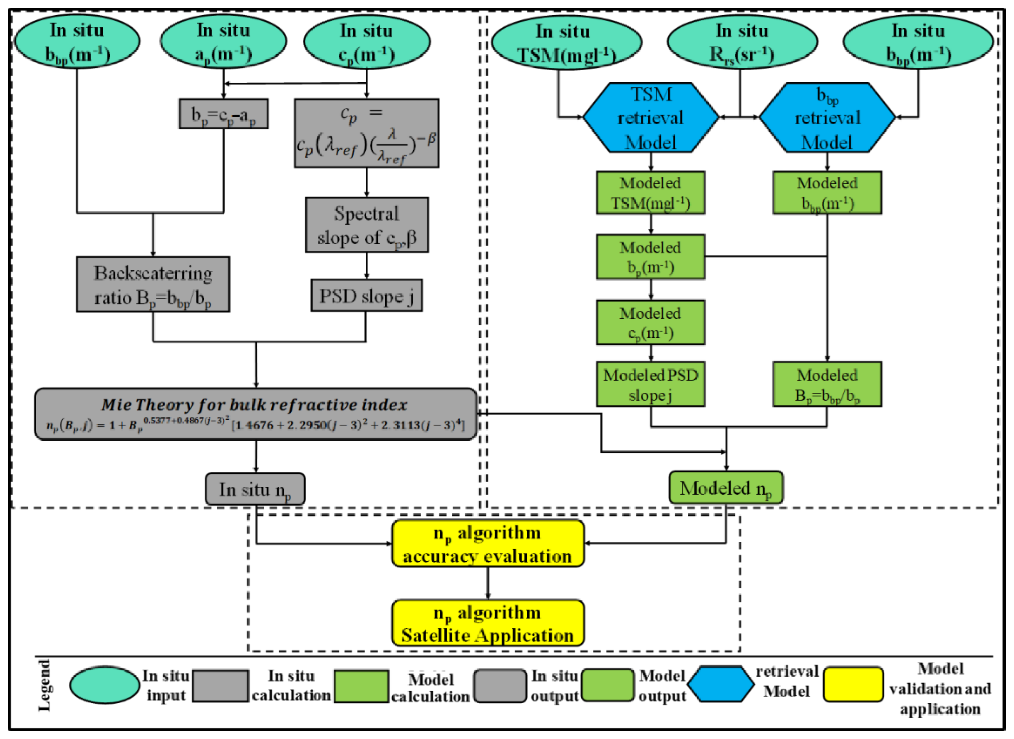
By using a profiling package, bio-optical measurements were performed to measure various optical parameters. The package included a Seabird ABE911P conductivity–temperature–depth (CTD) profiler that was used to measure hydrological characteristics of the water bodies and some optical devices, including a WET Labs AC-S and a HOBI Labs Hydroscat-6 (HS-6). The particulate absorption coefficient (ap(λ)) and beam attenuation coefficient (cp(λ)) in the spectral range of 400–700 nm were observed with the AC-S instrument, and then the particulate scattering coefficient (bp(λ)) could be derived using the relationship bp(λ) = cp(λ) − ap(λ). The particulate backscattering coefficient, bbp(λ), was observed by the HS-6 instrument which has six spectral channels, i.e., 442, 488, 550, 620, 700, and 852 nm, while the blue and green bands (i.e., 442, 488, and 550 nm) were used as delegates for the analysis in this study. The detailed measurement methods for the AC-S and HS-6 instruments can be seen in the Sun et al. (2016) [24] study.
The remote sensing reflectance (Rrs(λ)) spectra were collected with a Satlantic Hyper-Profiler II radiometer [25]. Meanwhile, water samples were simultaneously collected along with the above optical measurements and then filtered immediately in the lab onboard. The filtered particulates on GF/F filters were used to analyze total suspended matter (TSM) concentrations [24]. The collected bio-optical parameters during the four cruises are summarized in Table 1.

2.3. np Calculation

The bulk refractive index of suspended particles (np) was calculated using a Mie theory-based relationship model from the so-called input parameters, namely, the particulate backscattering ratio BP and the particle size distribution (PSD) slope j (Equation (1) by Twardowski et al., (2001) [2]).
n p = 1 + B p 0.5377 + 0.4867 ( j 3 ) 2 [ 1.4676 + 2.2950 ( j 3 ) 2 + 2.3113 ( j 3 ) 4 ] .
Here, the Bp (=bbp/bp), bbp, and bp were measured by HS-6 and AC-S. The cp(λ) spectrum can be modeled using a hyperbolic power function [2,26,27].
c p ( λ ) = c p ( λ ref ) × ( λ λ ref ) β ,
where λref is a reference wavelength, and β is the spectral slope parameter. By using the cp at different wavelengths, we were accordingly able to calculate parameter β. According to Boss et al. [28], the parameter β is found to covary with the parameter j, which can be refined as the following equation for more PSD cases:
j = β + 3 0.5 e 6 β .
Therefore, we can obtain the parameter j to calculate the np.

2.4. GOCI Data Collection and Processing

In this study, GOCI Level-1B data were used to assess the application of the developed refractive index (np) model. As a geostationary ocean color remote sensing satellite, GOCI receives images eight times a day from 12:15 a.m. to 7:45 a.m. Greenwich Mean Time (GMT) (8:15 to 15:15 local time) with 1-h temporal resolution. The GOCI satellite data have a spatial coverage of about 2500 km × 2500 km covering the northwest Pacific Ocean, a spatial resolution of 500 m, and eight spectral bands with the central wavelengths of 412, 443, 490, 555, 660, 680, 745, and 865 nm. In this study, a total of 2825 GOCI satellite images during the one-year period from December 2014 to November 2015 were downloaded from the Korea Ocean Satellite Center (KOSC). By utilizing the GOCI Data Processing System (GDPS, version 1.3), the image data focusing on the BS and YS regions were firstly extracted and then processed by the default atmospheric correction method of Wang & Gordon (1994) [29] to output Rrs(λ) data. These Rrs(λ) data were further quality controlled by using the various flags such as stray light and cloud coverage to avoid interference from invalid satellite data signals.

2.5. Development of np Estimation Model

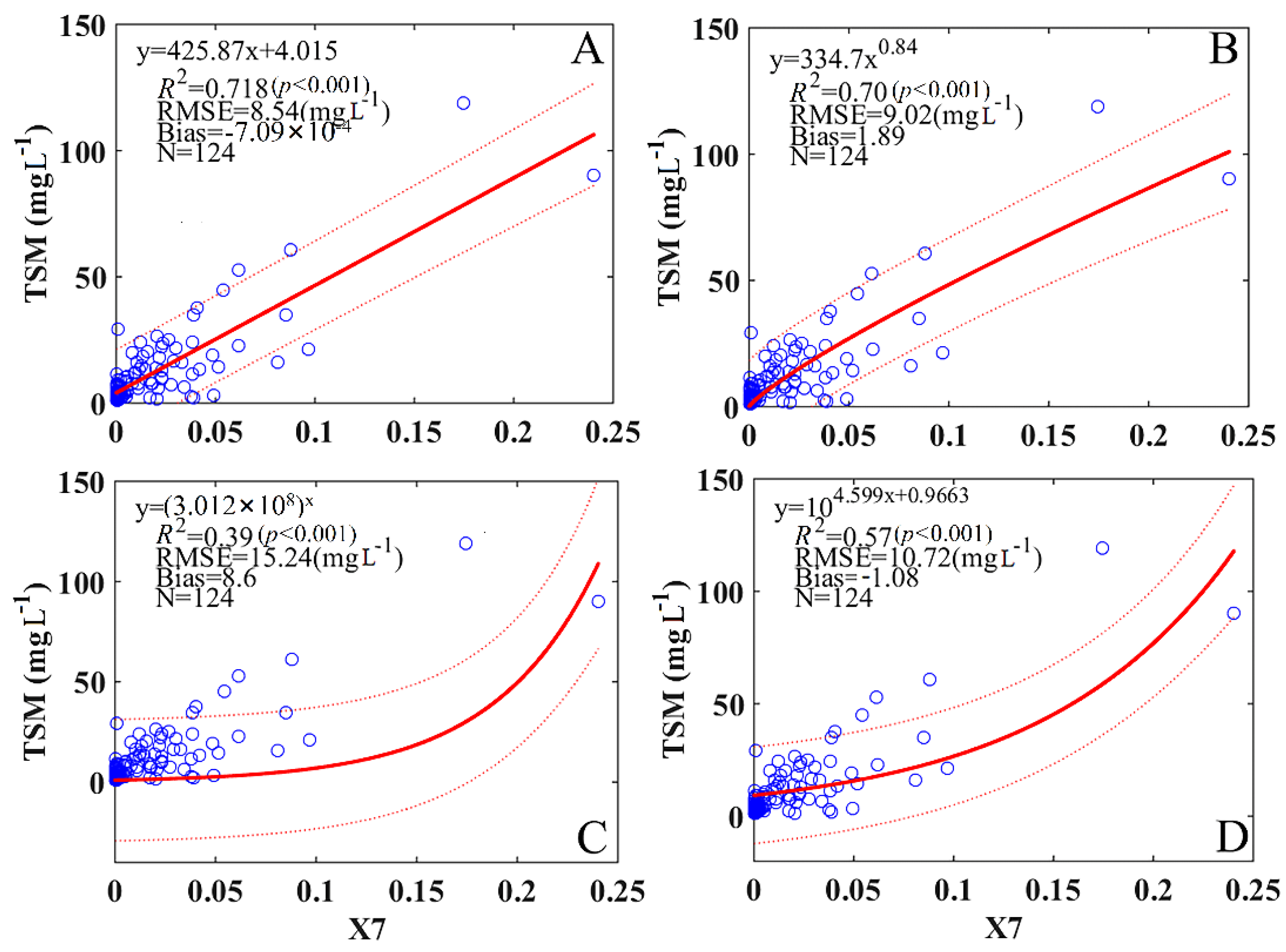
2.5.1. Estimation of TSM from
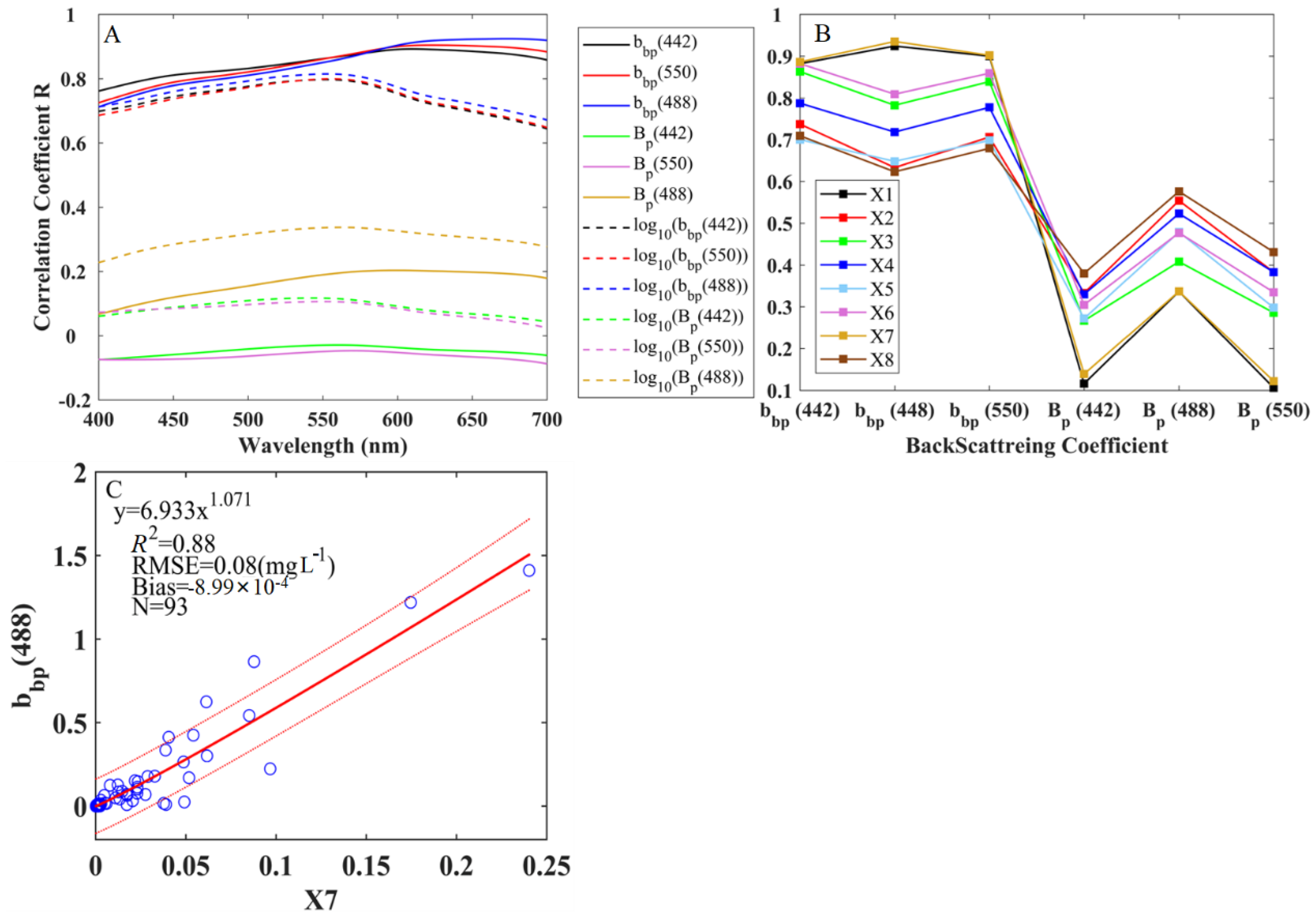
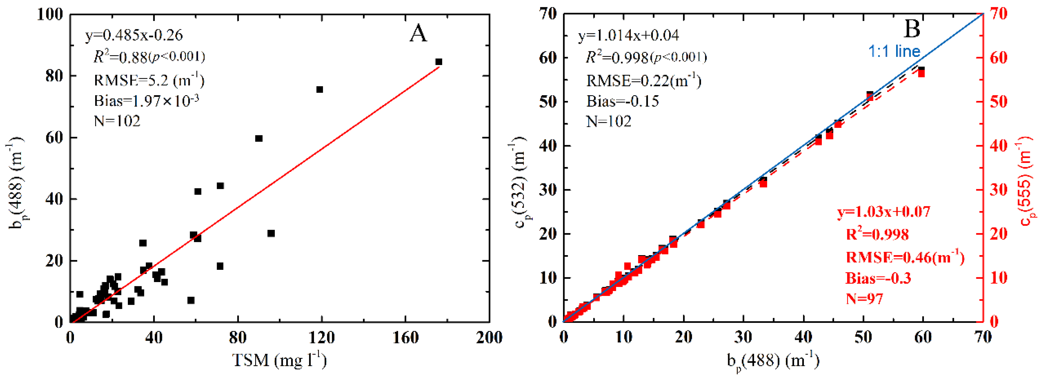
 R rs ( λ )

Estimation of TSM is a key step in retrieving the final target, np, by Rrs(λ). This study firstly analyzed the correlation between single Rrs(λ) and TSM in the spectral range of 400–700 nm, the results of which showed that the red bands were the most sensitive to TSM vis-à-vis the other bands (Figure 2). For instance, the correlation coefficients (R) showed high values (0.838 and 0.839) in the 660-nm and 680-nm bands of the GOCI image data, respectively. These findings also agree with those of previous studies [30,31]. These bands can be subsequently considered for use in establishing a TSM model.
Empirical methods are simple and easy to model and, more importantly, straight and efficient, particularly for local regions [32]. Thus, this study made use of single bands, band ratios, and band combinations to develop the TSM model. Specifically, eight band forms, as shown in Table 2, were tested. For each band form, the correlation with TSM was examined for all possible combinations from six GOCI Rrc(λ) bands, and the optimal band combinations with the highest R are given in Table 2. After comparing the correlations among these band forms, we determined X7, i.e., (Rrs(555) + Rrs(660))/(Rrs(555)/Rrs(660)), with the highest R of 0.847 among those band forms for establishing the TSM model. This method to find the optimal band form and optimal band combination was similar to that used in previous studies [33,34]. Several mathematical methods, including linear, power, exponential, and logarithmic functions, were used to model TSM, and their accuracies were then intercompared to obtain a good retrieval model. The obtained results showed that the simple linear model continued to perform best (Figure 3), and it was subsequently used to estimate TSM in our whole model framework.

2.5.2. Estimation of b bp and B p from R rs ( λ )

Estimation of the particulate backscattering coefficient, bbp(λ), is another important step. Similar to TSM estimation, this study firstly carried out a correlation analysis and then demonstrated that the X7 band combination form was the best indicator for the bbp(λ) estimation (Figure 4B). Note that the 488-nm channel was used to denote the parameter due to its better performance when compared to those of the other channels. After testing several different mathematical functions, we selected and established two strong relationships using the X7 form to model the bbp(488). As shown in Figure 4C, the fitted determination coefficient, R2, was 0.820 (p < 0.001), with relatively low predictive errors.

2.5.3. Derivation of the PSD Slope, j, from TSM

A close relationship between TSM and bp(488) could be established with relatively high fitting accuracy (Figure 5A), which was also consistent with that demonstrated in the He et al. [32] study. Meanwhile, very close relationships between bp(λ) and cp(λ) could also be found in our study area, as observed in previous studies [5,35,36,37]. As shown in Figure 5B, their relationships could be modeled well, with an extremely high R2 of 0.998 (p < 0.001). Such good relationships provide a stable basis for accurately deriving cp(λ) at different wavelengths from TSM. According to Equations (2) and (3), we obtained the parameter j, which was then used as an input of the model estimating np in this study.
As a summary, Figure 6 shows the main processes of our developed model in the current study to estimate the bulk refractive index np of particles by Rrs(λ). A Mie-theory-based relationship model was essentially adopted to derive np values from the so-called input parameters, namely, BP and j (Equation (1) by Twardowski et al. (2001) [2]), considering the fact that there are currently hardly any methods that can be used to directly measure the particle bulk refraction. Although some empirical relationships were used in the framework of our model development, the proposed np estimation model is a meaningful attempt to obtain satellite-derived np records.

2.6. Performance Metrics

To evaluate the models’ performances, this study utilized the root-mean-square error (RMSE), mean absolute error (MAE), mean relative error (MRE), determination coefficient (R2), and relative bias (Bias). These indicators can be calculated as follows:
RMSE = 1 N i = 1 N ( y i y i ) 2 ,
MAE = 1 N i = 1 N | y i y i | ,
MRE = 1 N i = 1 N | y i y i y i | ,
Bias = 1 N i = 1 N ( y i y i ) ,
where yi and yi’ are the measured and predictive values for the i-th sample, respectively, and N represents the total number of samples.

3. Results

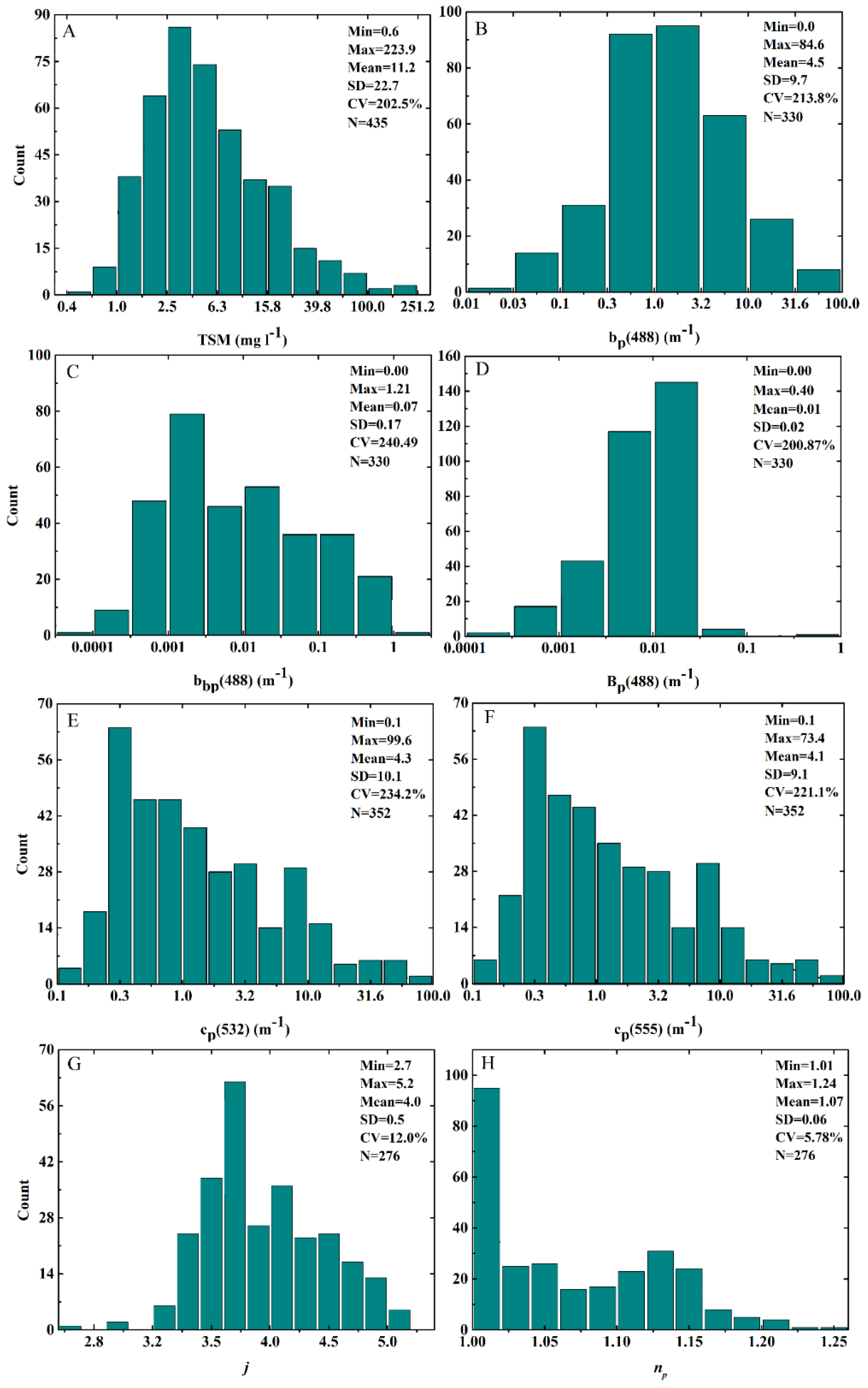
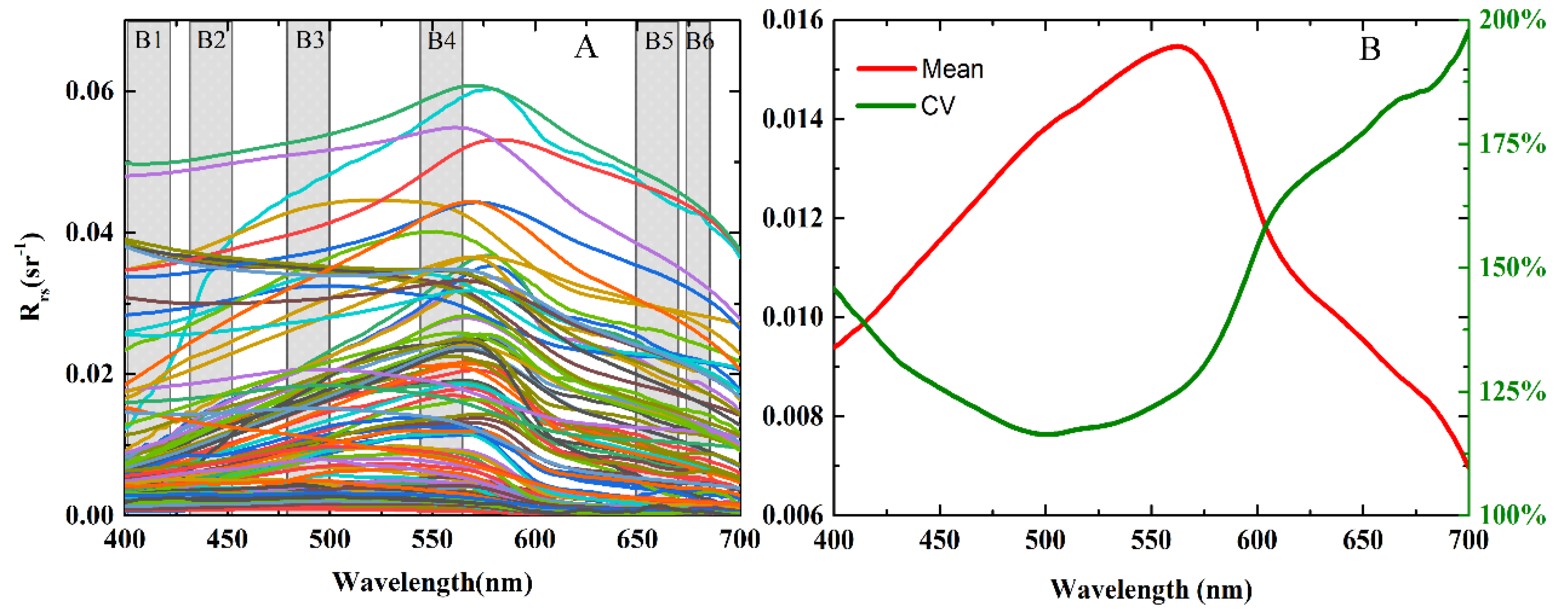
3.1. Water Bio-Optical Conditions

The bio-optical parameters in our investigated water regions showed very large dynamic ranges, which were collected from the four cruises (Figure 7). TSM varied from 0.6 to 223.9 mg∙L−1 and had a mean of 11.2 ± 22. 7 mg∙L−1. The large variation coefficient (CV)value (202.51%) indicates its large variation. The particulate backscattering coefficient at 488 nm, bbp (488), ranged between ~0 and 1.21 m−1, had a mean of 0.19 ± 0.17 m−1, and had a large CV (141.7%).
Correspondingly, the particulate scattering and beam attenuation coefficients, bp(488), cp(532), and cp(555), also showed wide variation ranges, as well as large CV values. The particulate backscattering ratio Bp(488), i.e., bbp/bp, changed from ~0 to 0.10 when the PSD slope, j, was observed to be in the range of 3.2–5.0. Note that a large span also appeared for the bulk refractive index of particles np. Meanwhile, the collected in situ Rrs(λ) showed large variations in terms of both magnitude and spectral shapes (Figure 8). These Rrs(λ) spectra had similar spectral properties to those seen in previous reports on coastal waters, for example, the studies of He et al. (2013) [32] and Sun et al. (2014) [36], which indicate typical optically complex turbid water conditions in the study area.

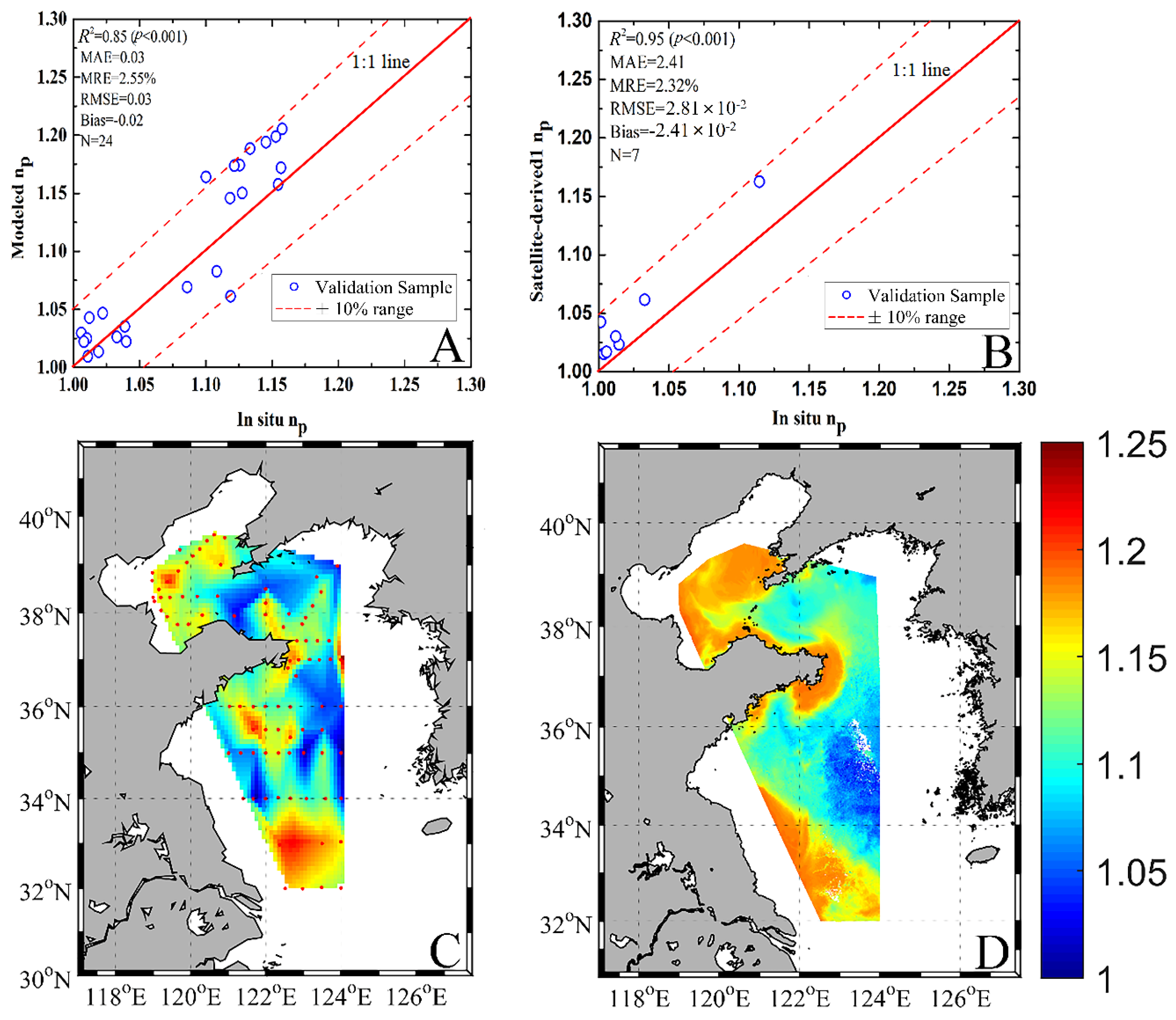
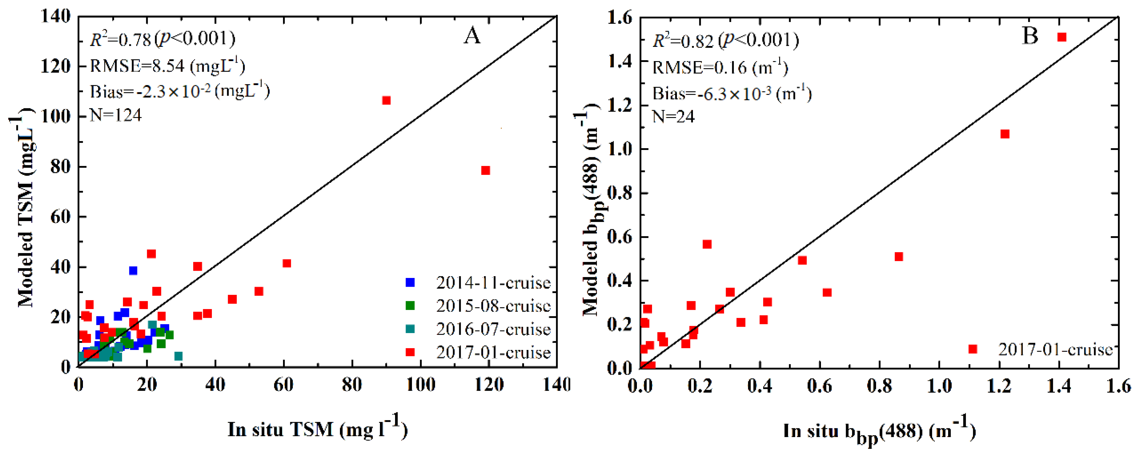
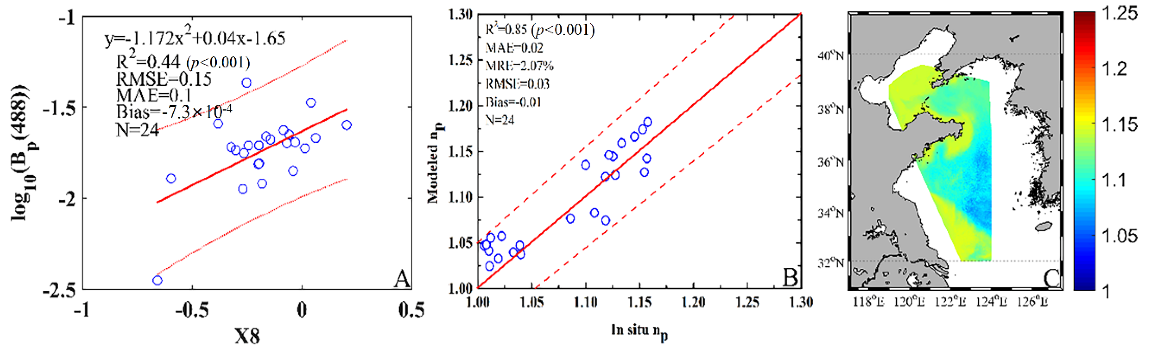
3.2. Validation of np Estimation Model

To evaluate the performance of the developed np model, we firstly used an independent validation dataset with 24 samples collected from the BS and YS in January 2017. As shown in Figure 9A, the modeled and in situ np values generally showed good clustering along the 1:1 line, with relatively low predictive errors. Most of the data points (approximately 84% percentage) were distributed within the ±5% range. On the other hand, this study carried out satellite synchronization verification. After matching GOCI satellite-derived Rrs data with in situ measurements using a set of strict constraints, a limited seven synchronous samples (±1 h) were obtained for use in comparisons between the in situ measured and satellite-derived np. Figure 9B shows the generally good agreement between them, with very low predictive errors (such as MRE = 2.32%), despite the modeled values being on the high side to some extent. This implies that the developed np model has the potential ability to produce accurate and acceptable results.
Additionally, we compared the spatial distributions of particle bulk refraction produced by in situ measurements and satellite derivation. Note that the satellite data used were from the specific monthly coverage concurrent with the cruise in January 2017. Figure 9C,D show the spatial patterns derived by in situ observations and satellite retrievals, respectively. Although there was no absolute real-time synchronization between the in situ measured and satellite-derived monthly np, the cruise sampling covered a period of nearly one month and was able to roughly provide an accurate reference. The generally similar spatial distributions of the in situ observations and satellite retrievals imply the accuracy of our developed np model.

3.3. Model Application to Satellite Data

We could produce hourly np products by applying the developed model into the hourly GOCI Rrs(λ) data. Those hourly products were then synthesized into daily, monthly, seasonally, and annually averaged products. As shown in Figure 10, the general distribution pattern for 2015 is available. High np values generally dominated nearshore waters, while low values were mainly distributed in the offshore waters. The whole BS region usually had relatively high refraction values of approximately >1.10, whereas most areas in the YS, except coastal regions, showed low values (roughly <1.05). Note that a large water region that includes Subei shoal and the Yangtze River estuary appeared to have very high refraction, which even exceeded 1.15 for some areas.
The seasonal and monthly variations in np in this study water areas were further generated as shown in Figure 11. On the whole, the np during the period from December 2014 to April 2015, as well as November 2015, appeared to have the most high-valued distribution throughout the entirety of the BS and YS regions, whereas relatively low values showed up between May and October 2015. In detail, in several particular water regions, including the Yellow River estuary, Yangtze River estuary, Subei shoal, and very nearshore areas, the np values remained almost static over time and were always high (>1.15) throughout the entire year. In most regions of the BS, the np values showed distinct seasonal variations, namely, high values in winter, early spring, and late autumn, whereas the values in summer were low. Similar temporal trends in np variation also appeared in the YS. However, the difference with that in the BS was that there existed generally lower np values in the YS for the same month.

4. Discussion

4.1. Advantages and Disadvantages of the np Model

The np model proposed in this study is a proof-of-concept remote sensing method for retrieving particulate refraction from GOCI satellite measurements in the study area. It is essentially dependent on the accurate retrievals of TSM and bbp, which are achieved by establishing stable empirical models. The variety of field measurements from the four cruises represents a prominent advantage in this study and provides a steady basis for developing the TSM and bbp empirical models. As shown in Figure 12, a leave-one-out cross-validation (LOO-CV) [38,39] was conducted to evaluate the performances of the TSM and bbp models. Briefly, we randomly selected one sample from the full dataset (sample number, n) that served for the validation of the model, while the remaining n − 1 samples were trained for model calibration. Based on the LOO-CV method, all samples were tried for one round, deriving relatively low and acceptable predictive errors. Thus, relatively accurate TSM and bbp retrievals, as well as their close relationships with bp and cp, provided a feasible route for achieving the estimation of np in the study areas. Another advantage lies in that there are more adequate remote sensing signals for model inputs when compared with the remote sensing method proposed by Nasiha et al. (2015) [5], which utilizes a single band reflectance (i.e., a green band at 551 nm) to derive the intermediate and target parameters. In addition to green band reflectance (555 nm), this study introduced red band reflectance, i.e., 660 nm, as another input, which assures more adequate valid remote sensing information that could potentially derive better outputs.
The developed np model may show limitations when it is applied to other coastal water areas. This is due to different optical properties that may vary with the change of study area because of the diversity and dynamics of in-water constituents [24,40,41,42,43,44]. Such local characteristics on water conditions generally determine region-specific empirical relationships between TSM (and bbp) and remote sensing reflectance and between bp (and cp) and TSM [16,17,45,46]. Nevertheless, these so-called limitations should not hinder the use of the proof-of-concept method proposed in this study for other regions. The same method with necessary local parameterizations can be employed to derive the particulate refraction using remote sensing data only if valid regional data can be obtained. However, in future, detailed investigations are still required to thoroughly assess the model’s applicability in various coastal water conditions. In addition, this study mainly focused on developing a method for estimating np from satellite data; thus, we used GOCI data as a case study. The applicability of the method to other satellite sensors is not clear, and further studies are also required to apply the similar method of this study to develop np estimation models specifically for MODIS, Visible infrared Imaging Radiometer (VIIRS), Landsat, etc., according to their band specifications, and then compare and cross-validate their performances.

4.2. Comparison with the Method Using a Straight Bp Empirical Model

The particulate backscattering ratio, Bp, is a straight input parameter to calculate np. In our developed np model, this parameter was obtained through the ratio by the modeled bbp and bp. However, we may still have another alternative, i.e., developing a Bp empirical model. By employing steps similar to those in Section 2.5.1 and Section 2.5.2, we developed an empirical relationship between Bp(488) and X8 that performed better than other functional models (see Figure 13A). By using the new method nested with the Bp empirical model, this study then obtained new np results, which showed roughly similar performance with that of the previous method (Figure 13B). However, note that the np spatial distribution derived by the new method was not very desirable, as there existed obvious overestimations for the offshore areas (Figure 13C). This was probably due to the fitted over-empirical relationship between Rrs and Bp of Yang et al., (2011) [47] because there is no physical linkage between them in theory, considering that Bp (= bbp/bp), especially bp therein, is essentially not retrievable from remote sensing owing to the fact that remote sensing covers no information on the forward scattering of suspended particles by Sun et al., (2016) [24]. By comparison, our proposed np retrieval method still showed superior performance in the study water areas.

4.3. Driving Factors of np Spatiotemporal Variation

By applying the developed np model to time-series GOCI satellite data, the np spatiotemporal variations in the study areas could be obtained, with the derived values spanning a range of 1.01–1.22 (Figure 10 and Figure 11). This variation in magnitude is generally consistent with that reported in previous studies [2,5,23,48,49]. In general, the np in the nearshore regions was higher than that offshore, noting that the nearshore regions showed relatively stable high values, whereas the offshore areas changed a lot during different seasons (or months). High-content mineral particles in the nearshore waters (e.g., the Yellow River estuary and Yangtze River estuary) induced by terrestrial discharge, sediment resuspension, and even shore erosion can explain the high np (1.12–1.18, see Figure 10) distribution there.
Regarding the offshore areas, the np values in the BS were higher than those in the YS. This is because the BS is prone to sediment resuspension under the action of wind waves due to its relatively shallow depths [50,51]. Song et al. (2014) [52] demonstrated that inorganic minerals and silts controlled the suspended particles in the BS. Therefore, those hard mineral and sediment particles may explain the high np values in the BS (except those nearshore regions), which were mainly in the range of 1.10–1.15 (Figure 10) [2,5,53]. Fortunately, the derived np distributions generally agree with the previous report [5]. By contrast, the YS waters (except those nearshore regions) are easily affected by algal particles, where diatoms and dinoflagellates are the main algal species [54,55,56]. Importantly, these algal particles generally show a relatively low bulk refraction (approximately 1.01–1.07) due to their high water content [57,58,59]. Therefore, the low refraction distribution in most regions of the YS (i.e., np < 1.07, see Figure 10) can be attributed to the dominance of organic algal particles.
From the perspective of the seasonal variations, the np showed the lowest distribution in summer for most areas of the BS and YS, whereas the highest distribution appeared in winter. The seasonal variations are probably related to water column mixing and stratification, as well as phytoplankton growth and extinction during different seasons [60,61]. Actually, the factors influencing the np distribution could be very complex, which may be linked with many marine physical and biogeochemical processes such as wind waves, river discharge, hydrodynamic conditions, water column mixing and stratification, sediment suspension, phytoplankton growth, and zooplankton grazing. In short, the precise understanding on the mechanisms influencing the np spatiotemporal variations remains challenging owing to the coupling influence of these multiple factors.

4.4. Implications for Marine Environmental Changes

The bulk refractive index of suspended particles (np) is a key parameter that reflects the intrinsic characteristics of suspended particles, is closely related to the particulate composition and size structures [2], and significantly affects the optical properties of suspended particles. Actually, different np distribution ranges are indicative of different types of suspended particles present in water bodies such as 1.01–1.09 mainly for organic algal particles, >1.15 for water regions dominated by inorganic particles and detritus, and 1.09–1.15 for complex and mixed particulates [2,3,48,49]. Satellite-derived np values in the study areas spanned a wide range (approximately 1.01–1.22), thus implying a large spatial heterogeneity. Three types of water regions can be generalized as (1) offshore oceanic water areas dominated by phytoplankton, (2) river plume and sediment-laden nearshore regions dominated by inorganic mineral particles, and (3) coastal regions controlled by organic and inorganic mixed materials. Although no in situ method exists for directly measuring the refractive index of suspended particles, the validation revealed the robustness of the currently proposed method to detect np for the study areas and further distinguish waters dominated by different types of suspended particles. In short, the spatiotemporal detection of np provides a new data record that enriches suspended particulate properties from space, and importantly improves understanding of the particulate biogeochemical properties and their role in exploring the changes of marine environments.

5. Conclusions

The current study proposed and validated a multiple-step hybrid remote sensing method to estimate np in the BS and YS from GOCI satellite measurements. This np estimation model depends on three crucial steps, namely, (1) the TSM and bbp retrievals, (2) establishing close relationships between bp and cp with TSM, and (3) utilizing the Twardowski et al. (2001) [2] model derived from Mie theory. The first two steps were calibrated and validated using a large quantity of in situ observed data from four cruises in the study area, whereas the third step was directly utilized, as it is widely recognized by the community. These steps jointly constructed our developed np estimation model in this study, which led to reliable performances with reasonable uncertainties (2.55% and 2.32% for MRE, validated using in situ observations with the leave-one-out cross-validation method and satellite-derived results, respectively) and spatial distribution patterns. By means of 2825 GOCI satellite images collected during one year from December 2014 to November 2015, this np estimation model documented np distribution patterns in the BS and YS at different temporal scales for the first time, such as monthly, seasonal, and annual scales. Although this method is possibly region-specific and may need more validation for its application to other water areas, the developed method here provides a proof-of-concept template for np remote sensing estimation in other coastal turbid water bodies.

Author Contributions

D.S. designed this study and the algorithm; Z.L. and S.W. contributed to the data analyses and drafted the manuscript; Z.Q. and Y.H. (Yu Huan) assisted with developing the research design and results interpretation; Z.M. and Y.H. (Yijun He) contributed to the interpretation of results and manuscript revision. All authors have read and agreed to the published version of the manuscript.

Funding

This research was funded by the National Key Research and Development Program of China (No. 2016YFC1400901), the National Natural Science Foundation of China (No. 41876203, 41576172), the Jiangsu Six Talent Summit Project (No. JY-084), the Qing Lan Project (No. R2019Q07), the Open Fund of State Key Laboratory of Satellite Ocean Environment Dynamics, Second Institute of Oceanography (No. QNHX1812), the Startup Foundation for Introducing Talent of NUIST (2019R058), the Science and Technology Innovation Project for Overseas Talents in Nanjing (R2019LZ05), and the CEReS Oversea Joint Research Program, Chiba University (No. CI19-103). This work was also sponsored by the NSFC Open Research Cruise (Cruise No. NORC2018-01), funded by the Shiptime Sharing Project of NSFC.

Acknowledgments

We acknowledge captains, officers, and crews of R/V Dongfanghong 2, Science 3, and Xiangyanghong 18 for providing excellent assistance during field sampling and measurements. We thank the Korea Ocean Satellite Center and NASA for providing satellite data.

Conflicts of Interest

The authors declare no conflicts of interest.

References

  1. Stramski, D.; Bricaud, A.; Morel, A. Modeling the inherent optical properties of the ocean based on the detailed composition of the planktonic community. Appl. Opt. 2001, 40, 2929. [Google Scholar] [CrossRef] [PubMed]
  2. Twardowski, M.S.; Emmanuel, B.; Macdonald, J.B.; Scott, P.W.; Barnard, A.H.; Zaneveld, J.R.V. A model for estimating bulk refractive index from the optical backscattering ratio and the implications for understanding particle composition in case I and case II waters. J. Geophys. Res. Atmos. 2001, 106, 14129–14142. [Google Scholar] [CrossRef] [Green Version]
  3. Woźniak, S.B.; Stramski, D. Modeling the optical properties of mineral particles suspended in seawater and their influence on ocean reflectance and chlorophyll estimation from remote sensing algorithms. Appl. Opt. 2004, 43, 3489–3503. [Google Scholar] [CrossRef] [PubMed]
  4. Nasiha, H.J.; Shanmugam, P.; Hariharasudhan, V.G. A new inversion model to estimate bulk refractive index of particles in coastal oceanic waters: Implications for remote sensing. IEEE J. Sel. Top. Appl. Earth Obs. Remote Sens. 2014, 7, 3069–3083. [Google Scholar] [CrossRef]
  5. Nasiha, H.J.; Shanmugam, P. Estimating the bulk refractive index and related particulate properties of natural waters from remote-sensing data. IEEE J. Sel. Top. Appl. Earth Obs. Remote Sens. 2015, 8, 5324–5335. [Google Scholar] [CrossRef]
  6. Pak, H.; Ronald, J.; Zaneveld, V. Method for the determination of the index of refraction of particles suspended in the ocean. Domest. Anim. Endocrinol. 2010, 38, 115–125. [Google Scholar]
  7. Yentsch, C.S. A note on the fluorescence characteristics of particles that pass through glass-fiber filters. Limnol. Oceanogr. 1983, 28, 597–599. [Google Scholar] [CrossRef]
  8. Agrawal, Y.C.; Pottsmith, H.C. Instruments for particle size and settling velocity observations in sediment transport. Mar. Geol. 2000, 168, 89–114. [Google Scholar] [CrossRef]
  9. Jonasz, M.; Fournier, G.R. Light Scattering by Particles in Water; ELSEVIER: Amsterdam, The Netherlands, 2017; pp. 611–681. [Google Scholar]
  10. Gitelson, A.A.; Dall’Olmo, G.; Moses, W.; Rundquist, D.C.; Barrow, T.; Fisher, T.R.; Gurlin, D.; Holz, J. A simple semi-analytical model for remote estimation of chlorophyll-a in turbid waters: Validation. Remote Sens. Environ. 2008, 112, 3582–3593. [Google Scholar] [CrossRef]
  11. Hu, C.; Lee, Z.; Franz, B. Chlorophyll aalgorithms for oligotrophic oceans: A novel approach based on three-band reflectance difference. J. Geophys. Res. Ocean. 2012, 117, C01011. [Google Scholar] [CrossRef] [Green Version]
  12. O’Reilly, J.E.; Maritorena, S.; Siegel, D.A.; O’Brien, M.C.; Toole, D.; Mitchell, B.G.; Kahru, M.; Chavez, F.P.; Strutton, P.; Cota, G.F. Ocean color chlorophyll a algorithms for seawifs, oc2, and oc4: Version 4. SeaWiFS Postlaunch Calibration Valid. Anal. 2000, 3, 9–23. [Google Scholar]
  13. Tilstone, G.H.; Angel-Benavides, I.M.; Pradhan, Y.; Shutler, J.D.; Groom, S.; Sathyendranath, S. An assessment of chlorophyll-a algorithms available for seawifs in coastal and open areas of the bay of bengal and arabian sea. Remote Sens. Environ. 2011, 115, 2277–2291. [Google Scholar] [CrossRef]
  14. Werdell, P.J.; Bailey, S.W.; Franz, B.A.; Harding, L.W., Jr.; Feldman, G.C.; McClain, C.R. Regional and seasonal variability of chlorophyll-a in chesapeake bay as observed by seawifs and MODIS-Aqua. Remote Sens. Environ. 2009, 113, 1319–1330. [Google Scholar] [CrossRef]
  15. Kishino, M.; Tanaka, A.; Ishizaka, J. Retrieval of chlorophyll a, suspended solids, and colored dissolved organic matter in tokyo bay using aster data. Remote Sens. Environ. 2005, 99, 66–74. [Google Scholar] [CrossRef]
  16. Nechad, B.; Ruddick, K.G.; Park, Y. Calibration and validation of a generic multisensor algorithm for mapping of total suspended matter in turbid waters. Remote Sens. Environ. 2010, 114, 854–866. [Google Scholar] [CrossRef]
  17. Ondrusek, M.; Stengel, E.; Kinkade, C.S.; Vogel, R.L.; Keegstra, P.; Hunter, C.; Kim, C. The development of a new optical total suspended matter algorithm for the chesapeake bay. Remote Sens. Environ. 2012, 119, 243–254. [Google Scholar] [CrossRef] [Green Version]
  18. Dogliotti, A.I.; Ruddick, K.G.; Nechad, B.; Doxaran, D.; Knaeps, E. A single algorithm to retrieve turbidity from remotely-sensed data in all coastal and estuarine waters. Remote Sens. Environ. 2015, 156, 157–168. [Google Scholar] [CrossRef] [Green Version]
  19. Qiu, Z.; Zheng, L.; Zhou, Y.; Sun, D.; Wang, S.; Wu, W. Innovative goci algorithm to derive turbidity in highly turbid waters: A case study in the zhejiang coastal area. Opt. Express 2015, 23, A1179. [Google Scholar] [CrossRef]
  20. Chen, J.; He, X.; Zhou, B.; Pan, D. Deriving colored dissolved organic matter absorption coefficient from ocean color with a neural quasi-analytical algorithm. J. Geophys. Res. Ocean. 2017, 122, 8543–8556. [Google Scholar] [CrossRef]
  21. Mannino, A.; Russ, M.E.; Hooker, S.B. Algorithm development and validation for satellite-derived distributions of doc and cdom in the U.S. Middle atlantic bight. J. Geophys. Res. Ocean. 2008, 113. [Google Scholar] [CrossRef]
  22. Zhu, W.; Yu, Q.; Tian, Y.Q.; Becker, B.L.; Zheng, T.; Carrick, H.J. An assessment of remote sensing algorithms for colored dissolved organic matter in complex freshwater environments. Remote Sens. Environ. 2014, 140, 766–778. [Google Scholar] [CrossRef]
  23. Suresh, T.; Desa, E.; Mascaranahas, A.; Matondkar, S.G.P.; Naik, P.; Nayak, S.R. An empirical method to estimate bulk particulate refractive index for ocean satellite applications. In Remote Sensing of the Marine Environment; International Society for Optics and Photonics: Bellingham WA, USA, 2006; Volume 6406, p. 64060B. [Google Scholar]
  24. Sun, D.; Qiu, Z.; Hu, C.; Wang, S.; Wang, L.; Zheng, L.; Peng, T.; He, Y. A hybrid method to estimate suspended particle sizes from satellite measurements over Bohai Sea and Yellow Sea. J. Geophys. Res. Ocean. 2016, 121, 6742–6761. [Google Scholar] [CrossRef]
  25. Sun, D.; Huan, Y.; Qiu, Z.; Hu, C.; Wang, S.; He, Y. Remote sensing estimation of phytoplankton size classes from GOCI satellite measurements in Bohai Sea and Yellow Sea. J. Geophys. Res. Ocean. 2017, 122, 8309–8325. [Google Scholar] [CrossRef]
  26. Voss, K.J. A spectral model of the beam attenuation coefficient in the ocean and coastal areas. Limnol. Oceanogr. 1992, 37, 501. [Google Scholar] [CrossRef] [Green Version]
  27. Roesler, C.S.; Boss, E. Spectral beam attenuation coefficient retrieved from ocean color inversion. Geophys. Res. Lett. 2003, 30. [Google Scholar] [CrossRef] [Green Version]
  28. Boss, E.; Pegau, W.S.; Gardner, W.D.; Zaneveld, J.R.V.; Barnard, A.H.; Twardowski, M.S.; Chang, G.C.; Dickey, T.D. Spectral particulate attenuation and particle size distribution in the bottom boundary layer of a continental shelf. J. Geophys. Res. Ocean. 2001, 106, 9509–9516. [Google Scholar] [CrossRef] [Green Version]
  29. Wang, M.; Gordon, H.R. A simple, moderately accurate, atmospheric correction algorithm for SeaWiFS. Remote Sens. Environ. 1994, 50, 231–239. [Google Scholar] [CrossRef]
  30. Goodin, D.G.; Harrington, J.A., Jr.; Nellis, M.D.; Rundquist, D.C. Mapping reservoir turbidity patterns using spot-hrv data. Geocarto Int. 1996, 11, 71–78. [Google Scholar] [CrossRef]
  31. Ouillon, S.; Douillet, P.; Petrenko, A.; Neveux, J.; Dupouy, C.; Froidefond, J.M.; Andréfouët, S.; Muñoz-Caravaca, A. Optical algorithms at satellite wavelengths for total suspended matter in tropical coastal waters. Sensors 2008, 8, 4165–4185. [Google Scholar] [CrossRef]
  32. He, X.; Bai, Y.; Pan, D.; Huang, N.; Dong, X.; Chen, J.; Chen, C.T.A.; Cui, Q. Using geostationary satellite ocean color data to map the diurnal dynamics of suspended particulate matter in coastal waters. Remote Sens. Environ. 2013, 133, 225–239. [Google Scholar] [CrossRef]
  33. Wang, S.; Huan, Y.; Qiu, Z.; Sun, D.; Zhang, H.; Zheng, L.; Xiao, C. Remote Sensing of Particle Cross-Sectional Area in the Bohai Sea and Yellow Sea: Algorithm Development and Application Implications. Remote Sens. 2016, 8, 841. [Google Scholar] [CrossRef] [Green Version]
  34. Niroumand-Jadidi, M.; Bovolo, F.; Bruuzone, L. Novel Spectra-Derived Features for Empirical Retrieval of Water Quality Parameters: Demonstrations for OLI, MSI, and OLCI Sensors. IEEE Trans. Geosci. Remote Sens. 2019, 57, 10285–10300. [Google Scholar] [CrossRef]
  35. Kirk, J. Monte carlo study of the nature of the underwater light field in, and the relationships between optical properties of, turbid yellow waters. Mar. Freshw. Res. 1981, 32, 517–532. [Google Scholar] [CrossRef]
  36. Sun, D.; Hu, C.; Qiu, Z.; Cannizzaro, J.P.; Barnes, B.B. Influence of a red band-based water classification approach on chlorophyll algorithms for optically complex estuaries. Remote Sens. Environ. 2014, 155, 289–302. [Google Scholar] [CrossRef]
  37. Davies-Colley, R.J.; Nagels, J.W. Predicting light penetration into river waters. J. Geophys. Res. Biogeosci. 2015, 113, 375–402. [Google Scholar] [CrossRef]
  38. Kearns, M.; Ron, D. Algorithmic stability and sanity-check bounds for leave-one-out cross-validation. Neural Comput. 1997, 11, 1427–1453. [Google Scholar] [CrossRef]
  39. Cawley, G.C. Leave-one-out cross-validation based model selection criteria for weighted ls-svms. In Proceedings of the 2006 IEEE International Joint Conference on Neural Networks, Vancouver, BC, Canada, 16–21 July 2006. [Google Scholar]
  40. Babin, M.; Morel, A.; Fournier-Sicre, V.; Fell, F.; Stramski, D. Light scattering properties of marine particles in coastal and open ocean waters as related to the particle mass concentration. Limnol. Oceanogr. 2003, 48, 843–859. [Google Scholar] [CrossRef]
  41. Loisel, H.; Mériaux, X.; Berthon, J.F.; Poteau, A. Investigation of the optical backscattering to scattering ratio of marine particles in relation to their biogeochemical composition in the eastern english channel and southern north sea. Limnol. Oceanogr. 2007, 52, 739–752. [Google Scholar] [CrossRef]
  42. Whitmire, A.L.; Boss, E.; Cowles, T.J.; Pegau, W.S. Spectral variability of the particulate backscattering ratio. Opt. Express 2007, 15, 7019–7031. [Google Scholar] [CrossRef] [Green Version]
  43. Snyder, W.A.; Arnone, R.A.; Davis, C.O.; Goode, W.; Gould, R.W.; Ladner, S.; Lamela, G.; Rhea, W.J.; Stavn, R.; Sydor, M. Optical scattering and backscattering by organic and inorganic particulates in U.S. Coastal waters. Appl. Opt. 2008, 47, 666. [Google Scholar] [CrossRef] [Green Version]
  44. Zhang, M.; Tang, J.; Song, Q.; Dong, Q. Backscattering ratio variation and its implications for studying particle composition: A case study in yellow and east china seas. J. Geophys. Res. Ocean. 2010, 115. [Google Scholar] [CrossRef]
  45. Doña, C.; Sánchez, J.M.; Caselles, V.; Domínguez, J.A.; Camacho, A. Empirical relationships for monitoring water quality of lakes and reservoirs through multispectral images. IEEE J. Sel. Top. Appl. Earth Obs. Remote Sens. 2014, 7, 1632–1641. [Google Scholar] [CrossRef]
  46. Wang, X.; Fu, L.; He, C. Applying support vector regression to water quality modelling by remote sensing data. Int. J. Remote Sens. 2011, 32, 8615–8627. [Google Scholar] [CrossRef]
  47. Yang, W.; Matsushita, B.; Chen, J.; Fukushima, T. Estimating constituent concentrations in case ii waters from meris satellite data by semi-analytical model optimizing and look-up tables. Remote Sens. Environ. 2011, 115, 1247–1259. [Google Scholar] [CrossRef] [Green Version]
  48. Boss, E.; Pegau, W.S.; Lee, M.; Twardowski, M.; Shybanov, E.; Korotaev, G.; Baratange, F. Particulate backscattering ratio at leo 15 and its use to study particle composition and distribution. J. Geophys. Res. Ocean. 2004, 109. [Google Scholar] [CrossRef] [Green Version]
  49. Sullivan, J.M.; Twardowski, M.S.; Donaghay, P.L.; Freeman, S.A. Use of optical scattering to discriminate particle types in coastal waters. Appl. Opt. 2005, 44, 1667–1680. [Google Scholar] [CrossRef]
  50. Cui, T.; Zhang, J.; Ma, Y.; Zhao, W.; Sun, L. The study on the distribution of suspended particulate matter in the bohai sea by remote sensing. Acta Oceanol. Sin. 2009, 31, 10–18. [Google Scholar]
  51. Cui, T.W.; Jie, Z.; Groom, S.; Ling, S.; Smyth, T.; Sathyendranath, S. Validation of meris ocean-color products in the bohai sea: A case study for turbid coastal waters. Remote Sens. Environ. 2010, 114, 2326–2336. [Google Scholar] [CrossRef]
  52. Song, Q.; Zhang, J.; Cui, T.; Bao, Y. Remote sensing retrieval of inorganic suspended particle size in the bohai sea. Cont. Shelf Res. 2014, 73, 64–71. [Google Scholar]
  53. Lide, D.R. (Ed.) Physical and optical properties of minerals. In CRC Handbook of Chemistry and Physics, 77th ed.; CRC Press: Boca Raton, FL, USA, 1997; pp. 4.130–4.136. [Google Scholar]
  54. Hu, C.; Li, D.; Chen, C.; Ge, J.; Muller-Karger, F.E.; Liu, J.; Yu, F.; He, M.X. On the recurrent ulva prolifera blooms in the yellow sea and east china sea. J. Geophys. Res. Ocean. 2010, 115, C05017. [Google Scholar] [CrossRef] [Green Version]
  55. Guo, S.J.; Sun, J.; Zhang, H.; Zai, W.D. Phytoplankton communities in the northern yellow sea in autumn 2011. J. Tianjin Univ. Sci. Technol. 2013, 28, 22–29. [Google Scholar]
  56. Nie, J.J.; Liu, Y.J.; Feng, Z.Q.; Yang, Q.; Liu, G.Z.; Fan, J.F. Phytoplankton community in the north yellow sea in spring and yearly variation. Mar. Environ. Sci. 2014, 33, 182–207. [Google Scholar]
  57. Carder, K.L.; Tomlinson, R.D.; Beardsley, G.F. A technique for the estimation of indices of refraction of marine phytoplankters. Limnol. Oceanogr. 1972, 17, 833–839. [Google Scholar] [CrossRef]
  58. Stramski, D.; Morel, A.; Bricaud, A. Modeling the light attenuation and scattering by spherical phytoplanktonic cells: A retrieval of the bulk refractive index. Appl. Opt. 1988, 27, 3954. [Google Scholar] [CrossRef] [PubMed]
  59. Aas, E. Refractive index of phytoplankton derived from its metabolite composition. J. Plankton Res. 1996, 18, 2223–2249. [Google Scholar] [CrossRef] [Green Version]
  60. Chen, C.T.A. Chemical and physical fronts in the bohai, yellow and east china seas. J. Mar. Syst. 2009, 78, 394–410. [Google Scholar] [CrossRef]
  61. Xu, Y.; Siswanto, E.; Wang, S. Relationships of interannual variability in sst and phytoplankton blooms with giantjellyfish (nemopilema nomurai) outbreaks in the yellow sea and east china sea. J. Oceanogr. 2013, 69, 511–526. [Google Scholar] [CrossRef] [Green Version]
Figure 1. Bathymetry map of the study areas (Bohai Sea and Yellow Sea) overlaid with the stations collected from the four cruises in November 2014, August 2015, July 2016, and January 2017. The red rectangles refer to those stations with remote sensing reflectance, Rrs(λ), data, and different colors indicate different water depths.
Applsci 10 00023 g001
Figure 2. Correlation coefficient spectra between total suspended matter (TSM) and Rrs(λ) in the range of 400–700 nm.
Applsci 10 00023 g002
Figure 3. Scatter plots of X7 and TSM using different mathematical functions ((A) linear, (B) power, (C) exponential, and (D) logarithmic functions), overlaid by model accuracies and function expressions. X7 refers to (Rrs(555) + Rrs(660))/(Rrs(555)/Rrs(660)). The solid red lines are the fitted function curves, and the dotted red lines are the 95% confidence bounds.
Applsci 10 00023 g003
Figure 4. (A) Correlation coefficient spectra between Rrs(λ) and bbp(λ) and log10(bbp(λ)) in the range of 400–700 nm; (B) correlation coefficients between bbp(λ) and eight band combination forms (X1 to X8), which are the same as those in Figure 4. (C) Scatter plots of X7 (i.e., (Rrs(555) + Rrs(660))/(Rrs(555)/Rrs(660))) and bbp(488) using a power function; the solid red lines are the fitted function curves, and the dotted red lines are the 95% confidence bounds.
Applsci 10 00023 g004
Figure 5. Relationships (A) between TSM and bp(488), and (B) between bp(488) and cp(532) and cp(555), which were observed in January 2017. These close relationships all show a very high confidence level, with p < 0.001.
Applsci 10 00023 g005
Figure 6. Flow diagram of our developed np estimation model that shows the steps of deriving np from Rrs(λ). The shown different colors in the legend refer to different processes, namely, inputs, calculations, models, and outputs.
Applsci 10 00023 g006
Figure 7. Frequency distributions of (A) TSM, (B) bp(488), (C) bp(488), (D) Bp(488), (E) cp(532), (F) cp(555), (G) particle size distribution (PSD) slope, j, and (H) np. The black lines represent log-normal distribution fitting curves.
Applsci 10 00023 g007
Figure 8. (A) In situ Rrs(λ) observed from the four cruises in the present study, overlaid by GOCI (Geostationary Ocean Color Imager) six channels (gray bars); (B) mean Rrs(λ) spectrum and variation coefficient (CV) spectral curve.
Applsci 10 00023 g008
Figure 9. Scatter plots show the in situ np values versus those values derived from the developed model by means of in situ observed Rrs data (A) and GOCI satellite-derived np values (B). The solid red lines refer to the 1:1 lines, and the dotted lines indicate the ±5% ranges of deviation relative to the central line. The np spatial patterns derived from the in situ measurements (C) and the GOCI satellite retrievals (D) in January 2017 were also compared.
Applsci 10 00023 g009
Figure 10. Annual distribution pattern of np derived by our developed model, based on GOCI data of the whole year of 2015.
Applsci 10 00023 g010
Figure 11. Seasonal distribution patterns of the np estimated by our developed model using GOCI satellite observations during 2015 using the np model developed in this study.
Applsci 10 00023 g011
Figure 12. Comparison between in situ and modeled (A) TSM and (B) b bp ( 488 ) for the leave-one-out cross-validation. The colors indicate different cruise datasets.
Applsci 10 00023 g012
Figure 13. (A) Scatter plots of X8 (i.e., −log10(Rrs(680))) and Bp(488) using a quadratic function. This function was found to perform best among the other functions. The solid red lines are the fitted function curves, and the dotted red lines are the 95% confidence bounds. (B) Scatter plots of the in situ np values versus those predicted from the new method with the developed Bp model. (C) Spatial distribution of the np derived from GOCI satellite observations in January 2017 using this new method.
Applsci 10 00023 g013
Table 1. Description of in situ observed datasets collected during four cruise surveys in the study area. TSM—total suspended matter.
Cruise DateMeasured ParametersSample Numbers
7 November 2014–23 November 2014Rrs(λ) (sr−1)27
TSM (mg∙L−1)108
17 August 2015–5 September 2015Rrs(λ) (sr−1)37
TSM (mg∙L−1)101
29 June 2016–14 July 2016Rrs(λ) (sr−1)58
TSM (mg∙L−1)123
29 December 2016–13 January 2017Rrs(λ) (sr−1)24
TSM (mg∙L−1)103
bbp (m−1)102
bp (m−1)102
cp (m−1)103
Table 2. Correlations between TSM and band form X derived from GOCI (Geostationary Ocean Color Imager) six bands. X1 to X8 indicate eight band forms, respectively; R is the correlation coefficient.
XDetailed Band FormOptimal Band CombinationR
X1Rrs(λ1)λ1 = 680 nm0.839
X2log10(Rrs(λ1))λ1 = 680 nm0.588
X3Rrs1) − Rrs(λ2)λ1 = 660 nm, λ2 = 680 nm0.725
X4 R rs ( λ 1 ) R rs ( λ 2 ) λ1 = 660 nm, λ2 = 555 nm0.606
X5 log 10 R rs ( λ 1 ) log 10 R rs ( λ 2 ) λ1 = 490 nm, λ2 = 660 nm0.581
X6 R rs λ 1 R rs ( λ 2 ) R rs λ 1 / R rs ( λ 2 ) λ1 = 660 nm, λ2 = 680 nm0.739
X7 R rs λ 1 + R rs ( λ 2 ) R rs ( λ 1 ) / R rs ( λ 2 ) λ1 = 555 nm, λ2 = 660 nm0.847
X8 R rs λ 1 R rs ( λ 2 ) R rs ( λ 1 ) + R rs ( λ 2 ) λ1 = 660 nm, λ2 = 555 nm0.555

