Antiderivative Antialiasing for Stateful Systems ^†

Abstract

Nonlinear systems, such as guitar distortion effects, play an important role in musical signal processing. One major problem encountered in digital nonlinear systems is aliasing distortion. Consequently, various aliasing reduction methods have been proposed in the literature. One of these is based on using the antiderivative of the nonlinearity and has proven effective, but is limited to memoryless systems. In this work, it is extended to a class of stateful systems which includes but is not limited to systems with a single one-port nonlinearity. Two examples from the realm of virtual analog modeling show its applicability to and effectiveness for commonly encountered guitar distortion effect circuits.

1. Introduction

Nonlinear systems play an important role in musical signal processing. In particular, there are many effects categorized as overdrive, distortion, or fuzz, whose primary objective is to introduce harmonic distortion to enrich the signal. Usually, the nonlinear behavior is combined with (linear) filtering to spectrally shape the output signal or to make the amount of introduced distortion frequency-dependent. While many of these systems were originally designed in the analog domain, naturally, there is interest in deriving digital models for them, e.g., [1,2,3,4].

One major problem encountered in digital nonlinear systems, whether designed from scratch or derived by virtual analog modeling is aliasing distortion. Once the additional harmonics introduced by the nonlinearity exceed the Nyquist limit at half the sampling frequency, they get folded back to lower frequencies, just as if the corresponding analog signal had been sampled without appropriate band-limiting. Contrary to the desired harmonic distortion, aliasing distortion is usually perceived as unpleasant. Therefore, methods to suppress or reduce aliasing distortion are needed.

The conceptually simplest aliasing reduction method is oversampling. However, if the harmonics decay slowly with frequency, the oversampling factor has to be high, making the approach unattractive due to the rising computational demand. Consequently, various alternatives have been proposed, e.g., [5,6,7,8,9,10,11]. These methods, however, usually come with certain limitations, most commonly the restriction to memoryless systems. In this work, an extension of [10] is presented that loosens the restriction from memoryless systems to a certain class of stateful systems.

This article is an extension of our previous conference paper [12]. The main differences are the generalization of the method to the case of multiple parallel nonlinear functions and an added discussion of nonlinearities with vector-valued input.

2. Antiderivative-Based Aliasing Reduction for Memoryless Nonlinear Systems

As the proposed method builds upon the approach from [10], we shall briefly summarize the latter. Conceptually, the digital signal is converted to a continuous-time signal using linear interpolation between consecutive samples, the nonlinearity is applied, and the result is lowpass-filtered by integrating over one sampling interval before sampling again to obtain the digital output signal. Thus, the nonlinear system

$$y\left(n\right)=f\left(u\left(n\right)\right),$$

(1)

where $f\left(u\right)$ denotes the nonlinear function, mapping input sample $u\left(n\right)$ to output sample $y\left(n\right)$, is transformed into

$$y\left(n\right)={\int }_0^{1}f\left({\overline{u}}_n\left(\tau \right)\right)d\tau \mathrm{with}{\overline{u}}_n\left(\tau \right)=(1-\tau )u(n-1)+\tau u\left(n\right).$$

(2)

Only rarely, the integral will have a closed solution and numerical integration at run time is unattractive considering the computational load. However, by switching the integration variable, we obtain

$$y\left(n\right)=\frac{1}{u\left(n\right)-u(n-1)}{\int }_{u(n-1)}^{u\left(n\right)}f\left(\overline{u}\right)d\overline{u},$$

(3)

where we may apply the fundamental theorem of calculus and by further special-casing $u\left(n\right)\approx u(n-1)$ to avoid numerical issues, we finally arrive at

$$y\left(n\right)=\tilde{f}\left(u\left(n\right),u(n-1)\right)=\left\{\begin{array}{cc}\frac{F\left(u\right(n\left)\right)-F\left(u\right(n-1\left)\right)}{u\left(n\right)-u(n-1)}\hfill & \mathrm{if}u\left(n\right)\approx u(n-1)\hfill \\ f\left(\frac{1}{2}u\left(n\right)+\frac{1}{2}u(n-1)\right)\hfill & \mathrm{if}u\left(n\right)\approx u(n-1)\hfill \end{array}\right.$$

(4)

where $F\left(u\right)=\int f\left(u\right)du$ is the antiderivative of $f\left(u\right)$. Again, the antiderivative may not have a closed solution, but being a function in one variable, it may be pre-computed and stored in a lookup table.

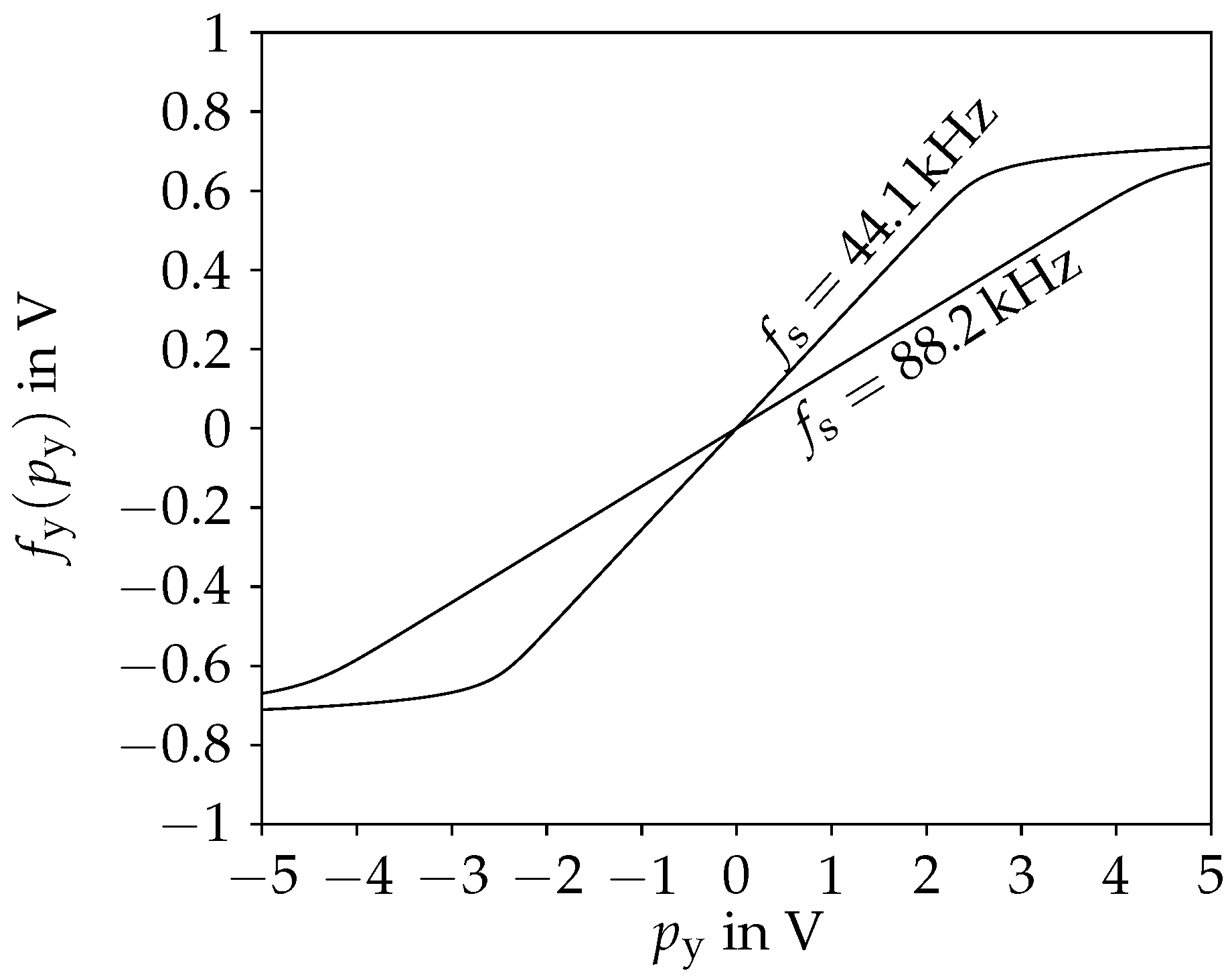
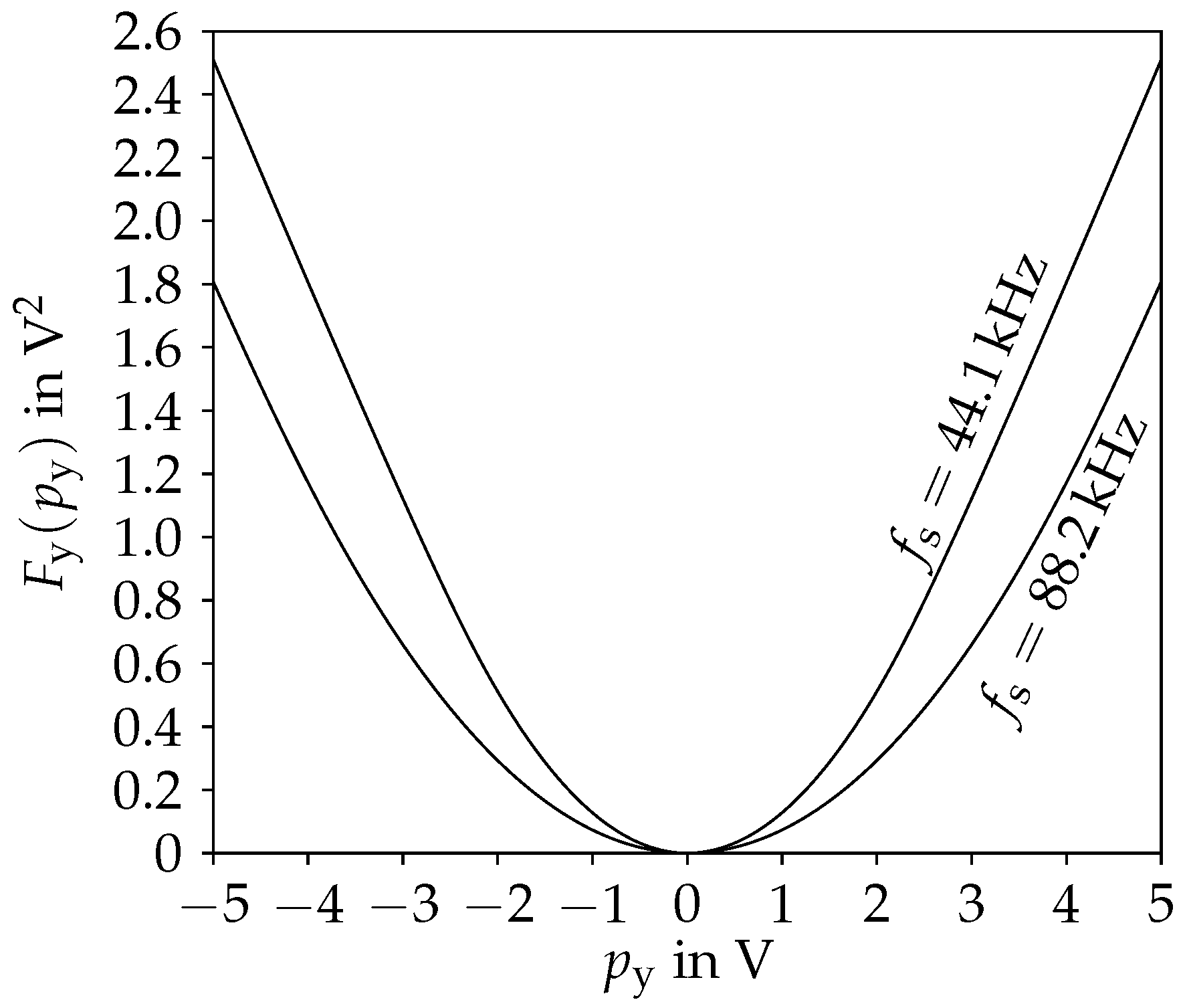
In addition to reducing aliasing artifacts, the approach introduces a half-sample delay and attenuates signal components not only above the Nyquist limit, but also at high frequencies below it, i.e., it acts as a low-pass filter in the audio band. This can be readily seen when using the identity function $f\left(u\right)=u$ instead of a true nonlinearity. In that case, straightforward calculation yields

$$y\left(n\right)=\frac{1}{2}u\left(n\right)+\frac{1}{2}u(n-1),$$

(5)

which is a first-order finite impulse response low-pass filter with a group delay of half a sample. The low-pass effect can be countered by a modest amount of oversampling (e.g., by a factor of two) and the delay usually is of no concern.

The Higher-Dimensional Case

Before turning to stateful systems, we shall briefly discuss how to lift the restriction to systems with one scalar input $u\left(n\right)$ and one scalar output $y\left(n\right)$ quietly assumed so far. To keep the notation concise, we collect the inputs $u_1\left(n\right),u_2\left(n\right),\dots ,u_{K_{\mathrm{u}}}\left(n\right)$ of a system with $K_{\mathrm{u}}$ scalar inputs into an input vector $\mathit{u}\left(n\right)=\left(\begin{array}{cccc}{u}_1\left(n\right)& u_2\left(n\right)& \cdots & u_{K_{\mathrm{u}}}\left(n\right)\end{array}\right)$ (using bold letters to indicate vectors here and in the following). Likewise, multiple outputs are collected into an output vector $\mathit{y}\left(n\right)=\left(\begin{array}{cccc}{y}_1\left(n\right)& y_2\left(n\right)& \cdots & y_{K_{\mathrm{y}}}\left(n\right)\end{array}\right)$. We may first notice that the extension to vector-valued output is straightforward: the above derivation does not depend at all on the fact that the non-linear function (or its antiderivative) is scalar-valued.

For vector-valued input, on the other hand, things do not work out so nicely anymore. In particular, we can no longer rewrite (2) as (3). So unless the integral in (2) happens to have a closed solution, to avoid numerical solving at run time, we are almost stuck with precomputing and tabulating the solution for all combinations of $\mathit{u}\left(n\right)$ and $\mathit{u}(n-1)$ at a certain density. Thus, if the input is $K_{\mathrm{u}}$-dimensional, having to use two subsequent input vectors stacked on top of each other to form the lookup (index) vector, we would require a $2K_{\mathrm{u}}$-dimensional lookup table. A small improvement is possible by realizing that we always integrate along lines, and a line can be parameterized by $2K_{\mathrm{u}}-2$ parameters in a $K_{\mathrm{u}}$-dimensional space. Along a line, we can precompute the antiderivative with respect to the scalar coordinate along the line. This antiderivative with a one-dimensional argument and $2K_{\mathrm{u}}-2$ parameters could be stored in a $2K_{\mathrm{u}}-1$-dimensional lookup table. While this may be reasonable for $K_{\mathrm{u}}=2$, it quickly becomes infeasible for larger $K_{\mathrm{u}}$ due to prohibitive memory requirements.

3. Extension to Stateful Systems

The half-sample delay introduced by the method of [10] becomes problematic if the nonlinearity is embedded in the feedback loop of a stateful system. As noted in [10], for the particular case of an integrator following the nonlinearity and using trapezoidal rule for time-discretization, one can simply replace the numerator of the discretized integrator’s transfer function with the filter introduced by antialiasing. This fusing of antialiased nonlinearity and integrator then has no additional delay compared to the system without antialiasing, hence can be used inside a feedback system without problems.

Here, we consider systems that do not necessarily have an integrator following the nonlinearity. In particular, we shall consider the general discrete nonlinear state-space system

$$\begin{array}{cc}\hfill \mathit{x}\left(n\right)& ={\mathit{f}}_{\mathrm{x},0}\left({\mathit{p}}_{\mathrm{x},0}\left(n\right)\right)+\cdots +{\mathit{f}}_{\mathrm{x},L}\left({\mathit{p}}_{\mathrm{x},L}\left(n\right)\right)\hfill \end{array}$$

(6)

$$\begin{array}{cc}\hfill \mathit{y}\left(n\right)& ={\mathit{f}}_{\mathrm{y},0}\left({\mathit{p}}_{\mathrm{y},0}\left(n\right)\right)+\cdots +{\mathit{f}}_{\mathrm{y},M}\left({\mathit{p}}_{\mathrm{y},M}\left(n\right)\right),\hfill \end{array}$$

(7)

with

$$\begin{array}{cc}\hfill {\mathit{p}}_{\mathrm{x},l}\left(n\right)& ={\mathit{C}}_{{\mathrm{p}}_{\mathrm{x},l}}\mathit{x}(n-1)+{\mathit{D}}_{{\mathrm{p}}_{\mathrm{x},l}}\mathit{u}\left(n\right)\hfill \end{array}$$

(8)

$$\begin{array}{cc}\hfill {\mathit{p}}_{\mathrm{y},m}\left(n\right)& ={\mathit{C}}_{{\mathrm{p}}_{\mathrm{y},m}}\mathit{x}(n-1)+{\mathit{D}}_{{\mathrm{p}}_{\mathrm{y},m}}\mathit{u}\left(n\right),\hfill \end{array}$$

(9)

where $\mathit{x}\left(n\right)\in {\mathbb{R}}^{K_{\mathrm{x}}}$ is the state vector, $\mathit{u}\left(n\right)\in {\mathbb{R}}^{K_{\mathrm{u}}}$ is the input vector, and $\mathit{y}\left(n\right)\in {\mathbb{R}}^{K_{\mathrm{y}}}$ is the output vector. The nonlinearity of the system is captured by the (potentially) nonlinear functions ${\mathit{f}}_{\mathrm{x},l}:{\mathbb{R}}^{K_{{\mathrm{p}}_{\mathrm{x},l}}}\to {\mathbb{R}}^{K_{\mathrm{x}}}$ and ${\mathit{f}}_{\mathrm{y},m}:{\mathbb{R}}^{K_{{\mathrm{p}}_{\mathrm{y},m}}}\to {\mathbb{R}}^{K_{\mathrm{y}}}$ for state update and output, respectively. Their arguments ${\mathit{p}}_{\mathrm{x},l}\left(n\right)\in {\mathbb{R}}^{K_{{\mathrm{p}}_{\mathrm{x},l}}}$ and ${\mathit{p}}_{\mathrm{y},m}\left(n\right)\in {\mathbb{R}}^{K_{{\mathrm{p}}_{\mathrm{y},m}}}$ are calculated by (8) and (9) as a linear combination of previous states and current input where the coefficient matrices ${\mathit{C}}_{{\mathrm{p}}_{\mathrm{x},l}}\in {\mathbb{R}}^{K_{{\mathrm{p}}_{\mathrm{x},l}}\times K_{\mathrm{x}}}$, ${\mathit{D}}_{{\mathrm{p}}_{\mathrm{x},l}}\in {\mathbb{R}}^{K_{{\mathrm{p}}_{\mathrm{x},l}}\times K_{\mathrm{u}}}$, ${\mathit{C}}_{{\mathrm{p}}_{\mathrm{y},m}}\in {\mathbb{R}}^{K_{{\mathrm{p}}_{\mathrm{y},m}}\times K_{\mathrm{x}}}$ and ${\mathit{D}}_{{\mathrm{p}}_{\mathrm{y},m}}\in {\mathbb{R}}^{K_{{\mathrm{p}}_{\mathrm{y},m}}\times K_{\mathrm{u}}}$ depend on the system. Some remarks are in order:

• We not only allow multiple states, collected in the vector $\mathit{x}\left(n\right)$, but similarly multiple inputs in $\mathit{u}\left(n\right)$ and multiple outputs in $\mathit{y}\left(n\right)$. In many applications, input and output will however be scalar.
• While having only one nonlinear function on the right-hand side, i.e., $L=M=0$, is perfectly valid, we allow the decomposition into a sum of multiple functions. We do this because, as discussed above, nonlinear functions with scalar or very low-dimensional argument are much better suited to the proposed method than those with higher-dimensional argument. Thus, while we theoretically allow vector-valued ${\mathit{p}}_{\mathrm{x},l}\left(n\right)$ and ${\mathit{p}}_{\mathrm{y},m}\left(n\right)$ of arbitrary dimension, from a practical viewpoint, their dimensionalities $K_{{\mathrm{p}}_{\mathrm{x},l}}$ and $K_{{\mathrm{p}}_{\mathrm{y},m}}$ should be low. Therefore, if the system’s nonlinearity can be decomposed into a sum of nonlinear functions with low-dimensional arguments, it should be. It has to be noted, though, that unfortunately not all systems allow their nonlinearity to be decomposed in such a way.
• It may often be desirable to differentiate between linear and nonlinear parts of this system. By letting ${\mathit{f}}_{\mathrm{x},0}\left({\mathit{p}}_{\mathrm{x},0}\left(n\right)\right)={\mathit{p}}_{\mathrm{x},0}\left(n\right)$ and ${\mathit{f}}_{\mathrm{y},0}\left({\mathit{p}}_{\mathrm{y},0}\left(n\right)\right)={\mathit{p}}_{\mathrm{y},0}\left(n\right)$ be the identity function and further renaming $\mathit{A}={\mathit{C}}_{{\mathrm{p}}_{\mathrm{x},0}}\in {\mathbb{R}}^{K_{\mathrm{x}}\times K_{\mathrm{x}}}$, $\mathit{B}={\mathit{D}}_{{\mathrm{p}}_{\mathrm{x},0}}\in {\mathbb{R}}^{K_{\mathrm{x}}\times K_{\mathrm{u}}}$, ${\mathit{C}}_{\mathrm{y}}={\mathit{C}}_{{\mathrm{p}}_{\mathrm{y},0}}\in {\mathbb{R}}^{K_{\mathrm{y}}\times K_{\mathrm{x}}}$, and ${\mathit{D}}_{\mathrm{y}}={\mathit{D}}_{{\mathrm{p}}_{\mathrm{y},0}}\in {\mathbb{R}}^{K_{\mathrm{y}}\times K_{\mathrm{u}}}$, we therefore rewrite our system as

  $$\begin{array}{cc}\hfill \mathit{x}\left(n\right)& =\mathit{A}\mathit{x}(n-1)+\mathit{B}\mathit{u}\left(n\right)+{\mathit{f}}_{\mathrm{x},1}\left({\mathit{p}}_{\mathrm{x},1}\left(n\right)\right)+\cdots +{\mathit{f}}_{\mathrm{x},L}\left({\mathit{p}}_{\mathrm{x},L}\left(n\right)\right)\hfill \end{array}$$

  (10)

  $$\begin{array}{cc}\hfill \mathit{y}\left(n\right)& ={\mathit{C}}_{\mathrm{y}}\mathit{x}(n-1)+{\mathit{D}}_{\mathrm{y}}\mathit{u}\left(n\right)+{\mathit{f}}_{\mathrm{y},1}\left({\mathit{p}}_{\mathrm{y},1}\left(n\right)\right)+\cdots +{\mathit{f}}_{\mathrm{y},M}\left({\mathit{p}}_{\mathrm{y},M}\left(n\right)\right).\hfill \end{array}$$

  (11)
  A visual representation is given as a block diagram in Figure 1.
• If the system is obtained in the context of virtual analog modeling, usually the nonlinear functions will only be given implicitly (as the solution of what is sometimes referred to as a delay-free loop), making solving a nonlinear equation necessary. However, they are typically based on a common set of functions ${\mathit{f}}_m$, only applying different weighting to their outputs, i.e.,

  $$\begin{array}{cc}\hfill {\mathit{f}}_{\mathrm{x},m}\left({\mathit{p}}_{\mathrm{x},m}\left(n\right)\right)& ={\mathit{W}}_{\mathrm{x},m}{\mathit{f}}_m\left({\mathit{p}}_m\left(n\right)\right)\hfill \end{array}$$

  (12)

  $$\begin{array}{cc}\hfill {\mathit{f}}_{\mathrm{y},m}\left({\mathit{p}}_{\mathrm{y},m}\left(n\right)\right)& ={\mathit{W}}_{\mathrm{y},m}{\mathit{f}}_m\left({\mathit{p}}_m\left(n\right)\right)\hfill \end{array}$$

  (13)

  with $L=M$ and ${\mathit{p}}_m\left(n\right)={\mathit{p}}_{\mathrm{x},m}\left(n\right)={\mathit{p}}_{\mathrm{y},m}\left(n\right)$. While this redundancy should be kept in mind for optimizing an implementation, we will derive our method for the more general case of possibly independent nonlinear functions for state update and output.

In a first step, we may consider only applying the aliasing suppression to ${\mathit{f}}_{\mathrm{y},m}\left({\mathit{p}}_{\mathrm{y},m}\right)$, as they are not part of any feedback loop. We have to be careful though, and may not just replace ${\mathit{f}}_{\mathrm{y},m}$ with ${\tilde{\mathit{f}}}_{\mathrm{y},m}$ in (11), as that would lead to a misalignment in time of the linear and antialiased nonlinear terms. Instead, we have to apply the antialiasing also to the linear part ${\mathit{f}}_{\mathrm{y},0}$, even though it obviously does not introduce aliasing distortion. Fortunately, the integral has a closed solution no matter the dimensionality, namely

$${\tilde{\mathit{f}}}_{\mathrm{y},0}(\mathit{u}\left(n\right),\mathit{u}(n-1))=\frac{1}{2}\mathit{C}·\left(\mathit{x}(n-1)+\mathit{x}(n-2)\right)+\frac{1}{2}\mathit{D}·\left(\mathit{u}\left(n\right)+\mathit{u}(n-1)\right),$$

(14)

resulting in

$$y\left(n\right)=\frac{1}{2}\mathit{C}·\left(\mathit{x}(n-1)+\mathit{x}(n-2)\right)+\frac{1}{2}\mathit{D}·\left(\mathit{u}\left(n\right)+\mathit{u}(n-1)\right)+\sum _{m=1}^M{\tilde{\mathit{f}}}_{\mathrm{y},m}({\mathit{p}}_{\mathrm{y},m}\left(n\right),{\mathit{p}}_{\mathrm{y},m}(n-1)).$$

(15)

However, any aliasing distortion introduced into $\mathit{x}\left(n\right)$ by (10) will not undergo any mitigation (except for the lowpass filtering).

Now, if we naively rewrite (10) as we did with (11), we modify our system in an unwanted way as we introduce additional delay in the feedback. But we do that in a very controlled way: the unit delay in the feedback is replaced by a delay of $1.5$ samples. As a delay of $1.5$ samples corresponds to a delay of one sample at $\frac{2}{3}$ of the sampling rate, we can compensate for the extra half-sample delay by designing our system for this reduced sampling rate, but then operating it at the original sampling rate. We thus arrive at

$$\begin{array}{cc}\hfill \mathit{x}\left(n\right)& =\frac{1}{2}\tilde{\mathit{A}}·\left(\mathit{x}(n-1)+\mathit{x}(n-2)\right)+\frac{1}{2}\tilde{\mathit{B}}·\left(\mathit{u}\left(n\right)+\mathit{u}(n-1)\right)+\sum _{l=1}^L{\tilde{\mathit{f}}}_{\mathrm{x},l}({\mathit{p}}_{\mathrm{x},l}\left(n\right),{\mathit{p}}_{\mathrm{x},l}(n-1))\hfill \end{array}$$

(16)

$$\begin{array}{cc}\hfill \mathit{y}\left(n\right)& =\frac{1}{2}\tilde{\mathit{C}}·\left(\mathit{x}(n-1)+\mathit{x}(n-2)\right)+\frac{1}{2}\tilde{\mathit{D}}·\left(\mathit{u}\left(n\right)+\mathit{u}(n-1)\right)+\sum _{m=1}^M{\tilde{\mathit{f}}}_{\mathrm{y},m}({\mathit{p}}_{\mathrm{y},m}\left(n\right),{\mathit{p}}_{\mathrm{y},m}(n-1)),\hfill \end{array}$$

(17)

with

$$\begin{array}{cc}\hfill {\mathit{p}}_{\mathrm{x},l}\left(n\right)& ={\tilde{\mathit{C}}}_{{\mathrm{p}}_{\mathrm{x},l}}\mathit{x}(n-1)+{\tilde{\mathit{D}}}_{{\mathrm{p}}_{\mathrm{x},l}}\mathit{u}\left(n\right)\hfill \end{array}$$

(18)

$$\begin{array}{cc}\hfill {\mathit{p}}_{\mathrm{y},m}\left(n\right)& ={\tilde{\mathit{C}}}_{{\mathrm{p}}_{\mathrm{y},m}}\mathit{x}(n-1)+{\tilde{\mathit{D}}}_{{\mathrm{p}}_{\mathrm{y},m}}\mathit{u}\left(n\right),\hfill \end{array}$$

(19)

where all coefficients are calculated for the reduced sampling rate ${\tilde{f}}_{\mathrm{s}}=\frac{2}{3}{f}_{\mathrm{s}}$. We can only do this because we do not have a delay-free loop. Or rather, the delay-free loop is hidden inside the nonlinear functions: Instead of worrying about a nonlinearity within a delay-free loop, we treat the solution of the delay-free loop as the nonlinearity to apply aliasing reduction to. Note that the behavior for frequencies above $\frac{1}{2}{\tilde{f}}_{\mathrm{s}}=\frac{1}{3}{f}_{\mathrm{s}}$ is ill-defined, but with the mild oversampling suggested by [10] anyway, we do not have to worry about this.

The increased delay is not the only effect of the modification. There is also the low-pass filtering. To study this in more detail, assume all ${\mathit{f}}_{\mathrm{x},l}\left({\mathit{p}}_{\mathrm{x},l}\right)$ and ${\mathit{f}}_{\mathrm{y},m}\left({\mathit{p}}_{\mathrm{y},m}\right)$ to be linear so that we have a linear system, and let $H\left(z\right)$ denote the transfer function obtained from (8)–(11). If we instead use (16)–(19) without adjusting the coefficients, it is straightforward to verify that the resulting transfer function fulfills

$$\tilde{H}\left(z\right)=\frac{1}{2}(1+z^{-1})·H\left({\left(\frac{1}{2}(z^{-1}+z^{-2})\right)}^{-1}\right).$$

(20)

We may observe two effects: the well-known filtering with a factor on the outside and the substitution $z\leftarrow {\left(\frac{1}{2}(z^{-1}+z^{-2})\right)}^{-1}$ in the argument of H. Evaluating the latter for $z=e^{j\omega }$, we note that

$${\left(\frac{1}{2}(e^{-j\omega }+e^{-2j\omega })\right)}^{-1}=\frac{1}{cos\left(\frac{1}{2}\omega \right)}{e}^{\frac{3}{2}j\omega }$$

(21)

depicted in Figure 2.

While in the original system $H\left(z\right)$ is evaluated on the unit circle $e^{j\omega }$ (shown dotted) to obtain the frequency response, for the modified system, the original $H\left(z\right)$ is evaluated on the trajectory of (21). We notice that, in addition to the frequency scaling by $\frac{3}{2}$, there is an additional scaling away from the unit circle, increasing with frequency. Importantly, as we only evaluate $H\left(z\right)$ for z on or outside the unit circle, we preserve stability, i.e., if $H\left(z\right)$ is stable, so is $\tilde{H}\left(z\right)$. Nevertheless, especially for higher frequencies, this may cause a significant distortion of the frequency response.

An extreme example would be an all-pass filter with high Q-factor, where the transformation might result in the zero moving onto the frequency axis, turning a flat frequency response into one with a deep notch. As the examples will demonstrate, many typical systems are rather well-behaved under the transformation, but one has to be aware of this pitfall.

4. Computational Cost

In addition to potentially altering the system behavior for high frequencies, the price to pay for applying the proposed antialiasing approach is computational cost. Obviously, the exact total number of operations needed depends on the actual system the method will be applied to, but we may observe some trends. First, by the necessary oversampling by a factor of two, the computational cost doubles even for the operations we do not otherwise alter. This is, of course, still better than just using a higher oversampling factor and no other antialiasing at all. If the input and output sampling rates are fixed, the required resampling necessitates interpolation and decimation filters, which incur additional cost, but for the proposed approach and naive oversampling alike.

To judge the computational cost of the modifications made by the proposed method, let us assume that both the nonlinear functions and their antiderivatives are stored in lookup tables with the same resolution and lookup/interpolation method. Then replacing the nonlinear functions by (4) introduces a division and slightly increases the number of required table lookups. Note that the number of table lookups does not double, as $\mathit{F}\left(\mathit{p}\right(n\left)\right)$ may be stored to avoid the lookup of $\mathit{F}\left(\mathit{p}\right(n-1\left)\right)$ in the next time step. Only when switching between the two cases in (4), an additional lookup is needed. However, the computational cost of the interpolation during table lookup grows exponentially with its dimensionality.

So if all nonlinear functions have only scalar arguments, the extra effort per time step is a number of additions and multiplications by $\frac{1}{2}$ and one division per nonlinear function, and the occasional extra table lookup. This will almost certainly be more efficient than increasing the sampling rate even further. However, when the nonlinear functions have arguments of higher dimensionality, the (almost) doubled dimensionality for the antiderivatives leads to a quickly increasing computational cost for the table lookups, making the method unattractive in that case, in addition to the exploding memory requirements discussed above.

5. Examples

We shall exemplify the method with two circuits well-suited for it as they result in nonlinear functions with scalar input. The Julia source code implementing the derived models can be found at https://github.com/martinholters/ADAA_Examples.jl.

5.1. Diode Clipper

As the first example, we consider the diode clipper of Figure 3.

The circuit is simple enough that we briefly repeat the modeling process here. From Kirchhoff’s and Ohm’s laws and $i_{\mathrm{C}}=C\dot{y}$, we immediately obtain

$$y=u-R·(i_{\mathrm{C}}+i_{\mathrm{D}})=u-RC·\dot{y}-R{i}_{\mathrm{D}}.$$

(22)

Summing over two subsequent sampling instances, we get

$$y\left(n\right)+y(n-1)=u\left(n\right)+u(n-1)-RC·(\dot{y}\left(n\right)+\dot{y}(n-1))-R·(i_{\mathrm{D}}\left(n\right)+i_{\mathrm{D}}(n-1)).$$

(23)

We now use the trapezoidal rule to substitute

$$\dot{y}\left(n\right)+\dot{y}(n-1)=2f_{\mathrm{s}}·(y\left(n\right)-y(n-1))$$

(24)

and obtain

$$y\left(n\right)+y(n-1)=u\left(n\right)+u(n-1)-2RC{f}_{\mathrm{s}}·(y\left(n\right)-y(n-1))-R·(i_{\mathrm{D}}\left(n\right)+i_{\mathrm{D}}(n-1)).$$

(25)

Collecting all quantities from time step $n-1$ into canonical states

$$x(n-1)=(2RC{f}_{\mathrm{s}}-1)·y(n-1)+u(n-1)-R{i}_{\mathrm{D}}(n-1)$$

(26)

allows simplification to

$$y\left(n\right)=x(n-1)+u\left(n\right)-2RC{f}_{\mathrm{s}}y\left(n\right)-R{i}_{\mathrm{D}}\left(n\right).$$

(27)

Using Shockley’s equation for the diodes, we get

$$i_{\mathrm{D}}\left(n\right)=I_{\mathrm{S}}·\left(e^{y\left(n\right)/v_{\mathrm{T}}}-1\right)-I_{\mathrm{S}}·\left(e^{-y\left(n\right)/v_{\mathrm{T}}}-1\right)=2I_{\mathrm{S}}sinh\left(y\left(n\right)/v_{\mathrm{T}}\right),$$

(28)

where saturation current and temperature voltage have been chosen as $I_{\mathrm{S}}=1$ fA and $v_{\mathrm{T}}=25$ mV respectively. Inserting (28) into (27) and introducing

$$p_{\mathrm{y}}\left(n\right)=x(n-1)+u\left(n\right)$$

(29)

then leads to the implicit equation

$$y\left(n\right)=p_{\mathrm{y}}\left(n\right)-2RC{f}_{\mathrm{s}}y\left(n\right)-2R{I}_{\mathrm{S}}sinh\left(y\left(n\right)/v_{\mathrm{T}}\right)$$

(30)

for $y\left(n\right)$. Note that we do not treat this as a delay-free loop and apply the antialiasing to the sinh-function. Instead, we let $f_{\mathrm{y}}\left(p_{\mathrm{y}}\left(n\right)\right)=y\left(n\right)$ denote the solution of the implicit equation. The resulting function is depicted in Figure 4 (obtained using an iterative solver).

To obtain the state update equation, we rearrange (27) to

$$(2RC{f}_{\mathrm{s}}-1)·y\left(n\right)+u\left(n\right)-R{i}_{\mathrm{D}}\left(n\right)=-x(n-1)+4RC{f}_{\mathrm{s}}y\left(n\right)$$

(31)

and note by comparing with (26) that the left-hand side equals $x\left(n\right)$. Thus introducing

$$f_{\mathrm{x}}\left(p_{\mathrm{x}}\left(n\right)\right)=4RC{f}_{\mathrm{s}}{f}_{\mathrm{y}}\left(p_{\mathrm{y}}\left(n\right)\right)$$

(32)

with $p_{\mathrm{x}}\left(n\right)=p_{\mathrm{y}}\left(n\right)$, we arrive at

$$\begin{array}{cc}\hfill x\left(n\right)& =-x(n-1)+f_{\mathrm{x}}\left(p_{\mathrm{x}}\left(n\right)\right)\hfill \end{array}$$

(33)

$$\begin{array}{cc}\hfill y\left(n\right)& =f_{\mathrm{y}}\left(p_{\mathrm{y}}\left(n\right)\right)\hfill \end{array}$$

(34)

of the desired form.

Applying the aliasing mitigation only to the output equation is particularly simple in this case, giving

$$y\left(n\right)={\tilde{f}}_{\mathrm{y}}(p_{\mathrm{y}}\left(n\right),p_{\mathrm{y}}(n-1))$$

(35)

with ${\tilde{f}}_{\mathrm{y}}$ defined according to (4). The required antiderivative $F_{\mathrm{y}}\left(p_{\mathrm{y}}\right)$ of $f_{\mathrm{y}}\left(p_{\mathrm{y}}\right)$, depicted in Figure 5, has to be determined numerically. For the results below, it has been precomputed at 1024 uniformly distributed points in the relevant range and stored in a table, using cubic interpolation during lookup.

To also apply aliasing mitigation to the state update equation, we have to change it to

$$x\left(n\right)=-\frac{1}{2}\left(x(n-1)+x(n-2)\right)+{\tilde{f}}_{\mathrm{x}}(p_{\mathrm{x}}\left(n\right),p_{\mathrm{x}}(n-1))$$

(36)

and substitute ${\tilde{f}}_{\mathrm{s}}=\frac{2}{3}{f}_{\mathrm{s}}$ for $f_{\mathrm{s}}$ in (30) and (32). Note that this immediately leads to

$${\tilde{f}}_{\mathrm{x}}(p_{\mathrm{x}}\left(n\right),p_{\mathrm{x}}(n-1))=4RC{\tilde{f}}_{\mathrm{s}}{\tilde{f}}_{\mathrm{y}}(p_{\mathrm{y}}\left(n\right),p_{\mathrm{y}}(n-1)).$$

(37)

To study the effectiveness of the method, we consider Figure 6, where the output spectra for a sinusoidal excitation is depicted for various model configurations. Figure 6a,b give the baseline, the system without any aliasing mitigation at sampling rates $f_{\mathrm{s}}=44.1$ kHz and $f_{\mathrm{s}}=88.2$ kHz, respectively. Only applying aliasing mitigation to the output equation according to (35) is of little benefit, as seen when considering Figure 6c,d in comparison. We do note, however, the low-pass effect in Figure 6c, where higher harmonics exhibit an attenuation of up to 10 $\mathrm{d}$$\mathrm{B}$.

When also applying the aliasing mitigation to the state update equation according to (36), we observe a significant aliasing reduction in Figure 6e,f. As explained, the aliasing mitigation should be combined with (modest) oversampling. In this particular case, as verified in Figure 6e, the model is still a relatively good fit even without oversampling, which however must be mainly attributed to lucky coincidence. More relevant is the case of a sampling rate of $f_{\mathrm{s}}=88.2$ kHz, shown in Figure 6f. Comparing to oversampling to $f_{\mathrm{s}}=220.5$ kHz without additional aliasing mitigation measures, as shown in Figure 6g, we see that the aliased components at low frequencies, where they are most easily perceived, are at a comparable level.

5.2. Tube Screamer-Like Distortion Circuit

As a second example, we consider the distortion circuit of Figure 7, inspired by the Ibanez Tube Screamer TS-808.

We shall not go into details of the modeling procedure, for which we have used ACME.jl (https://github.com/HSU-ANT/ACME.jl), but remark that if one allows the three diodes to be different, one can no longer derive a closed-form expression for their combined behavior. Instead, the nonlinear behavior is determined by a system of three equations. Nevertheless, using the dimensionality reduction approach of [13], the input $p_{\mathrm{x}}\left(n\right)=p_{\mathrm{y}}\left(n\right)$ to the nonlinearity can be reduced to a scalar value, formed by a linear combination of the input and the capacitor states. Hence, the proposed method is applicable.

Figure 8 again shows the output spectra for a sinusoidal excitation. As can be seen in Figure 8a, with plain oversampling to $f_{\mathrm{s}}=88.2$ kHz, the signal contains strong aliasing components. Applying aliasing mitigation only to the output equation reduces the aliasing distortion to a limited extent, as shown in Figure 8b. In contrast, when also applying aliasing mitigation to the state update equation, the aliasing is significantly reduced, as seen in Figure 8c. Again, the aliasing mitigation is most effective at low frequencies, where it is also perceptually most relevant. As in the diode clipper example, for low frequencies the system with aliasing mitigation at $f_{\mathrm{s}}=88.2$ kHz performs at least as good as an unmodified system at $f_{\mathrm{s}}=220.5$ kHz, see Figure 8d.

6. Conclusions and Outlook

The presented approach for aliasing reduction generalizes the approach of [10] to all nonlinear systems that can be cast in a way that the nonlinearity takes scalar or very-low-dimensional input. This includes, but is not limited to, all models of circuits with a single one-port nonlinear element. If the system contains a delay-free loop, it has to be re-cast such that the nonlinearity is defined as the solution of the delay-free loop. Then, the delay introduced by applying the method of [10] to the nonlinearity can be compensated by adjusting the system’s coefficients, even if the nonlinearity is part of a feedback loop.

As is to be expected, the achieved aliasing reduction is comparable to that of [10], allowing to significantly reduce the required oversampling especially for systems which introduce strong distortion, while the additional computational load is modest. Assuming lookup tables are used for $f\left(u\right)$ (in general being implicitly defined) and its antiderivative $F\left(u\right)$, the main price to pay is in terms of memory used.

It should be noted that the extensions to higher-order antiderivatives as proposed in [14] or [15] should be straightforward, following the same principle. A more interesting future direction would be to lift the restriction on the nonlinear function to have only scalar or very-low-dimensional input. If the method of [10] (or even the higher-order extensions of [14] or [15]) could be generalized to nonlinear functions with multiple inputs without requiring excessively large lookup tables, the method proposed in the present paper would immediately generalize to all stateful nonlinear systems.

References

1. Yeh, D.T.; Abel, J.S.; Smith, J.O., III. Simplified, Physically-Informed Models of Distortion and Overdrive Guitar Effects Pedals. In Proceedings of the 10th International Conference on Digital Audio Effects (DAFx-07), Bordeaux, France, 10–15 September 2007. [Google Scholar]
2. Holters, M.; Dempwolf, K.; Zölzer, U. A Digital Emulation of the Boss SD-1 Super Overdrive Pedal based on Physical Modeling. In Proceedings of the 131st AES Convention, New York, NY, USA, 20–23 October 2011. [Google Scholar]
3. Dunkel, W.R.; Rest, M.; Werner, K.J.; Olsen, M.J.; Smith, J.O., III. The Fender Bassman 5F6-A Family of Preamplifier Circuits—A Wave Digital Filter Case Study. In Proceedings of the 19th International Conference on Digital Audio Effects (DAFx-16), Brno, Czech Republic, 5–9 September 2016; pp. 263–270. [Google Scholar]
4. Esqueda, F.; Pöntynen, H.; Välimäki, V.; Parker, J.D. Virtual Analog Buchla 259 Wavefolder. In Proceedings of the 20th International Conference on Digital Audio Effects (DAFx-17), Edinburgh, UK, 5–9 September 2017; pp. 192–199. [Google Scholar]
5. Thornburg, H. Antialiasing for nonlinearities: Acoustic modeling and synthesis applications. In Proceedings of the International Computer Music Conference, Beijing, China, 22–27 October 1999; pp. 66–69. [Google Scholar]
6. Esqueda, F.; Välimäki, V.; Bilbao, S. Aliasing Reduction in Soft-Clipping Algorithms. In Proceedings of the 23rd European Signal Processing Conference (EUSIPCO), Nice, France, 31 August–4 September 2015; pp. 2059–2063. [Google Scholar]
7. Esqueda, F.; Välimäki, V. Rounding corners with BLAMP. In Proceedings of the 19th International Conference on Digital Audio Effects (DAFx-16), Brno, Czech Republic, 5–9 September 2016; pp. 121–128. [Google Scholar]
8. Esqueda, F.; Välimäki, V.; Bilbao, S. Antialiased Soft Clipping using an Integrated Bandlimited Ramp. In Proceedings of the 24th European Signal Processing Conference (EUSIPCO), Budapest, Hungary, 29 August–2 September 2016; pp. 1043–1047. [Google Scholar]
9. Esqueda, F.; Bilbao, S.; Välimäki, V. Aliasing Reduction in Clipped Signals. IEEE Trans. Signal Process. 2016, 64, 5255–5267. [Google Scholar] [CrossRef] [Green Version]
10. Parker, J.D.; Zavalishin, V.; Bivic, E.L. Reducing the Aliasing of Nonlinear Waveshaping Using Continuous-Time Convolution. In Proceedings of the 19th International Conference on Digital Audio Effects (DAFx-16), Brno, Czech Republic, 5–9 September 2016; pp. 137–144. [Google Scholar]
11. Muller, R.; Hélie, T. Trajectory Anti-Aliasing on Guaranteed-Passive Simulation of Nonlinear Physical Systems. In Proceedings of the 20th International Conference on Digital Audio Effects (DAFx-17), Edinburgh, UK, 5–9 September 2017; pp. 87–94. [Google Scholar]
12. Holters, M. Antiderivative Antialiasing for Stateful Systems. In Proceedings of the 22nd International Conference on Digital Audio Effects (DAFx-19), Birmingham, UK, 2–6 September 2019. [Google Scholar]
13. Holters, M.; Zölzer, U. A k-d tree based solution cache for the non-linear equation of circuit simulations. In Proceedings of the 24th European Signal Processing Conference (EUSIPCO), Budapest, Hungary, 29 August–2 September 2016; pp. 1028–1032. [Google Scholar]
14. Bilbao, S.; Esqueda, F.; Parker, J.D.; Välimäki, V. Antiderivative Antialiasing for Memoryless Nonlinearities. IEEE Signal Process. Lett. 2017, 24, 1049–1053. [Google Scholar] [CrossRef]
15. Bilbao, S.; Esqueda, F.; Välimäki, V. Antiderivative antialiasing, lagrange interpolation and spectral flatness. In Proceedings of the 2017 IEEE Workshop on Applications of Signal Processing to Audio and Acoustics (WASPAA), New Paltz, NY, USA, 15–18 October 2017; pp. 141–145. [Google Scholar]
Figure 1. Block diagram of the considered system according to (8)–(11) (for M = L = 3 ).
Applsci 10 00020 g001
Figure 2. Trajectory of 1 2 e j ω + 1 2 e 2 j ω 1 compared to the unit circle e j ω (dotted).
Applsci 10 00020 g002
Figure 3. Schematics of the modeled diode clipper.
Applsci 10 00020 g003
Figure 4. Nonlinear function f y ( p y ) of the diode clipper for two different sampling rates f s .
Applsci 10 00020 g004
Figure 5. Antiderivative F y ( p y ) of f y ( p y ) of the diode clipper for two different sampling rates f s .
Applsci 10 00020 g005
Figure 6. Output spectra of various model configurations for the diode clipper when excited with a single sinusoid of 10 V amplitude at 1244.5 Hz . Crosses mark expected harmonics.
Applsci 10 00020 g006
Figure 7. Tube screamer-like distortion circuit.
Applsci 10 00020 g007
Figure 8. Output spectra of various model configurations for the tube screamer distortion circuit when excited with a single sinusoid of 1 V amplitude at 1244.5 Hz . Crosses mark expected harmonics.
Applsci 10 00020 g008