The Potential of Multi- and HyperSpectral Air- and Spaceborne Sensors to Detect Crude Oil Hydrocarbon in Soils Long after a Contamination Event

Featured Application

Detection of terrestrial crude oil contamination using remote sensing.

Abstract

Crude oil contamination is hazardous to health, negatively impacts vital life sources, and causes land and ecological degradation. The basic premise of the prevalent spectroscopic analyses for detecting such contamination is that crude oil spectral features are observable in the spectrum. Such analyses, however, have failed to address instances where the expected spectral features are not visible in the spectrum. Hence, a more refined method was recently published, which accounts for such cases. This method was successfully applied to a hyperspectral image over an arid area long after a contamination event. This study aimed to determine whether that same method could be successfully applied using a variety of other operational and future instruments, both air- and spaceborne, with different spatial and spectral characteristics. To that end, a series of simulation experiments was performed, including various spectral and spatial resolutions. Quantitative and qualitative evaluations of the classification are reported. The results indicate that the hyperspectral information can be reduced to one-third of its original size, while maintaining high accuracy and a quality classification map. A ground sampling distance of 7.5 m seems to be the boundary of an acceptable classification outcome. The overall conclusion of this study was that the method is robust enough to perform under various spectral and spatial configurations. Therefore, it could be a promising tool to be integrated into environmental protection and resource management programs.

1. Introduction

Anthropogenic crude oil pollution is a global problem, endangering many crucial natural resources, such as drinking water and arable land, as well as causing environmental damage in diverse ecological systems. The detection of crude oil pollution on terrestrial surfaces using hyperspectral remote sensing relies primarily on the chemical structure of the organic compounds found in crude oil, termed petroleum hydrocarbons (PHCs). Because of its chemical structure (C–H bonds), PHCs give rise to spectral manifestations in the shortwave infrared (SWIR; 1000–2500 nm) portion of the electromagnetic spectrum, specifically at around 1200, 1700, and 2300 nm [1]. These PHC spectral features (hereafter termed PHC-SF), can be detected mainly by utilizing hyperspectral sensors, which record the amount of reflected energy in tens or hundreds of continuous narrow spectral bands on a spatial domain, allowing for the identification of the PHC-SF.

Several studies have shown the competency of airborne hyperspectral sensors to identify the PHC-SF in the soil [2,3,4,5]. In addition, Pabón et al. [6] demonstrated that the Advanced Spaceborne Thermal Emission and Reflection Radiometer (ASTER) and WorldView-3 (hereafter WV3), which are multispectral spaceborne sensors, have the potential to resolve the PHC-SF, by convolving the hyperspectral data to their wavelengths.

The initial setting for all of these studies was the expected clear appearance of the PHC-SF in the spectra, which guided their analysis. However, this is not always the case, as demonstrated by [7]. Small-scale leakages, low levels of pollution, oil spills that occurred a long time ago, and other factors such as the type of substrate (i.e., type of soil) and even seasonal dust coverage, might fail to clearly observe the PHC-SF from the air or space. Previous mentioned work done by researchers in this did not account for such cases, probably because they did not encounter them, and their methods will most likely fail since they are based on the specific shape of PHC-SF.

As the crude oil pollution is rather stable over time, the lack of clear observation of PHC-SF does not mean that the PHC pollution is not present in the field and cannot be detected using remote sensing; rather, in such cases, an alternative approach needs to be taken to overcome this challenge.

Such an approach was developed and successfully deployed on a hyperspectral image by [7]. In that study, the hyperspectral image was acquired using the AisaFENIX-1K sensor (Specim, Oulu, Finland, hereafter termed Fenix) approximately two and a half years after an oil spill occurred in an arid area in southern Israel. Because of various factors, the PHC-SF were not visible in the image spectra, even though they were captured by in-situ measurements using a field spectrometer and lab measurements. Consequently, a machine learning approach was developed, based on spectral standardization, band selection, dimension reduction, and model training. All of these techniques were guided by statistical methods, rather than prior knowledge of the spectral shape and location of PHC-SF. The main idea behind this approach was to train a model based on a known in-situ location of a set of pixels labeled (‘oil’ and ‘clean’) and to let the machine learn the relationship between each class and its corresponding spectra.

The mapping of the PHC contamination was successful. This can be attributed to the high-quality Fenix sensor used to obtain the hyperspectral image. This sensor has a high signal-to-noise ratio (SNR), 420 spectral bands in the 400–2500 nm range, which produced a hyperspectral image with fine ground sampling distance (GSD) of 1 m.

However, the full potential of the model was not fully explored, as it was not tested on other sensors that naturally have different spectral and spatial configurations. For example, the airborne visible/infrared imaging spectrometer (AVIRIS) and the Hyperspectral Mapper (HyMap) have 224 and 126 spectral bands, respectively, and different SNRs. Therefore, the first objective of this study was to examine the performance of the model developed in [7] on other hyperspectral airborne systems. Nevertheless, in practice, airborne hyperspectral images might not always be a feasible option. Although they have a high spectral and spatial resolution, generating such images can be expensive, operationally demanding, and limited in aerial coverage, in comparison to spaceborne sensors.

Spaceborne sensors are more practical in that sense, as they have the advantage of zero operational costs (for the end-user), and they are not subject to airborne limitations, such as the need to request flight permissions, which can sometimes impede the entire airborne campaign. Additionally, they can be targeted quickly and produce wide-swath images, even over dangerous or restricted zones. Subsequently, the second objective of this study was to test the model on hyperspectral spaceborne sensors. Yet, to date, the amount of space-based hyperspectral sensors remains relatively low. This ought to change in the near future, with the expected launch of the Environmental Mapping and Analysis Program (EnMAP [8]); the Spaceborne Hyperspectral Applicative Land and Ocean Mission (SHALOM [9]); the Hyperspectral Precursor of the Application Mission (PRISMA [10]), which is already in orbit; the Hyperspectral Imager Suite (HISUI [11]); and the Hyperspectral Imaging Mission for the Environment (CHIME [12]), among additional sensors. Notwithstanding, a tradeoff exists between the high spectral resolution of these spaceborne sensors (>100 spectral bands) and the coarse GSD (30 m), in comparison to airborne sensors or even to multi-spectral sensors in-orbit such as Sentinel-2 (10 m; hereafter SN2) and WV3 (7.5 m). A spatial resolution of 30 m could be insufficient for a successful classification, especially in cases of relatively small-scale pollution.

Conversely, the operational multispectral sensors in space are more abundant than the hyperspectral ones. They have the same space-oriented advantages, typically combined with a better GSD, and hence, are more commonly used for various practical applications. However, they have a much lower spectral resolution that falls short in capturing the spectral shape of the PHC-SF, except for WV3, which has bands that overlap the PHC-SF at ~1200, ~1700, and ~2300 nm. Because of the nature of the previously mentioned model, which can discover an intricate structure within the data, independently of prior spectral knowledge, the third objective of this study was to explore the potential of the multispectral sensors to achieve good classification results.

With the above considerations, we embarked on exploring the potential of multi- and hyperspectral air- and spaceborne sensors to successfully detect PHC under low signal and challenging conditions. The purpose of this study was to examine whether this method is robust enough to work under an assortment of spectral and spatial configurations.

To that end, we have conducted several simulations based on the Fenix hyperspectral image where we spectrally resampled the image to eleven different sensors, as well as spatial resample.

We commenced on this research with intending to answer several questions, namely: Can the method in [7] be applied to other airborne or spaceborne hyperspectral systems with a lower spectral and spatial resolution? Can it be applied to multispectral sensors, even those with only a few spectral bands, or even none, in the PHC-SF range (1000–2500 nm)? Is the vast spectral information found in hyperspectral systems necessary to successfully map crude oil contamination, or could multispectral sensors possibly achieve similar results to hyperspectral?

2. Materials and Methods

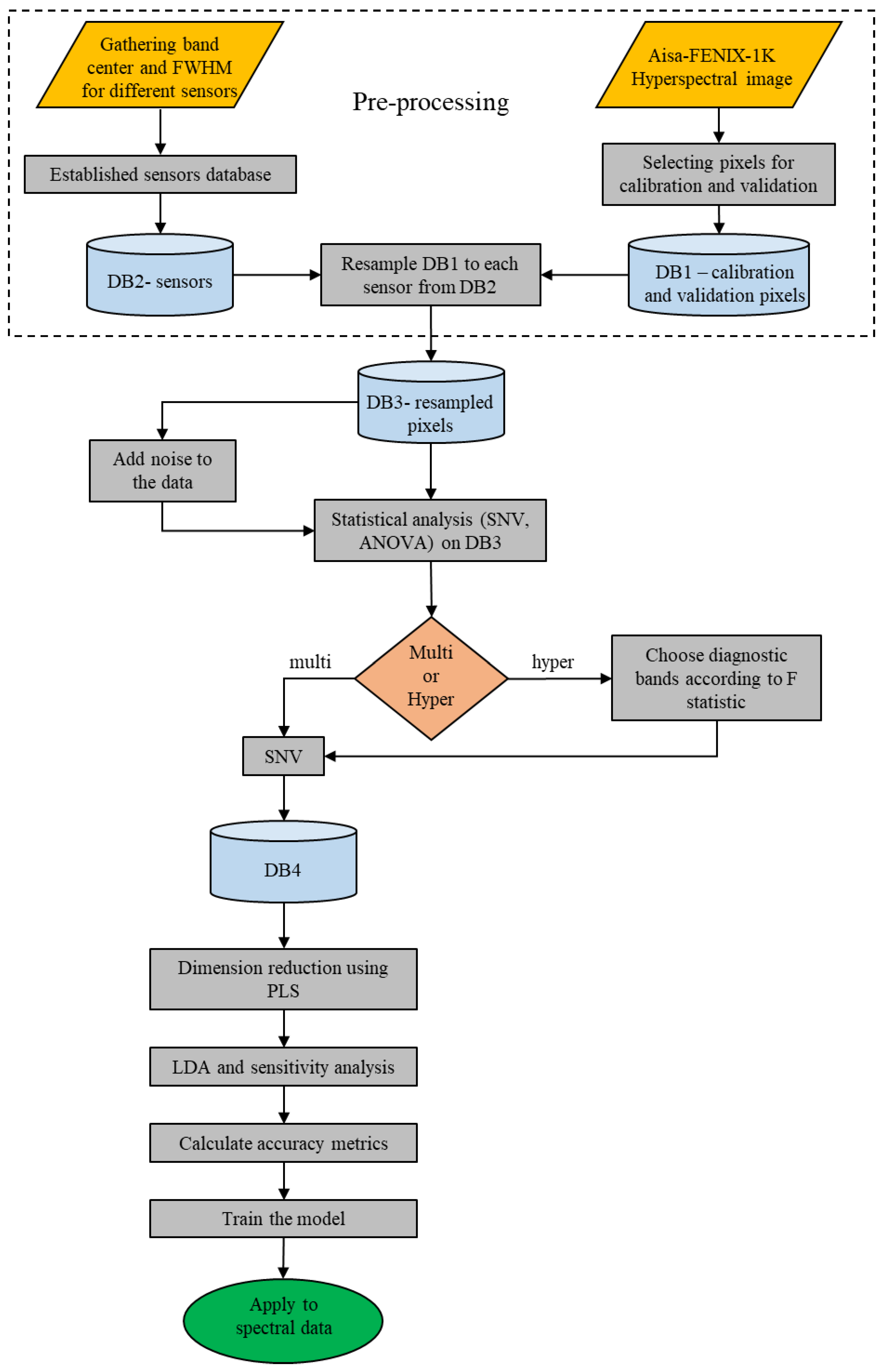
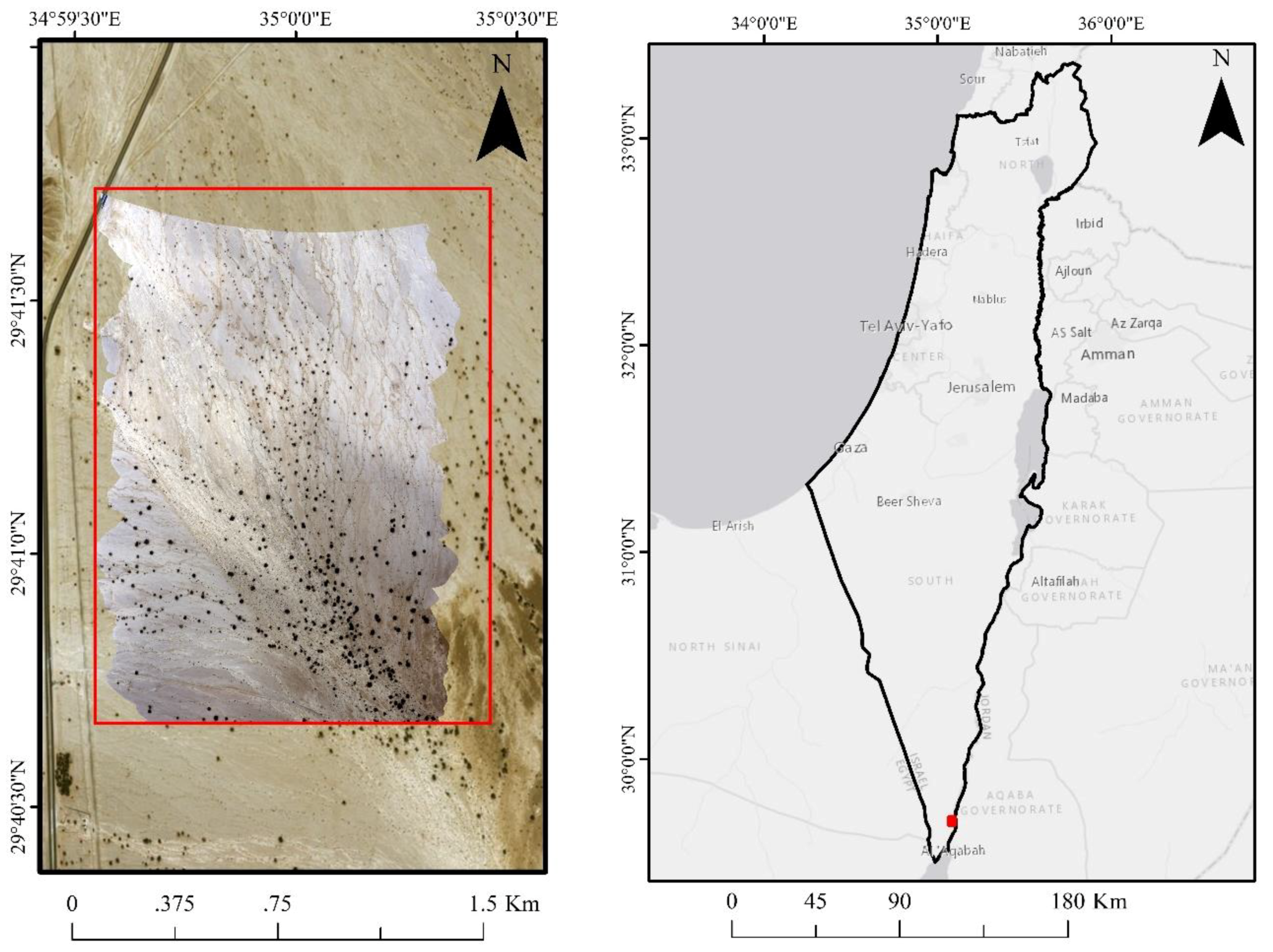
2.1. Study Flow Chart

The flow chart of this study is shown in Figure 1. The idea behind this was to use a spectral database to train a classifier (i.e., a machine learning model) on a low dimension data (i.e., spectral data with a low number of informative variables). During the process of model training, the model parameters (further explained) were optimized using various statistical methods. Once the parameters were set, the model performance was evaluated by applying it to a new dataset (i.e., validation set), and then to the hyperspectral image, thus producing classification maps. To evaluate these maps, they were visually compared to the original hyperspectral image in true-color composition, and the panchromatic Earth Resources Observation Satellite (EROS) image taken several days after the spill. The whole process was done automatically using an ad-hoc Python script.

2.2. Using a Machine Learning-Based Method

Any machine learning method is based on a training/calibration data which the machine learns from to identify connections and relationships within the data. Here, a set of calibration (1500 pixels) and validation (300 pixels) was used. This data contained oil-contaminated pixels (hereafter termed oil) and pixels containing zero contamination (hereafter termed clean). These pixels were manually selected from an AISA-FENIX 1K hyperspectral image with 1 m GSD. The calibration and validation pixels were selected by crossing information from in-situ visits and measurements, examining the Fenix hyperspectral image and an Earth Resources Observation Satellite (EROS) high-resolution (70 cm GSD) panchromatic image taken by Image Sat International—ISI, several days after an oil spill. By doing that the calibration and validation pixels could be chosen with high certainty. Although the focus of this study is the implementation of our model, rather than details regarding our published method, it is worth to mention that we chose clean pixels which looked similar both spectrally and visually to oil pixels (e.g., dark soil and dry vegetation).

The Fenix image was acquired in April 2017 over the Evrona Nature Reserve in southern Israel (Figure 2), approximately two and a half years after the occurrence of an unfortunate oil spill accident. In this accident, millions of liters of crude oil flowed into the Evrona Nature Reserve, spreading through the narrow and dry streaming channels characterizing the Reserve.

For more details regarding the oil spill, the acquisition and pre-processing of the Fenix image, and the pixels selection and location, the reader is referred to Section 2 in [7].

2.3. Sensors Database

We collected data regarding the band center and full width half maximum (FWHM) from various sources, as shown in

Table 1. The sensors used in this study.

Sensor Name in this Study	Sensor Full Name	Type	Number of Spectral Bands *	Spectral Range (nm) *	Source
Fenix	AisaFENIX 1K	Hyperspectral airborne	385	375–2500	http://www.specim.fi/downloads/AisaFenix-1K-ver1-2016.pdf
Hyperion	High resolution hyperspectral imager	Hyperspectral spaceborne	242	355–2500	https://www.indexdatabase.de/db/s-single.php?id=36
AVIRIS	The airborne visible/infrared imaging spectrometer	Hyperspectral airborne	224	374–2500	https://directory.eoportal.org/web/eoportal/airborne-sensors/aviris
HyMap	Hyperspectral Mapper	Hyperspectral airborne	126	453–2484	https://web.archive.org/web/20090410174538/http://www.aigllc.com/pdf/EARSEL98_HyMap.pdf
EnMap	The Environmental Mapping and Analysis Program	Hyperspectral spaceborne	244	424–2446	https://pdfs.semanticscholar.org/7d2e/c51c43d94a54ae01cab8d5d922c1a6684118.pdf
CASI	Compact Airborne Spectrographic Imager	Hyperspectral airborne	97	380–1050	http://www.itres.com/wp-content/uploads/2014/10/CASI-1500.pdf
ASTER	Advanced Spaceborne Thermal Emission and Reflection Radiometer	Multispectral space borne	9	560–2430	https://www.satimagingcorp.com/satellite-sensors/other-satellite-sensors/aster/
SN2	Sentinel-2	Multispectral spaceborne	11	442–2202	https://earth.esa.int/web/sentinel/technical-guides/sentinel-2-msi
VENUS **	Vegetation and Environment monitoring on a New Micro-Satellite	Multispectral spaceborne	11	420–920	https://directory.eoportal.org/web/eoportal/satellite-missions/v-w-x-y-z/venus
LS8	Landsat-8	Multispectral spaceborne	7	443–2200	https://directory.eoportal.org/web/eoportal/satellite-missions/l/landsat-8-ldcm#sensors
WV3	World View-3	Multispectral spaceborne	16	425–2330	https://directory.eoportal.org/web/eoportal/satellite-missions/v-w-x-y-z/worldview-3
Self	Self	Multispectral theoretical	6	1200–2350	Table 2 in this paper

* The number of spectral bands and the spectral range correspond to the data used in this study for resampling. Sensors might have different number of spectral bands and/or spectral range in different configuration modes. For more information, the reader is referred to the links provided under the ‘source’ column. ** The correct spelling is VENμS, but for convenience, it is spelled VENUS in this paper.

.

The data were organized to form a sensor database (see DB2 in Figure 1), which consisted of 11 different sensors, namely: multi- and hyperspectral air- and spaceborne sensors. The chosen sensors are well-known in the literature and are frequently used in studies. In other words, these sensors have been proven to work in practice, and thus represent “legitimate” spectral and spatial configuration.

The hyperspectral sensors obviously contain much more information than the multispectral, but in practice, this comes at the price of higher operational costs (for airborne), coarser GSD (for spaceborne), and more complex processing. Hence, multispectral sensors were also included in the data to examine whether they can deliver similar results to the hyperspectral ones. Three sensors in the database are currently not functioning, namely: ASTER, the high-resolution hyperspectral imager (Hyperion), and EnMap. The ASTER SWIR bands have been out of service since 2008, Hyperion was decommissioned at the beginning of 2017, and EnMap is not yet in orbit. Nevertheless, we decided to include them, as two of them were proven to function well in orbit, and EnMap is expected to be launched in the near future. An interesting choice was the Vegetation and Environment monitoring on a New Micro-Satellite (VENµS, hereafter termed VENUS; multispectral) and the Compact Airborne Spectrographic Imager (CASI; hyperspectral) sensors, because their spectral range is limited to ~400–1000 nm (visible-near-infrared—VNIR), as opposed to the other sensors (~400–2500 nm). Moreover, the diagnostic PHC-SFs are mainly found at ~1700 and ~2300 nm, which is not part of the spectral range of these sensors. This choice was made because of the nature of the machine learning approach taken here, which can find hidden connections between the spectra of the pixels to their class. In other words, as our method is based on a model that learns the spectral characteristics of each class without the use of any prior spectral knowledge, it was intriguing to see if it is possible to get good results with a limited spectral range. Additionally, we added a new sensor (Self;

Table 2. Specifications of the theoretical Self sensor. FWHM: full width half maximum.

Band Name	Min (nm)	Max (nm)	Band Center (nm)	FWHM (nm)
SWIR-1	1196.25	1228.75	1212.5	32.5
SWIR-2	1261.25	1293.75	1277.5	32.5
SWIR-3	1682.5	1707.5	1695	25
SWIR-4	1732.5	1757.5	1745	25
SWIR-5	2247.5	2282.5	2265	35
SWIR-6	2317.5	2352.5	2335	35

), which is a theoretical multi-spectral sensor with six bands in the SWIR spectral region. The band centers and FWHM of this sensor were defined according to the analysis of variance (ANOVA) results from [7], and are designed to overlap the PHC-SF

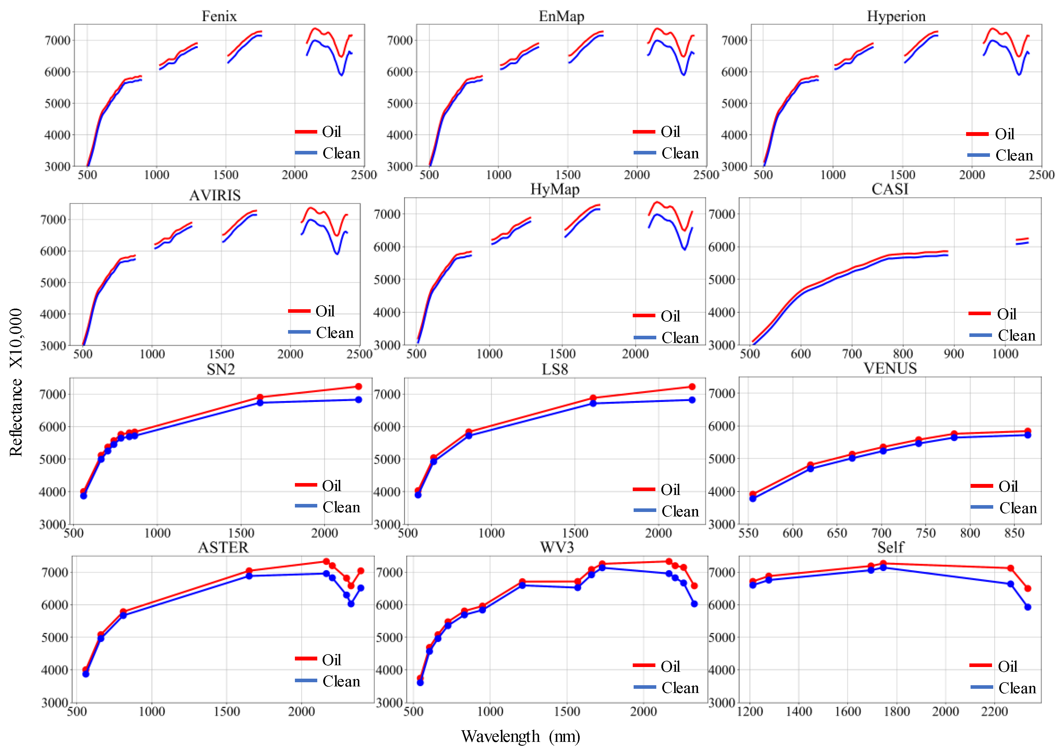
2.4. Spectral Resampling

Next, calibration and validation pixels (originated from the Fenix hyperspectral image) were spectrally resampled according to each sensor band center and FWHM and saved as a new (resampled) database (see DB3 in Figure 1). The resampling process was executed using Spectral Python, which is a Python library for processing spectral image data (http://www.spectralpython.net). In order to better illustrate the resampling process, Figure 3 shows an average spectrum (average of all clean and oil pixels in the DB3) per sensor. The spectra of the hyperspectral sensors are plotted continuously, while the spectra from the multispectral sensors are plotted segmentally, where each segment starts and ends with black dots, which represent the spectral band centers. For better visualization, the range of the values displayed on the axes in Figure 3 are sensor-specific (not identical for all sensors). The absorption features at approximately 2200 and 2300 nm stem from the presence of clay minerals and CaCO₃, respectively.

2.5. Calibrate the Machine Learning Model

The spectrally resampled database (which consists of resampled pixels per sensor) was standardized using standard normal variate (SNV) standardization [13], and then an analysis of variance (ANOVA) test was performed to understand which bands can be considered good separators between the two classes (clean or oil). The result of such a test is the F statistic, where a higher F statistic indicates better separation.

Then, the spectrally resampled database was subset to include only the bands that had an F statistic value above the threshold. SNV was applied to that database so as to create a new standardized database (see DB4 in Figure 1). For each sensor in DB4, a partial least squares (PLS) [14] model was used for dimension reduction, and the number of latent variables (LV) was selected according to the overall accuracy calculated from the cross-validation process. Then, linear discriminant analysis (LDA) [15] was applied to the LV of each sensor. LDA makes predictions by estimating the probability that a new set of inputs belongs to each class. The class that gets the highest probability threshold is the output prediction class. The default threshold is 50%, but here, an analysis was performed to choose the best probability threshold for each sensor, which optimized the metric accuracies. In other words, all the possible thresholds were examined, and the one that minimized the difference between the accuracy metrics was chosen. The accuracy metrics used here were the overall accuracy, the sensitivity, and the specificity:

$$OverallAccuracy=\frac{TP+TN}{TP+TN+FP+FN}$$

(1)

$$Sensitivity=\frac{TP}{TP+FN}$$

(2)

$$Specificity= \frac{TN}{TN+FP}$$

(3)

where TP (true positive) is the number of pixels correctly classified as oil, FP (false positive) is the number of pixels incorrectly classified as oil, TN (true negative) is the number of pixels correctly classified as clean, and FN (false negative) is the number of pixels incorrectly classified as clean. In addition, the Kappa coefficient (k) [16] was also calculated, because it is considered a more stringent metric, as it takes into account the possibility of agreement occurring by chance, as follows:

$$k= \frac{P_0-P_e}{1-P_e}$$

(4)

where P₀ is the relative observed agreement among the raters, and P_e is the hypothetical probability of chance agreement.

2.6. Validating and Testing the Model

From the calibration process, a set of sensor-specific model parameters was obtained, that is, the spectral bands above the F statistic threshold, the PLS linear transformation coefficients, the number of LV, the LDA coefficients, and the probability threshold. In other words, a model was created for each sensor based on the machine learning process, which found the best parameters for each sensor. Each model was applied to the corresponding sensor resampled validation database, to calculate the accuracy metrics (i.e., quantitative validation).

Then, to test the models, and to demonstrate how practical they are, the models were applied to the entire image, thus creating a series of thematic maps (a map for each sensor) that illustrate the predicted location of clean and oil pixels. Each map gave a broader view of the performances per sensor. Two scenes (one containing both oil and clean pixels, and the other containing only clean pixels) were selected in order to closely examine the classification results. These maps were later also spatially resampled (see spatial resampling under Results).

The testing process of the models was done qualitatively and not quantitatively (the reason for that is discussed further in the discussion part of this paper). This was done by visually evaluating and interpreting the agreement between the classified image to the Fenix true-color image and the EROS image.

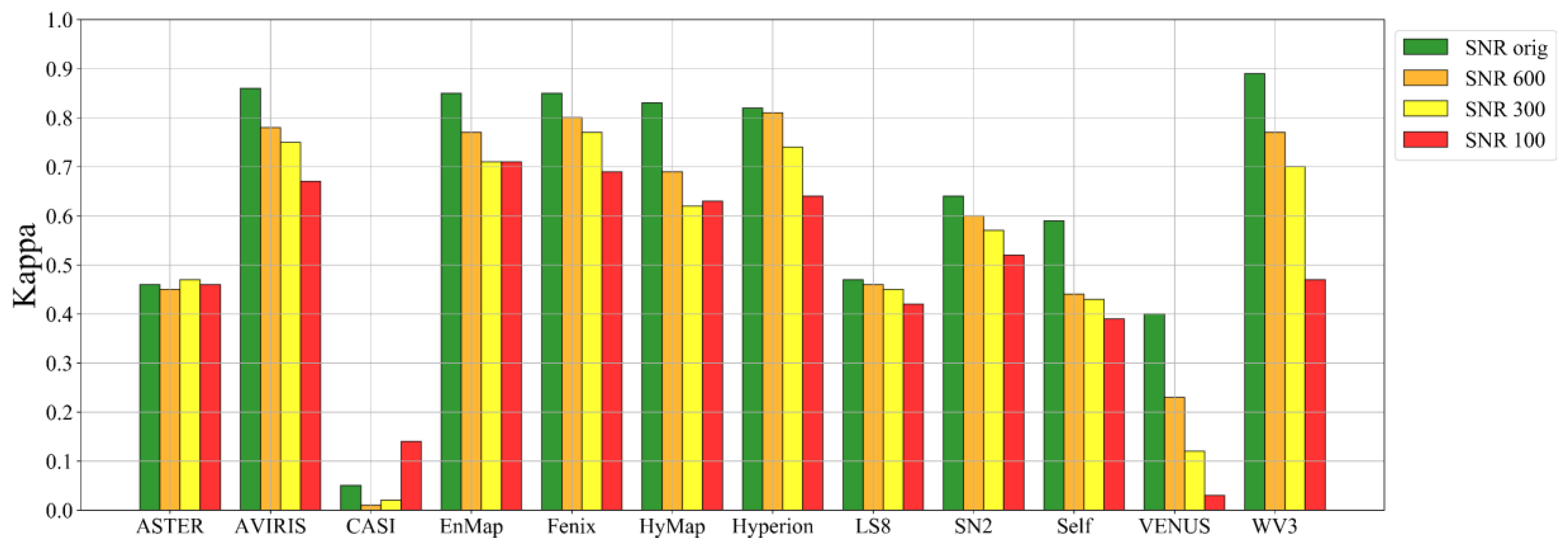
2.7. Add Noise to the Data

As explained, the calibration and validation data were based on pixels from the Fenix hyperspectral image of the Evrona Nature Reserve. The Fenix is considered to be a sensor with high performances and high SNR (see details in the link provided in Table 1). However, not all sensors have a similar SNR as the Fenix. Generally, SNR is an inherent character of the sensor itself and can vary depending on a collection of parameters, such as the sun angle and target reflectance. The performance of our method was tested here by adding scaled random Gaussian noise, relative to three SNR values, namely: low (100), moderate (300), and high (600). The noise was added according to Equation (12) in [17]:

$${\rho }_N=\rho \left(\lambda \right)\left[1+\frac{RAND\left(\lambda \right)}{SNR}\right]$$

(5)

where ρ_N(λ) is the reflectance spectrum with added noise at wavelength λ, ρ(λ) is the original resampled (to a specific sensor) noise-free spectrum at wavelength λ, RAND(λ) is a random number at wavelength λ from a Gaussian distribution with a mean of zero and standard deviation of one, and SNR is the desired SNR level. The Python algorithm was executed for each SNR level, and accuracy metrics were calculated for the validation database.

2.8. Spatial Resampling

Once the spectral resampling was done and the results were obtained, another examination was added to this study. Using ENVI 5.2 (Exelis Visual Information Solutions, Boulder, CO, USA), the original Fenix image (1 m GSD) was spatially resampled to 5, 7.5, 15, and 30 m. The resampling method was a pixel aggregate, which averages all of the pixel values that contribute to the output pixel. The 7.5 and 30 m GSD were chosen, as they correspond to WV3 (commercial delivery) and the general in-orbit hyperspectral sensors, respectively. The 5 and 15 m samples were selected to observe a more gradual change between the different GSDs. Then, the models (i.e., a model for each sensor with its specific parameters) were applied to the different GSD images, so as to observe to what extent the model is still useful.

In addition, another spatially resample process was executed for comparison (mentioned in Section 2.6) using the same technique mentioned. This process involved the thematic maps, which were based on the spectrally resampled original 1 m GSD image.

3. Results

3.1. Spectral Bands Selection

Figure 4 shows the F statistic for each band per sensor.

When examining the plots in Figure 4, one must pay attention to the values in the axes as they are different between sensors. For example, the F statistic values range from 0–200 (i.e., poor separation) for CASI, whereas for AVIRIS, these values range between 0–5000. The hyperspectral sensors (i.e., Fenix, EnMap, HyMap, AVIRIS, and Hyperion) demonstrate similar behavior, where three spectral areas can be distinguished as good separators, specifically, ~1250, 1730, and 2300 nm. These spectral ranges are associated with the spectral features of PHC and CaCO₃. The CASI sensor, which is also considered hyperspectral, does not contain information in these spectral regions. However, according to its ANOVA test, two alternative spectral regions (~550 and 750 nm) contain bands that are better separators than the other bands. Nevertheless, CASI’s F statistic values are low, which question its ability to perform well when applying to the entire image. The multispectral sensors show similarities and dissimilarities in comparison to the hyperspectral sensors. On the one hand, the SN2 and LS8 display bands in the SWIR as more important than in the other spectral regions. ASTER and WV3 demonstrate similar behavior and indicate the ~1700 nm region to be the most diagnostic region, and generally, WV3 has an affinity to the hyperspectral sensors. On the other hand, the 1700 nm region in Self seems to be the least important area compared to the other two spectral regions of PHC (i.e., 1200 and 2300 nm). This can be attributed to the spectral characteristics of Self. It has indeed spectral bands around the PHC-SF and therefore expected to perform similarly to ASTER and WV3 in terms of the ANOVA test. However, this is not exactly the case. A reason for that can be that its spectral bands are not perfectly located across the spectral range, in our case, and they do not completely overlap the spectral bands of ASTER and WV3. Because of that Self probably does not capture the most important spectral information, and hence, shows intermediate results (in terms of ANOVA) and different behavior from WV3.

VENUS, which only has spectral information up to 900 nm, exhibits two small peaks (~600 and 750 nm, uncompelling in terms of F statistic) similarly to CASI, which covers the same spectral range.

In the methodology described in [7], a threshold of F statistic = 1500 was set in order to decide for each band whether it was used or omitted from further analysis, to reduce the number of bands for further analysis (the main idea behind this step). The value of 1500 was originally selected because it captures peaks of the F statistic curve, allowing us to “cherry-pick” the good separators. However, this value was chosen for a hyperspectral sensor across the VNIR-SWIR, and here we had various sensors. If the same threshold was to apply to all sensors, then SN2, LS8, VENUS, and CASI would have zero bands left while ASTER, WV3, and Self would have one or two bands left for the analysis. In practice, applying a threshold of 1500 to all sensors would have left us only with hyperspectral sensors, which was not the intention as the merit of multispectral was also part of this study. Therefore, we decided that the 1500 threshold remained for the hyperspectral sensors excluding CASI (which covers a smaller spectral range), that had a threshold of 25 to capture its two F statistic peaks. No threshold was applied to the multispectral sensors.

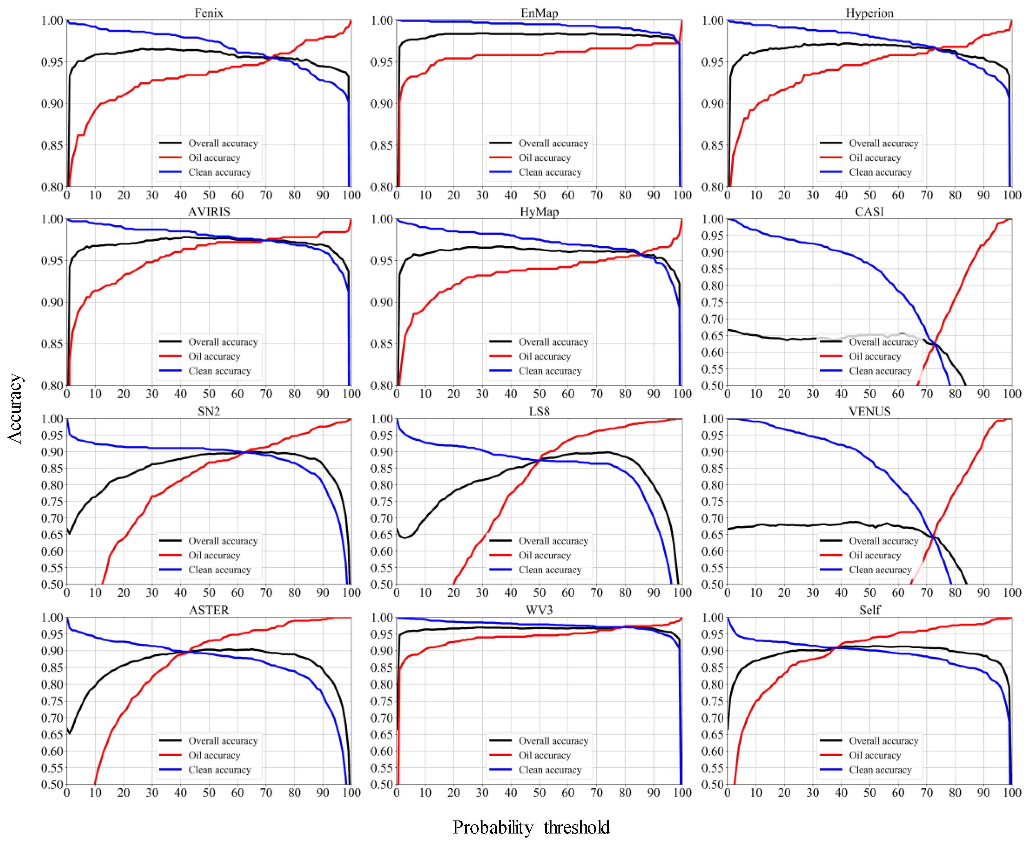
3.2. Selecting the Optimal Probability Threshold

The output of the LDA model is whether a pixel is contaminated with crude oil or whether it is uncontaminated. The final decision in such a model is based on the probability of a pixel to fit one of the classes, where the default probability is 50%. However, this default value does not necessarily give the ideal outcome. Figure 5 exhibits, per sensor, three accuracy metrics scores for each probability threshold, where the goal is to find the threshold values that minimize the differences between the metrics (i.e., the intersection point between the lines).

3.3. Cross-Validation and Validation

Table 3. Cross validation (Cal) and validation (Val) results from the spectral resample simulations.

Sensor.	Type	Best Threshold	Overall Accuracy		Sensitivity		Specificity		Kappa
			Cal	Val	Cal	Val	Cal	Val	Cal	Val
Fenix	Hyperspectral	72	0.95	0.93	0.95	0.91	0.96	0.94	0.90	0.85
EnMap	Hyperspectral	98	0.97	0.93	0.97	0.93	0.98	0.94	0.94	0.85
Hyperion	Hyperspectral	73	0.97	0.92	0.97	0.91	0.97	0.92	0.93	0.82
AVIRIS	Hyperspectral	69	0.97	0.94	0.97	0.91	0.97	0.95	0.94	0.86
HyMap	Hyperspectral	85	0.96	0.92	0.96	0.90	0.96	0.94	0.91	0.83
CASI	Hyperspectral	73	0.63	0.50	0.62	0.69	0.63	0.40	0.23	0.08
SN2	Multispectral	63	0.90	0.80	0.90	0.88	0.90	0.76	0.78	0.59
LS8	Multispectral	50	0.87	0.75	0.87	0.76	0.87	0.74	0.73	0.47
VENUS	Multispectral	72	0.64	0.72	0.64	0.65	0.64	0.76	0.26	0.40
ASTER	Multispectral	43	0.90	0.76	0.90	0.66	0.90	0.80	0.78	0.46
WV3	Multispectral	79	0.97	0.95	0.97	0.93	0.97	0.96	0.94	0.89
Self	Multispectral	38	0.91	0.84	0.91	0.77	0.91	0.87	0.80	0.64

summarizes the cross-validation and validation classification accuracies. Several outcomes can be drawn from this table.

First, the validation metrics are naturally lower than the cross-validation ones. Yet, the differences between the values are relatively small, which indicates a robust model. Second, the two sensors without bands in the SWIR spectral region (i.e., VENUS and CASI) have the lowest accuracy. Third, the hyperspectral sensors have superior results over the multispectral, with the prominent exception of WV3. Fourth, the Fenix sensor, with the highest number of spectral bands (i.e., has the most spectral information), does not stand out in terms of accuracy metrics. Fifth, all the hyperspectral sensors (and WV3) scores are closely akin. Sixth, WV3 (multispectral in the VNIR–SWIR) exhibits better results in comparison to its multispectral counterparts in the VNIR-SWIR (i.e., SN2, LS8, and ASTER). This is probably due to its spectral bands which are adequately located to “harvest” the important and diagnostic spectral information for the calibration set. Nevertheless, it is important to remember that this is a simulation, based on spectral resampling (where the other characteristics are of the Fenix sensor) aiming at demonstrating the potential of different sensors to perform well in a study site such as ours (see further Figure 6 for an example). Therefore, the results here should be interpreted as such. For example, the AVIRIS Kappa score in the validation is higher than the Fenix (0.85 versus 0.86). It does not mean that in practice AVIRIS will necessarily yield better results, rather that they have similar potential to achieve good classification results. Likewise, WV3 should not be considered to outperform the hyperspectral sensors (even if the exact numbers indicate that), rather to suggests its great potential of performing well in detecting PHC contamination as shown by [6].

Figure 6 shows the Kappa coefficient for all of the sensors in all of the added noise levels. The presented data correspond to the validation dataset (100 oil and 200 clean pixels). Almost all of the sensors have a better Kappa score with decreasing added noise, excluding CASI, which has especially low scores (see also Table 3) and thus can be considered unstable. Similarly, ASTER seems insensitive to added noise, but again, with low accuracy results. The sensors with the highest scores thus far (Fenix, AVIRIS, HyMap, Hyperion, EnMap, and WV3) stand out above the others, where even with the highest amount of noise, they still produce better scores than the others. The theoretical sensor (Self) displays moderate results, as well as SN2.

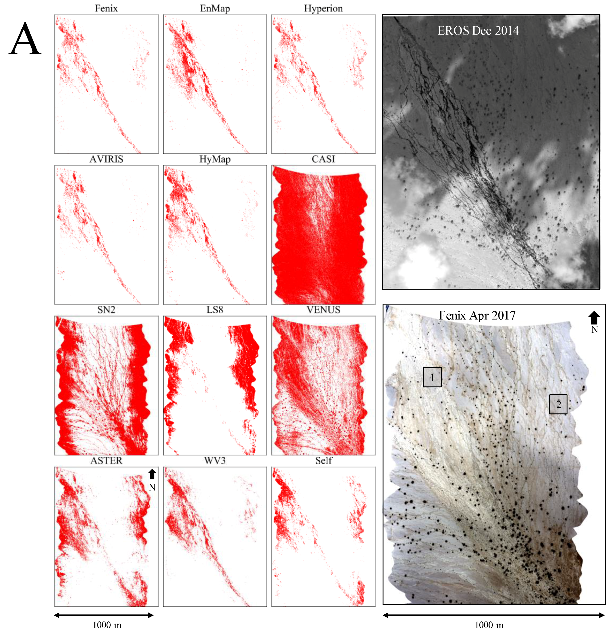
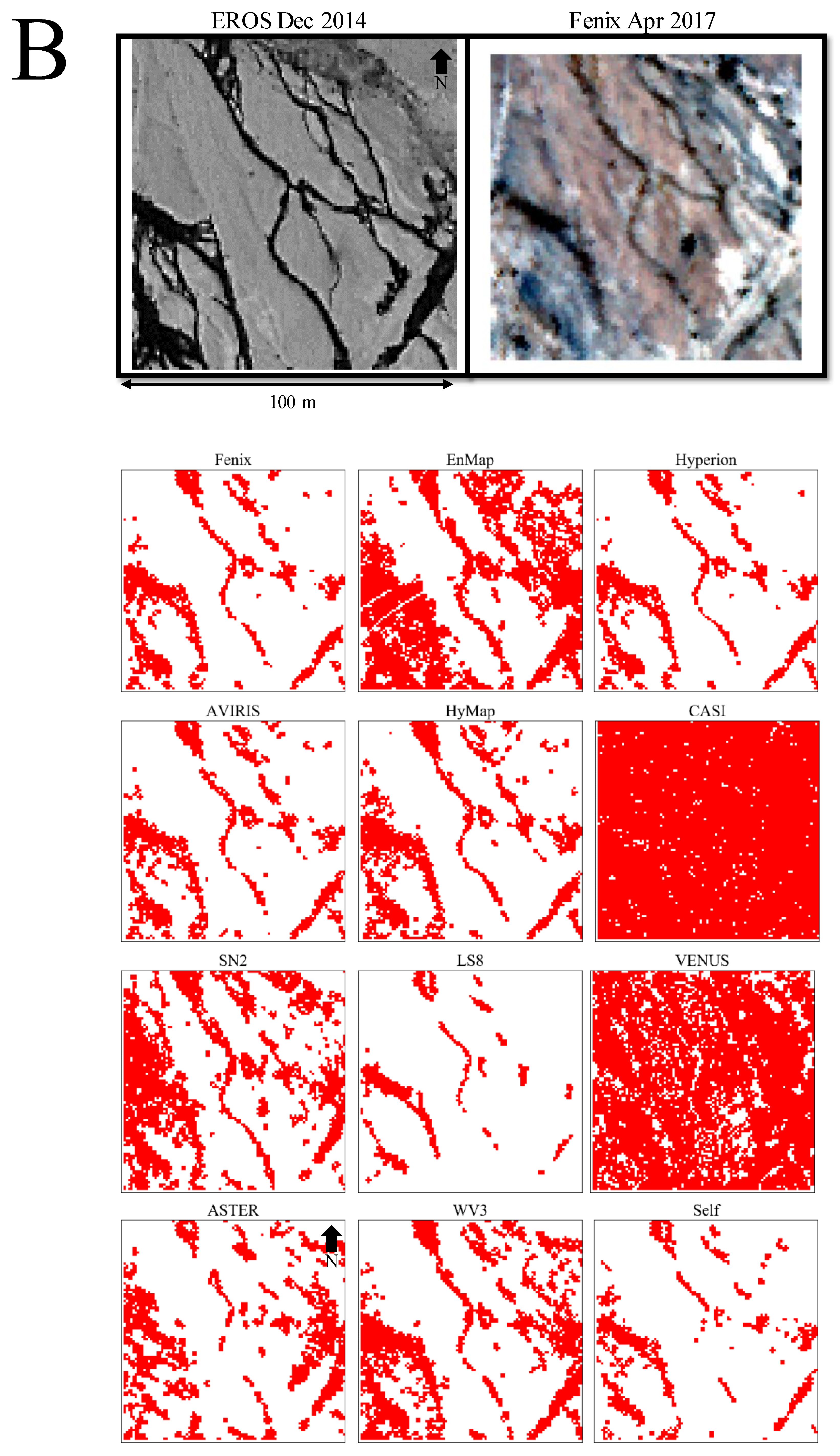
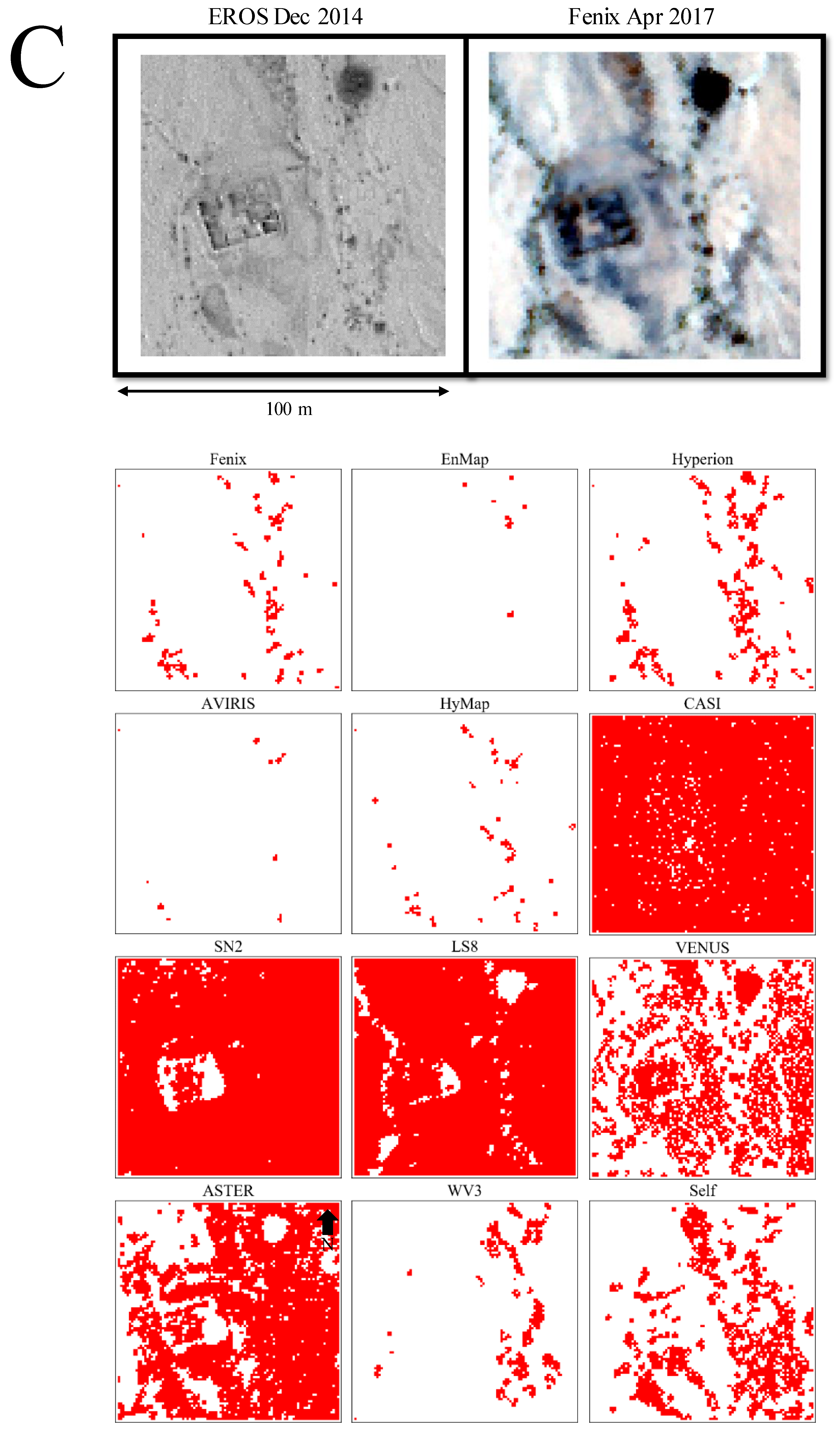
3.4. Model Predictions on the Image

3.4.1. Spectral Resampling

Figure 7 shows the model predictions for all of the simulations as a series of maps with white (clean) and red (oil) pixels. Figure 7 is divided into three panels, A, B, and C, which correspond to maps of the entire scene, maps for a specific contaminated zone, and maps for a specific uncontaminated zone, respectively. As implied by the results in Table 3 and Figure 5, the hyperspectral sensors (excluding CASI) and WV3 display similar classification schemes, which is in good agreement with the EROS image, whereas some multispectral sensors present unsatisfying classification maps (SN2 and LS8) and some (ASTER and Self) moderate results. It is important to mention that the surface of the Evrona Nature Reserve (covered in Figure 7A) is quite homogenous in terms of stream channels, vegetation, and soil compositions. According to Figure 7, one might consider that the classification follows the stream and not the oil; however, there are many similar uncontaminated streams that the models did not indicate them as contaminated. Additionally, most of the different light intensities in the true-color image (Figure 7A) are due to clouds. It also means that the stream channels that the oil flowed in are similar to the ones that the oil did not penetrate. In other words, the good agreement between the maps and the pattern of the spilled oil (also shown in Figure 12 in [7]) resulted from sensing the contamination itself and not from differences between the stream channels the oil “chose” to flow.

The main area of misclassification (i.e., oil predictions in clean areas) seems to be in the northeast part of the map, which is specifically dominant in ASTER, LS8, SN2, Self, and even Hyperion, Fenix, and WV3 to some extent. It is less observable in EnMap, AVIRIS, and HyMap.

This dominant misclassified area seems to occur on the boundaries of the image (it is nicely shown in ASTER, SN2, and LS8). A reason for this misclassification might be the off-nadir location of these pixels.

Figure 7B,C allow for a deeper evaluation of the model performances, where Figure 7B focuses on a specific zone (marked as 1 in panel A) with a clearly visible oil flow pattern, and Figure 7C centers over an uncontaminated zone. The hyperspectral sensors illustrate a prediction map, which is similarly close to the flow outlines depicted in the EROS image (acquired two and a half years before the hyperspectral Fenix image). EnMap seems to attain more false-positives (prediction oil when it should be clean) than its hyperspectral counterparts. In the multispectral domain, WV3, Self, and ASTER also demonstrate good agreement between the maps, where WV3 and ASTER seem to have a larger number of false-positives in a similar location to EnMap classification map. A surprising result is that the map produced by LS8 shows a nice clean outline of the spill. However, when observing the performance of LS8 in panel C, one can see that the LS8 model performed poorly, as all of the pixels in the image (in Panel C) ought to be white (i.e., clean). A similar phenomenon can be observed in ASTER and Self.

When evaluating the performances of the more competent sensors (in this study), EnMap seems to give a less satisfactory classification map in Panel B, but a much better one in Panel C. Judging by the two panels (B and C), AVIRIS appears to yield the best results. Nevertheless, this is a qualitative evaluation of two scenes. Overall, when observing Panel A, the results obtained by the hyperspectral sensors (excluding CASI) and WV3 seem to capture well the contamination pattern and the uncontaminated zones.

Figure 7 also nicely illustrates what was previously stated (in Section 3.3) regarding the interpretation of the quantitative validation results. The validation Kappa results indicate that WV3 has the best score. We stated that this score should not be interpreted as WV3 is better than the hyperspectral sensors, rather that it has great potential. Figure 7B, C proves that by showing that WV3 does not produce the best classification maps. It is more noticeable in Figure 7C which shows a scene with zero contamination, meaning that all red pixels (oil according to the model) are false-positive. There, WV3 seems to have a larger number of false-positives than the hyperspectral ones.

3.4.2. Spatial Resampling

As mentioned earlier, the original Fenix hyperspectral image was acquired with 1 m GSD, which is obviously not the same as all other sensors in this study. Hence, to examine the potential of the native GSD of the various sensors, the original 1 m GSD was resampled into four GSDs, namely: 5, 7.5, 15, and 30 m. Then, the models, which were developed per sensor in the previous section were applied to the different GSD images and the results are shown in column D in Figure 8. Additionally, Figure 8 also shows (for comparison purposes) three spatially resampled images: the true-color Fenix image, the EROS image, and the model predictions (from Figure 7A) in the columns A, B, and C, respectively. For illustration simplicity, we do not show here the spatially resampled maps of all of the sensors, but rather only for the Fenix. Naturally, as the GSD increases, the ability to classify the pixels correctly decreases, and the larger the area contaminated by the spill, the coarser the GSD that is needed for detection. With that being said, the spatial pattern of the spill outlined in the 1 m GSD is clearly observable in the 5 m map (column D), while this fades away in the 15 and 30 m maps. The 7.5 m GSD seems to be a transition GSD, with the ability to properly follow the oil spill pattern. Although it is not as good as the spectrally resampled 1 m prediction (column C), it does seem to enable following the oil spill.

The 15 and 30 GSD maps center on the larger area of the spill (the north-west part of the image). This does not mean that a GSD of 15 or 30 m are irrelevant to detect PHC, it just means that in our case study, where the oil flowed in narrow drainage channels, 15 or 30 m GSD will not be effective. It means that sensors with this GSD (e.g., LS8 and ASTER) are not suitable for this mission. This is somewhat compatible with the study done by [18], where they examined the ability to map minerals related to acid mine drainage and found the 15 m images to be comparable to the 2 m images, while the 30 m images lost the ability to identify smaller spectral features.

4. Discussion

The conditions under which this study was conducted were challenging. As the hyperspectral image was taken approximately long after an oil spill, it was difficult to clearly observe the contamination in the hyperspectral image, both visually and spectrally. Figure 7 and Figure 8 here, and Figure 7 in [7] demonstrate this challenge. Yet, the EROS image clearly depicts the “historic” outline of the spill. However, this outline of the spill from December 2014 cannot be fully quantitatively validated today, as there were some remediation efforts to minimize the spill which included pumping-out the oil. Moreover, the time gap of almost two and a half years between the spill and the Fenix hyperspectral image caused some of the oiled areas to be covered by a thin layer of sediments and dust. This can cause uncertainty if one would try to quantitatively assess the method results using recent data. Additionally, the nature of the spilled oil is another compelling reason for using a qualitative evaluation of the classification map as was done here. In our study site, the oil did not appear sporadically, for example in separated areas, rather flowed in continuous narrow channels. This means that in practice, the important thing is to detect the flow pattern rather than the number of oiled pixels in that pattern. Consider two scenarios where one is similar to ours and the other consists of oil that was dumped in several spatially unconnected locations. In the latter scene, failing to detect pixels in one of the dumping locations translates directly to contaminated areas that are not detected by remote sensing. Thus, detecting 50 locations out of 100, for example, means that the accuracy is 50%, and we missed 50 contamination sites. However, in the former scenario (i.e., ours) detecting 50 pixels that are spatially connected out of 100 pixels have the same 50% accuracy. However, here, the quantitative metric is less important because we did not miss the contaminated area, it is only “narrower”, containing fewer pixels, but it does delineate where the contamination is found.

The ANOVA results indicated the best bands that hold diagnostic spectral information to distinguish between oil and clean pixels. The bands for the hyperspectral sensors (excluding CASI) and WV3, and to some extent Self and ASTER, overlap with the PHC-SF as well as the CaCO₃ feature. This implies that the classification was based on the PHC effects on the spectrum of the underlying soil. However, these effects did not express themselves as one would expect (i.e., as the “classic” PHC features-see Figure 3 in [7]), but rather in smaller unobservable effects over the spectrum. The two sensors with the limited spectral range (CASI and VENUS) had very low F statistic values, which indicate that they probably do not hold any relevant information for the classification. The low accuracy metrics for these VNIR sensors, as well as the poor classification maps, proved this to be true. The other multispectral sensors showed moderate F statistic values, in comparison to the hyperspectral ones, which can be interpreted as not having sufficient spectral data to achieve good results. This was mainly shown in Figure 7. When considering the relatively coarse GSD of these sensors (LS8, SN2, and ASTER), we can deduce that they are not suitable for the classification needs of this study site.

The accuracy metrics from cross-validation and validation procedures as well as the classification maps (Figure 7) that resulted from spectral resampling clearly express the superiority of the hyperspectral sensors over multispectral ones in detecting PHC contamination in our study. This might sound obvious, but the results of WV3 suggest that a multispectral sensor, with adequately located spectral bands, can also achieve good results.

Despite minor differences in the cross-validation and validation accuracies between the hyperspectral sensors, we can infer that, in practice, there will be no compelling variation in the outcome of other hyperspectral sensors. This means that, in our case, such an ample amount of spectral data (Fenix-420 bands) is not mandatory for successful classification, and similar results can be obtained with half (AVIRIS; 224 bands) or even a third (HyMap; 126 bands) of the amount of these spectral bands.

These results do not mean that we can start and apply the models on these sensors, as it is mainly simulated data that correspond to 1 m GSD. The importance of these results is that our method can potentially be inclusive to spectral configurations other than the Fenix. This can be applied in practice, for example, when planning a flight mission or even a future sensor that will consist of spectral configuration, like one of the sensors that demonstrated good results here. Perhaps even a drone mission that can carry multispectral sensor with bands like WV3 can achieve good results in similar scenarios. However, this should be validated in future research.

The augmentation of our sensors database with two sensors that do not contain information in the PHC-SF proved that sensors with spectral information merely in the VNIR region are unsuitable for this kind of task. However, the results of Self, which has only bands in the SWIR, in comparison with WV3, imply that for multispectral sensors, the VNIR range might hold some relevant information to discriminate between clean and oil pixels.

When examining the classification maps produced by the models (especially the ones resulting from the hyperspectral sensors), one might suspect that the classification was based on the mineralogy of the streams and not on the oil spill. Naturally, the oil flowed in the narrow streams of the Reserve and not otherwise. However, as the results indicate, the classification was based on the effect of PHC on the spectrum and the Reserve has many other streams with similar mineralogy composite where the oil did not flow. These streams can be found in the vicinity of the streams that the oil did flow in as well as streams far from it (mainly in the eastern part of the scene). These streams can be seen in Figure 7, and in Figures 8, 11 and 12 in [7]. Notwithstanding, the classification maps focused on the streams where the oil flowed and not in different ones.

The spectral simulation for the hyperspectral spaceborne (i.e., EnMap and Hyperion) resulted in high accuracy metrics and a good agreement of the classification maps to the true-color and EROS images, as well as to the other airborne hyperspectral classification maps. Still, when examining their performance considering their native spatial resolution (i.e., 30 m), the classification map does not capture the entire contamination pattern. EnMap and Hyperion have similar spectral and spatial characteristics to future spaceborne hyperspectral instruments; therefore, we can deduce that because of their GSD (30 m), they will not be useful in scenarios like ours. Reference [18] found that 30 m GSD will be sufficient in identifying potentially hazardous acid mine drainage features that cover large areas of at least 75 m in width, which is different from the narrow stream channels in our study site.

Overall, when considering all of the parameters (e.g., spectral, spatially, and practicality) required for the task presented in this study, it seems that WV3 might have the characteristics that balance the best between these parameters. It is a multispectral sensor operating in space, with adequately located SWIR bands for PHC-SF detection that collect enough spectral information. This is compatible with the study done by [6], which found the SWIR bands of WV3 to be adequate for PHC detection when the PHC-SF are clearly observable. Additionally, GSD of 7.5 m seems to still capture the outline of the spill, even if it is segmented in some places. This is compatible with [4], who used AVIRIS data in 3.5 and 7.6 m GSD, and had a high accuracy in detecting PHC-SF in marshes following the Deepwater Horizon incident, and with [18], who concluded that a GSD of 2–15 m is required for the identification of acid mine drainage in smaller features such as stream channels and acidic springs/seeps.

It is worth mentioning that the currently new generation of orbital hyperspectral sensor with 10 m GSD is planned by both the Italian and the Israeli space agencies—“SHALOM”—which is a sensor with 224 bands across 400–2500 nm with a high SNR. It is more likely to assume that SHALOM will serve as an adequate tool to detect PHC–SF from space, and accordingly, may add important applications to the already existing application list issued of SHALOM [19].

It is important to distinguish between the models developed in this paper and their corresponded sensor-specific parameters, and the method (the concept/approach). The method suggests an approach to analyze and classify spectral data, specifically hyperspectral data. This method was developed for cases where the spectral features of a target are not clearly visible in the spectrum or are not as one would expect. This is in contrast to many other studies that showed the expected PHC-SF in their hyperspectral measurements [3,20,21,22,23,24]. The method here is not limited to a specific spectral or spatial resolution, it is not limited to crude oil or other contaminant or target, it is an approach we believe can be generalized. This method was developed because the classic/traditional methods (such as spectral angle mapper, continuum removal, derivatives, slopes, indices) completely failed in our case.

The models here are sensor-specific, and probably also site and crude oil specific. The coefficients and parameters of each model are a result of applying our method to each sensor. We have developed this method on data from our test site (Evrona Nature Reserve oil spill), but the oil spill can be considered as a case study for our approach. Hence, the models are limited and might be site/contaminant-specific but not the method.

Therefore, we believe that the method (and not a specific model) should be the focus of this study and can be inclusive to other scenarios, as it is not sensor-specific or even oil- or soil-specific, and no prior spectral knowledge is required. Even in scenarios where the spectral features of oil are visible, our method can be applied and might even have better results in comparison with the methods that are based on prior spectral knowledge, since our method can find better patterns in the data.

On one hand, our method does require some knowledge regarding the location of contaminated and clean targets to calibrate the model, which can be considered a limitation. We used 1800 pixels to train and validate the models and made predictions on over 2 million pixels. On the other hand, if one would have analyzed the Fenix image used in this study by looking for the appearance of the diagnostic PHC-SF, his/her conclusion would be that the entire image is PHC-free, which is obviously not the case.

The results should also be considered more broadly than just for the specific sensors used in this study. The sensors represent a variety of operational instruments both from the air and from space. Hence, it should not be interpreted merely as which sensor can be immediately used, rather what are the better spectral and spatial configurations, as well as the limitation for such a challenging study case shown here.

The method we applied here should be further investigated in other real scenarios (as opposed to controlled condition), including different types of soil and contaminant, because the type of soil affects the ability to spectrally detect constituents and contaminants, as shown elsewhere [25,26].

5. Conclusions

This study broadened the applicability of a recently published study [7], which successfully utilized a machine learning approach to detect crude oil contamination, in challenging conditions, two and a half years after an oil spill incident. This was done by simulating an assortment of spectral and spatial configurations, which correspond to multi- and hyperspectral air- and spaceborne sensors. The base for the simulations was an AISA-FENIX 1K airborne hyperspectral image with 1 m GSD, which was used to classify contaminated and uncontaminated pixels without prior spectral knowledge.

All of the hyperspectral sensors, simulated here, which measure the spectrum from 400 to 2500 nm, were found to contain enough spectral information to appropriately discriminate between the contaminated and uncontaminated pixels. Based on the simulations, it was also found that a large number of spectral bands (420 in the AisaFenix-1k sensor) might not be essential since a smaller number of spectral bands (126 in AVIRIS) showed similar classification results. The sensors that measure the spectrum from 400 to 1000 nm, were found to be irrelevant for detecting crude oil contamination in challenging conditions. Although the hyperspectral sensors produced good results, and naturally captured greater amounts of spectral information, it was found that WorldView-3 (a multispectral sensor) has great potential to achieve good results in detecting crude oil contamination.

The implications of this study are the following: in cases where the expected spectral feature of constituents (e.g., contaminants) are not clearly seen in the spectrum, our approach can be utilized, regardless of the sensor and site types, so as to potentially disclose the location of the contaminant.

References

1. Cloutis, E.A. Spectral reflectance properties of hydrocarbons: Remote-sensing implications. Science 1989, 245, 165–168. [Google Scholar] [CrossRef]
2. Ellis, J.M.; Davis, H.H.; Zamudio, J.A. Exploring for onshore oil seeps with hyperspectral imaging. Oil Gas J. 2001, 99, 49–56. [Google Scholar]
3. Horig, B.; Kuhn, F.; Oschutz, F.; Lehmann, F. HyMap hyperspectral remote sensing to detect hydrocarbons. Int. J. Remote Sens. 2001, 22, 1413–1422. [Google Scholar] [CrossRef]
4. Kokaly, R.F.; Couvillion, B.R.; Holloway, J.M.; Roberts, D.A.; Ustin, S.L.; Peterson, S.H.; Khanna, S.; Piazza, S.C. Spectroscopic remote sensing of the distribution and persistence of oil from the Deepwater Horizon spill in Barataria Bay marshes. Remote Sens. Environ. 2013, 129, 210–230. [Google Scholar] [CrossRef]
5. Pabon, R.E.C.; de Souza Filho, C.R.; de Oliveira, W.J. Reflectance and imaging spectroscopy applied to detection of petroleum hydrocarbon pollution in bare soils. Sci. Total Environ. 2019, 649, 1224–1236. [Google Scholar] [CrossRef]
6. Asadzadeh, S.; de Souza Filho, C.R. Investigating the capability of WorldView-3 superspectral data for direct hydrocarbon detection. Remote Sens. Environ. 2016, 173, 162–173. [Google Scholar] [CrossRef]
7. Pelta, R.; Carmon, N.; Ben-Dor, E. A machine learning approach to detect crude oil contamination in a real scenario using hyperspectral remote sensing. Int. J. Appl. Earth Obs. Geoinf. 2019, 82, 101901. [Google Scholar] [CrossRef]
8. Guanter, L.; Kaufmann, H.; Segl, K.; Foerster, S.; Rogass, C.; Chabrillat, S.; Kuester, T.; Hollstein, A.; Rossner, G.; Chlebek, C.; et al. The EnMAP Spaceborne Imaging Spectroscopy Mission for Earth Observation. Remote Sens. 2015, 7, 8830–8857. [Google Scholar] [CrossRef]
9. Natale, V.G.; Kafri, A.; Tidhar, G.A.; Chen, M.; Feingersh, T.; Sagi, E.; Cisbani, A.; Baroni, M.; Labate, D.; Nadler, R.; et al. SHALOM–Space-borne hyperspectral applicative land and ocean mission. In Proceedings of the 2013 5th Workshop on Hyperspectral Image and Signal Processing: Evolution in Remote Sensing (WHISPERS), Gainesville, FL, USA, 26–28 June 2013; pp. 1–4. [Google Scholar]
10. Pignatti, S.; Palombo, A.; Pascucci, S.; Romano, F.; Santini, F.; Simoniello, T.; Umberto, A.; Vincenzo, C.; Acito, N.; Diani, M.; et al. The PRISMA hyperspectral mission: Science activities and opportunities for agriculture and land monitoring. In Proceedings of the 2013 IEEE International Geoscience and Remote Sensing Symposium-IGARSS, Victoria, Australia, 21–26 July 2013; pp. 4558–4561. [Google Scholar]
11. Iwasaki, A.; Ohgi, N.; Tanii, J.; Kawashima, T.; Inada, H. Hyperspectral Imager Suite (HISUI)-Japanese hyper-multi spectral radiometer. In Proceedings of the 2011 IEEE International Geoscience and Remote Sensing Symposium, Sendai, Japan, 1–5 August 2011; pp. 1025–1028. [Google Scholar]
12. Nieke, J.; Rast, M. Towards the Copernicus Hyperspectral Imaging Mission For The Environment (CHIME). In Proceedings of the IGARSS 2018–2018 IEEE International Geoscience and Remote Sensing Symposium, Valencia, Spain, 22–27 July 2018; pp. 157–159. [Google Scholar]
13. Barnes, R.J.; Dhanoa, M.S.; Lister, S.J. Standard Normal Variate Transformation and De-trending of Near-Infrared Diffuse Reflectance Spectra. Appl. Spectrosc. AS 1989, 43, 772–777. [Google Scholar] [CrossRef]
14. Wold, S.; Sjostrom, M.; Eriksson, L. PLS-regression: a basic tool of chemometrics. Chemom. Intell. Lab. Syst. 2001, 58, 109–130. [Google Scholar] [CrossRef]
15. Fisher, R.A. The Use of Multiple Measurements in Taxonomic Problems. Ann. Eugen. 1936, 7, 179–188. [Google Scholar] [CrossRef]
16. Cohen, J. A coefficient of agreement for nominal scales. Educ. Psychol. Meas. 1960, 20, 37–46. [Google Scholar] [CrossRef]
17. Rodger, A.; Laukamp, C.; Haest, M.; Cudahy, T. A simple quadratic method of absorption feature wavelength estimation in continuum removed spectra. Remote Sens. Environ. 2012, 118, 273–283. [Google Scholar] [CrossRef]
18. Davies, G.E.; Calvin, W.M. Mapping acidic mine waste with seasonal airborne hyperspectral imagery at varying spatial scales. Environ. Earth Sci. 2017, 76, 432. [Google Scholar] [CrossRef]
19. Feingersh, T.; Dor, E.B. SHALOM–A Commercial Hyperspectral Space Mission. In Optical Payloads for Space Missions; Feingersh, T., Dor, E.B., Qian, S.-E., Eds.; John Wiley and Sons, Ltd.: Hoboken, NJ, USA, 2015; pp. 247–263. [Google Scholar]
20. Khanna, S.; Santos, M.J.; Ustin, S.L.; Koltunov, A.; Kokaly, R.F.; Roberts, D.A. Detection of Salt Marsh Vegetation Stress and Recovery after the Deepwater Horizon Oil Spill in Barataria Bay, Gulf of Mexico Using AVIRIS Data. PLoS ONE 2013, 8, e78989. [Google Scholar] [CrossRef]
21. Peterson, S.H.; Roberts, D.A.; Beland, M.; Kokaly, R.F.; Ustin, S.L. Oil detection in the coastal marshes of Louisiana using MESMA applied to band subsets of AVIRIS data. Remote Sens. Environ. 2015, 159, 222–231. [Google Scholar] [CrossRef]
22. Scafutto, R.D.M.; de Souza Filho, C.R.; de Oliveira, W.J. Hyperspectral remote sensing detection of petroleum hydrocarbons in mixtures with mineral substrates: Implications for onshore exploration and monitoring. ISPRS J. Photogramm. Remote Sens. 2017, 128, 146–157. [Google Scholar] [CrossRef]
23. Scafutto, R.D.M.; de Souza Filho, C.R.; Rivard, B. Characterization of mineral substrates impregnated with crude oils using proximal infrared hyperspectral imaging. Remote Sens. Environ. 2016, 179, 116–130. [Google Scholar] [CrossRef]
24. Kuhn, F.; Oppermann, K.; Horig, B. Hydrocarbon Index–An algorithm for hyperspectral detection of hydrocarbons. Int. J. Remote Sens. 2004, 25, 2467–2473. [Google Scholar] [CrossRef]
25. Ogen, Y.; Neumann, C.; Chabrillat, S.; Goldshleger, N.; Ben Dor, E. Evaluating the detection limit of organic matter using point and imaging spectroscopy. Geoderma 2018, 321, 100–109. [Google Scholar] [CrossRef]
26. Pelta, R.; Ben-Dor, E. Assessing the detection limit of petroleum hydrocarbon in soils using hyperspectral remote-sensing. Remote Sens. Environ. 2019, 224, 145–153. [Google Scholar] [CrossRef]
Figure 1. Flow chart that demonstrates the methodology of this study.
Applsci 09 05151 g001
Figure 2. The location of the study is in southern Israel. The extent of the Fenix hyperspectral image is shown in the red rectangular.
Applsci 09 05151 g002
Figure 3. Average spectrum of clean and oil per sensor after spectral resampling. The spectra of the hyperspectral sensors are plotted as a continuous line, while the black dots in the spectra of the multispectral sensors represent the band centers. Please note that the x-axis represents the specific wavelengths for each sensor.
Applsci 09 05151 g003
Figure 4. Analysis of variance (ANOVA) test results for all of the sensors. Three spectral regions, which are above the F statistic threshold, marked with red circles in the Fenix plot and denoted as 1, 2, and 3, correspond to petroleum hydrocarbons (PHC), clay minerals, and CaCO3 spectral features, respectively. Please note that the x-axis represents the specific wavelengths for each sensor and pay attention to the F statistic values in each plot.
Applsci 09 05151 g004
Figure 5. Optimizing the probability threshold for each sensor.
Applsci 09 05151 g005
Figure 6. Validation results for all of the sensors with all levels of additive noise.
Applsci 09 05151 g006
Figure 7. Model prediction (spectral resampling) for all of the sensors together with an EROS image (several days after the spill) and Fenix true color (two and a half years after the spill). Red pixels represent oil and white pixels represent clean. (A)—An overview of the entire study area. The areas denoted as 1 and 2 correspond to the scenes shown in (B) (contaminated scene) and (C) (uncontaminated scene), respectively. (B)—A scene with a clear outline of the oil contamination in narrow stream channels, which helps to appreciate the model performances. (C)—A scene with a relatively large amount of false positive (prediction of oil where it should be clean). Note that these maps are in 1 m GSD.
Applsci 09 05151 g007aApplsci 09 05151 g007bApplsci 09 05151 g007c
Figure 8. Model prediction (only for the Fenix sensor) resulted from the spatial resampling. (A)—Evrona true color composite, resampled to different GSD. (B)—EROS image, resampled to different GSD. (C)—Predictions based on the original GSD, resampled to various GSDs. (D)—Prediction made on the spatially resampled hyperspectral image.
Applsci 09 05151 g008