Optical Soliton Solutions of the Cubic-Quartic Nonlinear Schrödinger and Resonant Nonlinear Schrödinger Equation with the Parabolic Law

Featured Application

The optical soliton solutions obtained in this research paper may be of concern and useful in many fields of science, such as mathematical physics, applied physics, nonlinear science, and engineering.

Abstract

In this paper, the cubic-quartic nonlinear Schrödinger and resonant nonlinear Schrödinger equation in parabolic law media are investigated to obtain the dark, singular, bright-singular combo and periodic soliton solutions. Two powerful methods, the $\left(m+\frac{G^{\prime }}{G}\right)$ improved expansion method and the exp$\left(-\phi \left(\xi \right)\right)$ expansion method are utilized to construct some novel solutions of the governing equations. The obtained optical soliton solutions are presented graphically to clarify their physical parameters. Moreover, to verify the existence solutions, the constraint conditions are utilized.

1. Introduction

In the current century, many entropy problems have been expressed by using mathematical models that are nonlinear partial differential equations. New results in the last few years have shown that the relation between non-standard entropies and nonlinear partial differential equations can be applied on new nonlinear wave equations inspired by quantum mechanics. Nonlinear models of the celebrated Klein–Gordon and Dirac equations have been found to admit accurate time dependent soliton-like solutions with the shapes of the so-called q-plane waves. Such q-plane waves are generalizations of the complex exponential plane wave solutions of the linear Klein–Gordon and Dirac equations [1]. Wave progressing of soliton forming and its application in the differential equation has been noticeable in the last few years. The physical phenomena of nonlinear partial differential equations (NLPDEs) may connect to many areas of sciences, for example plasma physics, optical fibers, nonlinear optics, fluid mechanics, chemistry, biology, geochemistry, and engineering sciences. The nonlinear Schrödinger equations describe wave propagation in optical fibers with nonlinear impacts [2,3,4].

Various numeric and analytic techniques have been used to seek solutions for nonlinear differential equations such as the homotopy perturbation scheme [5], the Adams–Bashforth–Moulton method [6], the shooting technique with fourth-order Runge–Kutta scheme [7,8,9,10], the group preserving method [11], the finite forward difference method [12,13], the Adomian decomposition method [14,15], the sine-Gordon expansion method [16,17,18], the modified auxiliary expansion method [19], the modified exp$\left(-\phi \left(\xi \right)\right)$ expansion function method [20,21], the improved Bernoulli sub-equation method [22,23], the Riccati–Bernoulli sub-ODE method [24], the modified exponential function method [25], the improved tan$\left(\varphi \left(\xi \right)/2\right)$ [26,27], the Darboux transformation method [28,29], the double $\left(\frac{G^{\prime }}{G},\frac{1}{G^{\prime }}\right)$ expansion method [30,31], the $\left(\frac{1}{G^{\prime }}\right)$ expansion method [32,33], the decomposition Sumudu-like-integral transform method [34], and the inverse scattering method [35].

In recent years, many researchers have carried out investigations on the governing models in optical fibers. The nonlinear Schrödinger equation, involving cubic and quartic-order dispersion terms, has been investigated to seek the exact optical soliton solutions via the undetermined coefficients method [36], the modified Kudryashov approach [37], the complete discrimination system method [38], the generalized tanh function method [39], the sin-cosine method, as well as the Bernoulli equation approach [40], the semi-inverse variation method [41], a simple equation method [3], and the extended sinh-Gordon expansion method [42].

Now, optical solitons are the exciting research area of nonlinear optics studies, and this research field has led to tremendous advances in their extensive applications. It is identified that the dynamics of nonlinear optical solitons and Madelung fluids are based on the generalized nonlinear Schrödinger dispersive equation and resonant nonlinear Schrödinger dispersive equation. In the research of chirped solitons in Hall current impacts in the field of quantum mechanics, a specific resonant term must be given [43].

Dispersion and nonlinearity are the two key elements for the propagation of solitons over intercontinental ranges. Normally, group velocity dispersion (GVD) leveling with self-phase modulation in a sensitive way allows such solitons to maintain long distance travel. Now, it could occur that GVD is minuscule and therefore completely overlooked, so in this condition, the dispersion impact is rewarded for by third-order (3OD) and fourth-order (4OD) dispersion impacts. This is generally referred to as solitons that are cubic-quartic (CQ). This term was implemented in 2017 for the first time. This model was later extensively researched through different points of view such as the semi-inverse variation principle [41], Lie symmetry [44], conservation rules [45], and the system of undetermined coefficients [37]. Consider the nonlinear Schrödinger and resonant nonlinear Schrödinger equations in the appearance of 3OD and 4OD without both GVD and disturbance. The equations are as follows:

$$i{u}_t+i\alpha u_{xxx}+\beta u_{xxxx}+cF\left({\left|u\right|}^2\right)u=0,$$

(1)

$$i{u}_t+i\alpha u_{xxx}+\beta u_{xxxx}+cF\left({\left|u\right|}^2\right)u+c_3\left(\frac{{\left|u\right|}_{xx}}{\left|u\right|}\right)u=0.$$

(2)

In Equations (1) and (2), $u\left(x,t\right)$ is the complex valued wave function and x (space) and t (time) are independent variables. The coefficients $\alpha$ and $\beta$ are real constants, while $c_3$ is the Bohm potential that occurs in Madelung fluids. The Bohm potential term of disturbance generates quantum behavior, so that quantum characteristics are closely related to their special characteristics. Therefore, we have the chirped NLSE’s disturbance expression giving us the introduction of the theory of hidden variables. Therefore, it will be more crucial to retrieve accurate solutions for the development of quantum mechanics from disturbed chiral (resonant) NLSE [46]. Furthermore, the functional F is a real valued algebraic function that represents the source of nonlinearity and $F\left({\left|u\right|}^2\right)u:C\to C$. In more detail, the function $F\left({\left|u\right|}^2\right)u$ is p-times continuously differentiable, so that:

$$\begin{array}{l}\hfill F\left({\left|u\right|}^2\right)u\in {\displaystyle \bigcup _{m,n=1}^{\infty }}{C}^p\left(\left(-n,n\right)\times \left(-m,m\right):R^2\right).\end{array}$$

Suppose that $F\left(u\right)={\mathrm{c}}_{1}u+c_2{u}^2$, so Equations (1) and (2) can be rewritten as:

$$i{u}_t+i\alpha u_{xxx}+\beta u_{xxxx}+\left(c_1{\left|u\right|}^2+c_2{\left|u\right|}^4\right)u=0,$$

(3)

$$i{u}_t+i\alpha u_{xxx}+\beta u_{xxxx}+\left(c_1{\left|u\right|}^2+c_2{\left|u\right|}^4\right)u+c_3\left(\frac{{\left|u\right|}_{xx}}{\left|u\right|}\right)u=0.$$

(4)

Equation (3) was investigated by making $c_2=0$ in [47] via the Kudryashov approach. The conservation laws to obtain the conserved densities for Schrödinger’s nonlinear cubic-quarter equation have been analyzed in Kerr and power-law media [45]. The undetermined coefficients method has been employed to construct bright soliton and singular soliton solutions of Equation (1), when nonlinearity has been taken into consideration in the instances of the Kerr law and power law [37]. In this study, we use two methods to investigate soliton solutions of the cubic-quartic nonlinear Schrödinger equation and cubic-quartic resonant nonlinear Schrödinger equation with the parabolic law, namely Equations (3) and (4).

2. Instructions for the Methods

Assume a nonlinear partial differential equation (NLPDE) as follows:

$$P\left(U,U_x,U_t,U_{xx},U_{tt},U_{tx}, \dots \right)=0,$$

(5)

and define the traveling wave transformation as follows,

$$U\left(x,y,t\right)=\varphi \left(\zeta \right),\zeta =x-\nu t.$$

(6)

Putting Equation (6) into Equation (5), the outcome is:

$$N\left(\varphi ,{\varphi }^{\prime },{\varphi }^{″},\dots \right)=0.$$

(7)

For the $m+\frac{G^{\prime }\left(\zeta \right)}{G\left(\zeta \right)}$ expansion method, we take the trial solution for Equation (7) as follows:

$$\varphi \left(\zeta \right)=\underset{i=-n}{\sum ^n}{a}_i{\left(m+F\right)}^i=a_{-n}{\left(m+F\right)}^{-n}+\dots +m{a}_0+a_1\left(m+F\right)+\dots +a_n{\left(m+F\right)}^n,$$

(8)

where $a_i,i=0,1,\dots ,n$ and m are nonzero constants. According to the principles of balance, we find the value of n. In this manuscript, we define F to be a function as:

$$F=\frac{G^{\prime }\left(\zeta \right)}{G\left(\zeta \right)},$$

(9)

where $G\left(\zeta \right)$ satisfy $G^{″}+\left(\lambda +2m\right)G^{\prime }+\mu G=0$.

Putting Equation (8) into Equation (7) by using Equation (9), then collecting all terms with the same order of ${\left(m+F\right)}^n$, we get the system of algebraic equations for $\nu$, $a_n,n=0,1,\dots ,n$, $\lambda$, and $\mu$. As a result, solving the obtained system, we get the explicit and exact solutions of Equation (5).

For the ($\exp -\phi \left(\xi \right)$) expansion method, we use the trial solution as follows:

$$\varphi \left(\xi \right)=\sum _{i=0}^n{b}_i{\left(\exp \left(-\phi \left(\xi \right)\right)\right)}^i,i=1,2,\dots ,n$$

(10)

where $b_i$ are non-zero constants. The auxiliary ODE $\phi \left(\xi \right)$ is defined as follows:

$${\phi }^{\prime }\left(\xi \right)=\exp \left(-\phi \left(\xi \right)\right)+\mu \exp \left(\phi \left(\xi \right)\right)+\lambda .$$

(11)

Solving Equation (11), we have:

Case 1. When $\Delta >0$ and $\mu \ne 0$, we get the hyperbolic function solution:

$$\phi \left(\xi \right)=\ln \left(\frac{-\lambda -\sqrt{\Delta }\tanh \left(\frac{1}{2}\sqrt{\Delta }\left(\xi +c\right)\right)}{2\mu }\right).$$

(12)

Case 2. When $\Delta <0$ and $\mu \ne 0$, we get the trigonometric function solution:

$$\phi \left(\xi \right)=\ln \left(\frac{-\lambda +\sqrt{-\Delta }\tan \left(\frac{1}{2}\sqrt{-\Delta }\left(\xi +c\right)\right)}{2\mu }\right).$$

(13)

Case 3. When $\Delta >0$, $\mu =0$, and $\lambda \ne 0$, we get hyperbolic function solution

$$\phi \left(\xi \right)=-\ln \left(\frac{\lambda }{-1+\cosh \left(\lambda \left(\xi +c\right)\right)+\sinh \left(\lambda \left(\xi +c\right)\right)}\right).$$

(14)

Case 4. When $\Delta =0$, $\mu \ne 0$ and $\lambda \ne 0$, we get the rational function solution:

$$\phi \left(\xi \right)=\ln \left(\frac{-2-2\lambda \left(\xi +c\right)}{{\lambda }^2\left(\xi +c\right)}\right).$$

(15)

Case 5. When $\Delta =0$, $\mu =0$, and $\lambda =0$, we get:

$$\phi \left(\xi \right)=\ln \left(\xi +c\right),$$

(16)

where c is the non-zero constant of integration and $\Delta ={\lambda }^2-4\mu$.

3. Application to the $\left(m+\frac{G^{\prime }}{G}\right)$ Expansion Method

In this section, we use the $\left(m+\frac{G^{\prime }}{G}\right)$ expansion method for the cubic-quartic nonlinear Schrödinger and cubic-quartic resonant nonlinear Schrödinger equations.

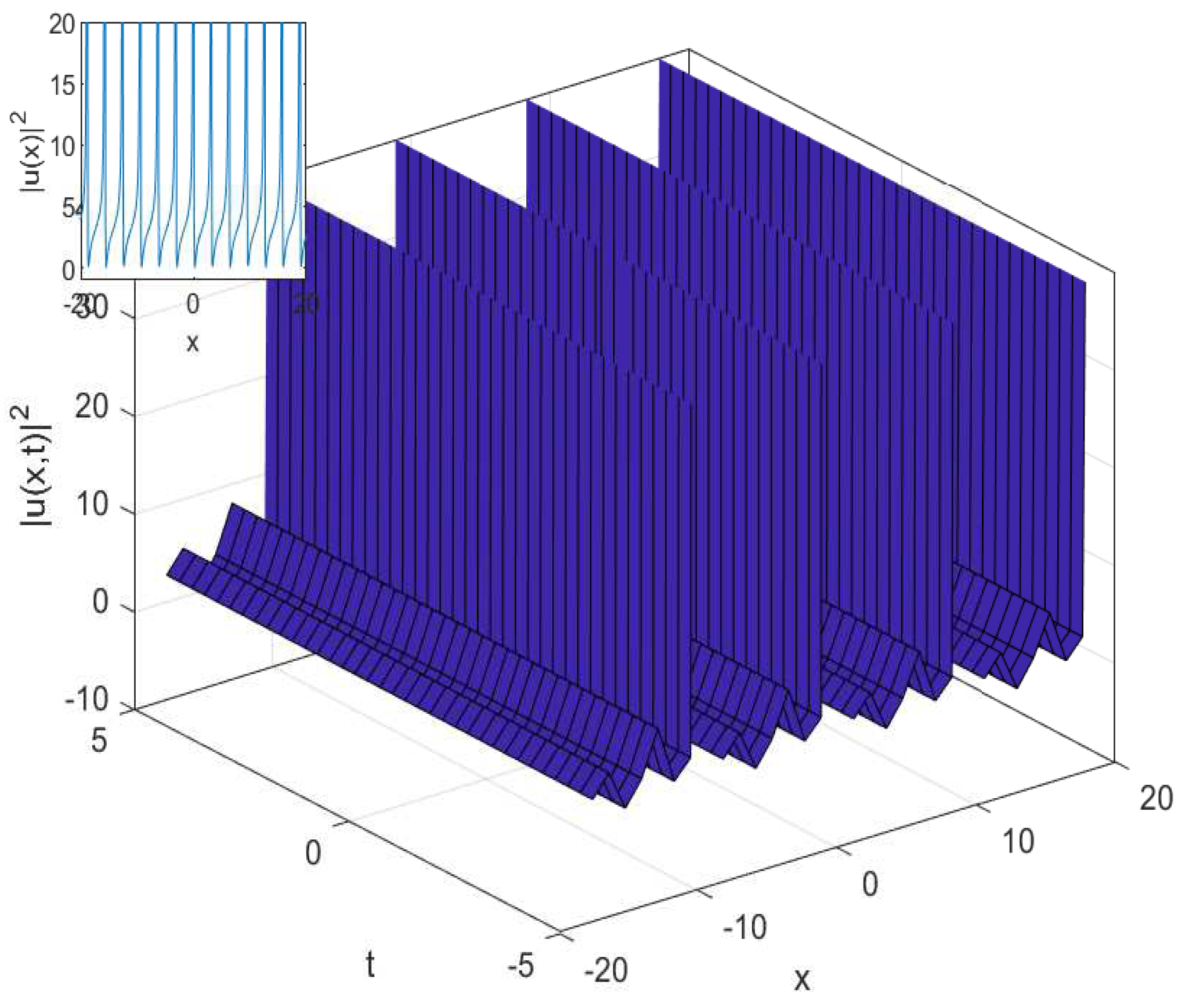
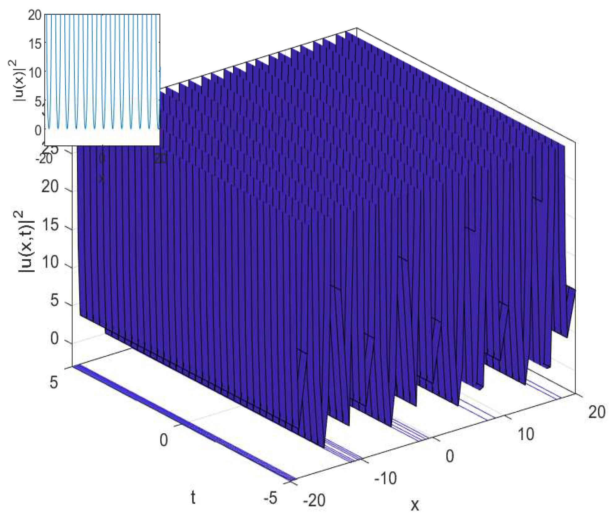
3.1. The Cubic-Quartic Nonlinear Schrödinger Equation

To solve Equation (3), by the $\left(m+\frac{G^{\prime }}{G}\right)$ expansion method, we use the following transformation:

$$u\left(x,t\right)=U\left(\xi \right)e^{{}^{i\theta }},\xi =x-\nu t,\theta =-\kappa x+\omega t.$$

(17)

In the above equation, $\theta \left(x,t\right)$ symbolize the phase component of the soliton, $\kappa$ represent the soliton frequency, while $\omega$ denote the wave number, and $\nu$ symbolize the velocity of the soliton. Substitute wave transformation into Equation (3), and separate the outcome equation into real and imaginary parts. We can write the real part as follows:

$$-\left(\alpha {\kappa }^3-\beta {\kappa }^4+\omega \right)U+c_1{U}^3+c_2{U}^5+3\alpha \kappa U^{″}-6\beta {\kappa }^2{U}^{″}+\beta U^{\left(4\right)}=0,$$

(18)

and the imaginary part can be written as:

$$\left(3\alpha {\kappa }^2-4\beta {\kappa }^3+\nu \right)U^{\prime }-\left(\alpha -4\beta \kappa \right)U^{\left(3\right)}=0.$$

(19)

From Equation (19) $U^{\prime }\ne 0$ and $U^{‴}\ne 0$, then:

$$\nu =4\beta {\kappa }^3-3\alpha {\kappa }^2,\alpha =4\beta \kappa .$$

(20)

Hence, Equation (18) can be rewritten as:

$$\left(3\beta {\kappa }^4+\omega \right)U-c_1{U}^3-c_2{U}^5-12\beta {\kappa }^2{U}^{″}+6\beta {\kappa }^2{U}^{″}-\beta U^{\left(4\right)}=0.$$

(21)

Multiplying both sides of Equation (21) by $U^{\prime }$ and taking its integration with respect to $\xi$, we get:

$$\beta \left(-12{\left(U^{″}\right)}^2+24U^{‴}{U}^{\prime }\right)+6c_1{U}^4+4c_2{U}^6+72\beta {\kappa }^2{\left(U^{\prime }\right)}^2-\left(36\beta {\kappa }^4+12\omega \right)U^2=0.$$

(22)

Finding the balance, we gain $n=1.$ Replacing this value of balance into Equation (8), we get:

$$U\left(\xi \right)=a_{-1}{\left(m+F\right)}^{-1}+a_0+a_1\left(m+F\right).$$

(23)

By substituting Equation (23) into Equation (3) by using Equation (9), we get the following solutions:

Case 1. When $a_0=\frac{\lambda a_1}{2},\kappa =\mp \frac{\sqrt{{\left(2m+\lambda \right)}^2-4\mu }}{\sqrt{6}},c_1=\frac{8\beta \left({\left(2m+\lambda \right)}^2-4\mu \right)}{a_1^2},c_2=-\frac{24\beta }{a_1^4},a_{-1}=0$, and $\Delta ={\left(\lambda +2m\right)}^2-4\mu$, we get an exponential function solution as follows:

$$\begin{array}{ll}u\left(x,t\right)=\hfill & {\mathrm{e}}^{\mathrm{i}\left(\sqrt{\frac{\Delta }{6}}x+\frac{5}{12}\beta {\Delta }^{2}t\right)}\\ & \left(\frac{\lambda a_1}{2}+a_1\left(m+\frac{1}{2}\left(-2m+\left(1-\frac{2A_1}{A_1+A_2{\mathrm{e}}^{\sqrt{\Delta }\left(x-\frac{2}{3}\sqrt{\frac{2}{3}}\beta {\left(\Delta \right)}^{3/2}t\right)}}\right)\sqrt{\Delta }-\lambda \right)\right)\right),\hfill \end{array}$$

(24)

which is a dark solution, as shown in Figure 1, $A_1\mathrm{and}{A}_2$ are non-zero numbers, and $\Delta >0$. Figure 1 shows that Equation (24) is a dark soliton under the suitable values of parameters.

Case 2. When $a_0=-\frac{\lambda a_{-1}}{2m\left(m+\lambda \right)-2\mu },a_1=0,a_2=\frac{12\omega }{5{\left({\left(2m+\lambda \right)}^2-4\mu \right)}^2},\kappa =\frac{\sqrt{{\left(2m+\lambda \right)}^2-4\mu }}{\sqrt{6}},c_1=\frac{96{\left(-m\left(m+\lambda \right)+\mu \right)}^2\omega }{5\left({\left(2m+\lambda \right)}^2-4\mu \right)a_{-1}^2},c_2=-\frac{288{\left(-m\left(m+\lambda \right)+\mu \right)}^4\omega }{5{\left({\left(2m+\lambda \right)}^2-4\mu \right)}^2{a}_{-1}^4},$ and $\Delta ={\left(\lambda +2m\right)}^2-4\mu$, we obtain an exponential function solution:

$$u\left(x,t\right)=\frac{a_{-1}{\mathrm{e}}^{\mathrm{i}\left(-\frac{x\sqrt{{\left(2m+\lambda \right)}^2-4\mu }}{\sqrt{6}}+t\omega \right)}}{m+\frac{1}{2}\left(-2m+\left(1-\frac{2A_1}{A_1+A_2{\mathrm{e}}^{\sqrt{\Delta }\left(x+\frac{8\sqrt{\frac{2}{3}}\omega }{5\sqrt{\Delta }}T\right)}}\right)\sqrt{\Delta }-\lambda \right)}+\frac{\lambda a_{-1}{\mathrm{e}}^{\mathrm{i}\left(-\frac{x\sqrt{{\left(2m+\lambda \right)}^2-4\mu }}{\sqrt{6}}+t\omega \right)}}{2m\left(m+\lambda \right)-2\mu },$$

(25)

which is a soliton solution, as shown in Figure 2, $A_1\mathrm{and}{A}_2$ are non-zero numbers, and $\Delta >0$.

With the suitable values, Figure 2 presents that Equation (25) is a singular soliton.

Case 3. When $a_{-1}=-\frac{\mathrm{i}\sqrt{3c_1}\left(m\left(m+\lambda \right)-\mu \right)}{\sqrt{c_2\left({\left(2m+\lambda \right)}^2-4\mu \right)}}$, $a_0=\frac{\mathrm{i}\sqrt{3c_1}\lambda }{2\sqrt{c_2\left({\left(2m+\lambda \right)}^2-4\mu \right)}}$, $a_1=0$, $\omega =-\frac{5{c_1}^2}{32c_2}$, $\kappa =\mp \frac{\sqrt{{\left(2m+\lambda \right)}^2-4\mu }}{\sqrt{6}}$, $\gamma =-\frac{3{c_1}^2}{8c_2{\left({\left(2m+\lambda \right)}^2-4\mu \right)}^2}$, and $\Delta ={\left(\lambda +2m\right)}^2-4\mu$, we have an exponential function solution:

$$\begin{array}{ll}\mathrm{u}\left(x,t\right)\hfill & ={\mathrm{e}}^{\mathrm{i}\left(-\frac{5c_1^2}{32c_2}t+\frac{\sqrt{\Delta }}{\sqrt{6}}x\right)}\\ & \left(\frac{\mathrm{i}\sqrt{3}\sqrt{c_1}\lambda }{2\sqrt{c_2\Delta }}-\frac{\mathrm{i}\sqrt{3}\sqrt{c_1}\left(m\left(m+\lambda \right)-\mu \right)}{\left(m+\frac{1}{2}\left(-2m+\left(1-\frac{2A_1}{A_1+A_2{\mathrm{e}}^{\sqrt{\Delta }\left(x+\frac{c_1^{2}t}{2\sqrt{6}{c}_2\sqrt{\Delta }}\right)}}\right)\sqrt{\Delta }-\lambda \right)\right)\sqrt{c_2\Delta }}\right),\hfill \end{array}$$

(26)

which is a soliton solution, as shown in Figure 3, $A_1\mathrm{and}{A}_2$ are non-zero numbers, and $\Delta >0$. Considering some values of parameters, Figure 3 shows singular soliton solution.

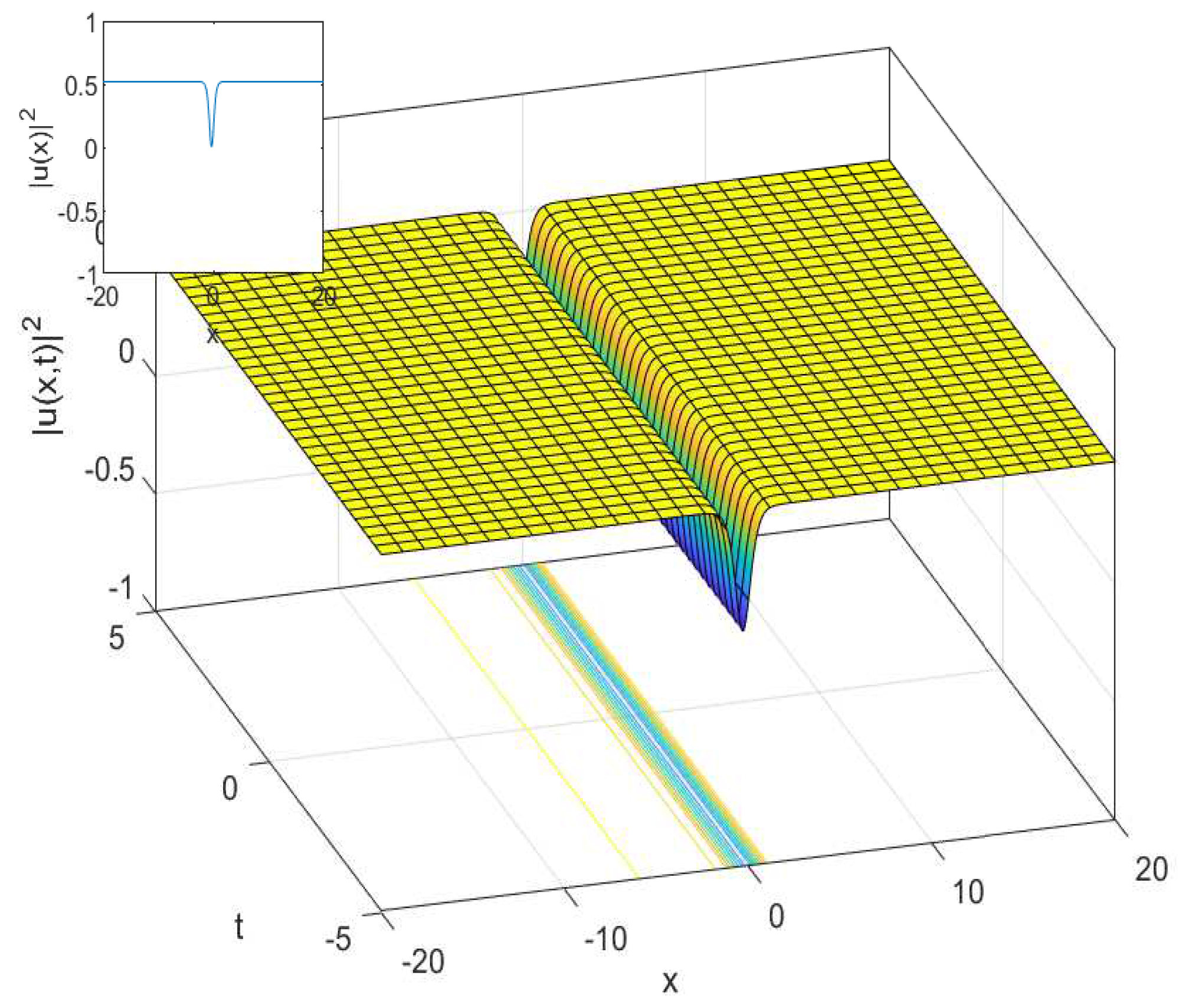
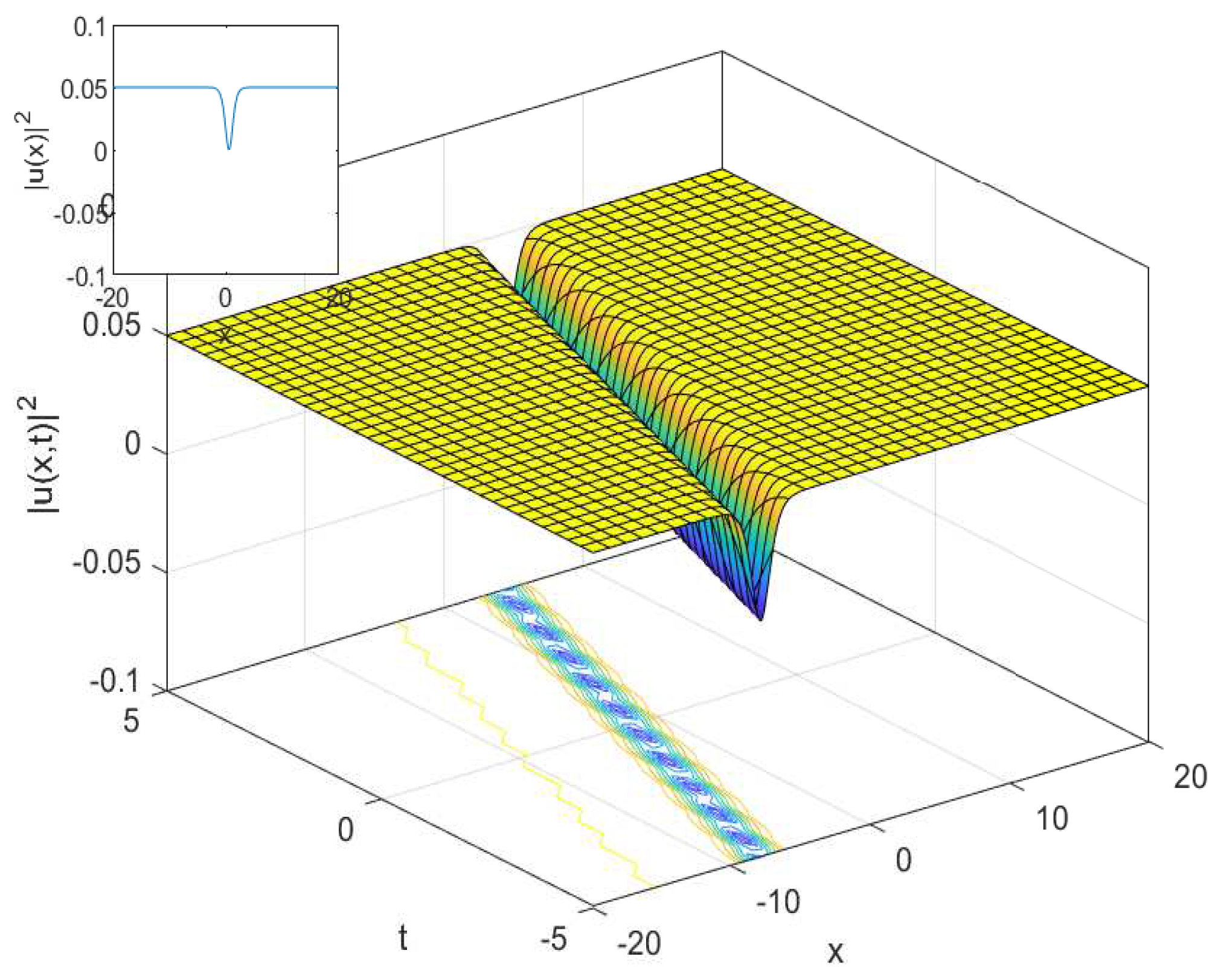
3.2. The Cubic-Quartic Resonant Nonlinear Schrödinger Equation

To solve Equation (4), by the $\left(m+\frac{G^{\prime }}{G}\right)$ expansion method, we consider wave transformation Equation (17). Replacing Equation (17) into Equation (4) and separating the outcome equation into real and imaginary parts, we can write the real part as follows:

$$\left({\kappa }^3\left(\alpha -\beta \kappa \right)+\omega \right)U-c_1{U}^3-c_2{U}^5-\left(c_3+3\kappa \left(\alpha -2\beta \kappa \right)\right)U^{″}-\beta U^{\left(4\right)}=0,$$

(27)

and the imaginary part can be written as:

$$\left(3\alpha {\kappa }^2-4\beta {\kappa }^3+\nu \right)U^{\prime }-\left(\alpha -4\beta \kappa \right)U^{‴}=0.$$

(28)

From Equation (28) $U^{\prime }\ne 0$ and $U^{‴}\ne 0$, then:

$$\nu =4\beta {\kappa }^3-3\alpha {\kappa }^2,\alpha =4\beta \kappa .$$

(29)

Hence, Equation (27) can be rewritten as:

$$\left(3\beta {\kappa }^4+\omega \right)U-c_1{U}^3-c_2{U}^5-\left(c_3+6\beta {\kappa }^2\right)U^{″}-\beta U^{\left(4\right)}=0.$$

(30)

Multiplying both sides of Equation (30) by $U^{\prime }$ and integrating it once with respect to $\xi$, we get:

$$\left(36\beta {\kappa }^4+12\omega \right)U^2-6c_1{U}^4-4c_2{U}^6-\left(12c_3+72\beta {\kappa }^2\right){\left(U^{\prime }\right)}^2+\beta \left(12{\left(U^{″}\right)}^2-24U^{\prime }{U}^{‴}\right)=0.$$

(31)

Finding the balance, we gain $n=1$. Putting this value into Equation (8), we get the same result of Equation (23). Substituting Equation (23) with Equation (9) into Equation (4), we get the following solutions:

Case 1. When $a_{-1}=-\frac{2\left(m\left(m+\lambda \right)-\mu \right)a_0}{\lambda }$, $a_1=0$, $\omega =\frac{1}{2}\beta \left(-6{\kappa }^4+{\left({\left(2m+\lambda \right)}^2-4\mu \right)}^2\right)$, $c_1=\frac{2\beta {\lambda }^2\left({\left(2m+\lambda \right)}^2-4\mu \right)}{a_0^2}$, $c_2=-\frac{3\beta {\lambda }^4}{2a_0^4}$, and $c_3=\beta \left(-6{\kappa }^2+{\left(2m+\lambda \right)}^2-4\mu \right)$, we obtain the following solutions:

Solution 1. In the case $\Delta >0$, we have an exponential function solution:

$$\begin{array}{ll}\mathrm{u}\left(x,t\right)\hfill & ={\mathrm{e}}^{\mathrm{i}\left(-\kappa x+\frac{1}{2}\beta \left(-6{\kappa }^4+{\left({\left(2m+\lambda \right)}^2-4\mu \right)}^2\right)t\right)}\\ & \left(a_0-\frac{2\left(m\left(m+\lambda \right)-\mu \right)a_0}{\left(m+\frac{1}{2}\left(-2m+\left(1-\frac{2A_1}{A_1+A_2{\mathrm{e}}^{\sqrt{\Delta }\left(x+8\beta {\kappa }^{3}t\right)}}\right)\sqrt{\Delta }-\lambda \right)\right)\lambda }\right).\hfill \end{array}$$

(32)

Considering some values of parameters, Figure 4 shows singular soliton solution.

Solution 2. In the case $\Delta <0$, we have a trigonometric function solution:

$$\begin{array}{ll}\mathrm{u}\left(x,t\right)\hfill & ={\mathrm{e}}^{-\mathrm{i}\kappa x+\frac{1}{2}\mathrm{i}\beta \left(-6{\kappa }^4+{\left({\left(2m+\lambda \right)}^2-4\mu \right)}^{2}t\right)}\\ & \left(a_0+\frac{4a_0\left(m^2+m\lambda -\mu \right)\left(A_2\cos \left(\alpha \right)+A_1\sin \left(\alpha \right)\right)}{\lambda \left(\left(-A_1\sqrt{-\Delta }+A_2\lambda \right)\cos \left(\alpha \right)+\left(A_2\sqrt{-\Delta }+A_1\lambda \right)\sin \left(\alpha \right)\right)}\right),\hfill \end{array}$$

(33)

which is $\alpha =\frac{1}{2}\sqrt{-\Delta }\left(x+8\beta {\kappa }^{3}t\right)$.

Periodic singular solution is plotted in Figure 5.

Case 2. When $a_{-1}=0$, $a_1=\frac{2a_0}{\lambda }$, $\omega =\frac{1}{2}\beta \left(-6{\kappa }^4+{\left({\left(2m+\lambda \right)}^2-4\mu \right)}^2\right)$, $c_1=\frac{2\beta {\lambda }^2\left({\left(2m+\lambda \right)}^2-4\mu \right)}{a_0^2}$, $c_2=-\frac{3\beta {\lambda }^4}{2a_0^4}$, and $c_3=\beta \left(-6{\kappa }^2+{\left(2m+\lambda \right)}^2-4\mu \right)$, we obtain the following solutions:

Solution 1. In the case $\Delta >0$, we get dark solution, as shown in Figure 6:

$$\begin{array}{ll}\mathrm{u}\left(x,y\right)\hfill & ={\mathrm{e}}^{\mathrm{i}\left(-\kappa x+\frac{1}{2}\beta \left(-6{\kappa }^4+{\left({\left(2m+\lambda \right)}^2-4\mu \right)}^2\right)t\right)}\\ & \left(a_0+\frac{2\left(m+\frac{1}{2}\left(-2m+\left(1-\frac{2A_1}{A_1+A_2{\mathrm{e}}^{\sqrt{\Delta }\left(x+8\beta {\kappa }^{3}t\right)}}\right)\sqrt{\Delta }-\lambda \right)\right)a_0}{\lambda }\right).\hfill \end{array}$$

(34)

Figure 6 shows the dark structure this solution.

Solution 2. In the case $\Delta <0$, we have a trigonometric function solution:

$$\begin{array}{ll}\mathrm{u}\left(x,t\right)\hfill & ={\mathrm{e}}^{-\mathrm{i}x\kappa +\frac{1}{2}\mathrm{i}\beta \left(-6{\kappa }^4+{\left({\left(2m+\lambda \right)}^2-4\mu \right)}^2\right)}t\\ & \left(\frac{\sqrt{-\Delta }\left(A_1\cos \left(\frac{1}{2}\sqrt{-\Delta }\left(x+8\beta {\kappa }^{3}t\right)\right)-A_2{a}_0\sin \left(\frac{1}{2}\sqrt{-\Delta }\left(x+8\beta {\kappa }^{3}t\right)\right)\right)}{\lambda \left(A_2\cos \left(\frac{1}{2}\sqrt{-\Delta }\left(x+8\beta {\kappa }^{3}t\right)\right)+A_1\sin \left(\frac{1}{2}\sqrt{-\Delta }\left(x+8\beta {\kappa }^{3}t\right)\right)\right)}\right).\hfill \end{array}$$

(35)

Periodic singular solution is plotted in Figure 7.

4. Application to the $\mathrm{Exp}\left(-\phi \left(\xi \right)\right)$ Expansion Method

In this section, we apply the exp$\left(-\phi \left(\xi \right)\right)$ expansion method to the cubic-quartic nonlinear Schrödinger and resonant nonlinear Schrödinger equations.

4.1. The Cubic-Quartic Nonlinear Schrödinger Equation

To apply this method on the cubic-quartic nonlinear Schrödinger equation, Equation (3), we utilize the same wave transformation of Equation (17). As a result, we get Equation (22). Finding the balance, we gain $n=1.$ By inserting the value of the balance into Equation (10), we get:

$$U\left(\xi \right)=b_0+b_1{e}^{-\phi \left(\xi \right)}.$$

(36)

Substituting Equation (40) into Equation (22) and setting each summation of the coefficients of the exponential identities of the same power to be zero, we discuss the following cases of the solutions.

Case 1. When $b_0=\frac{\lambda b_1}{2},c_1=\frac{8a_2\left({\lambda }^2-4\mu \right)}{b_1^2},c_2=-\frac{24a_2}{b_1^4},\kappa =-\frac{\sqrt{{\lambda }^2-4\mu }}{\sqrt{6}}$, and $\omega =\frac{5}{12}{a}_2{\left({\lambda }^2-4\mu \right)}^2$, we get the following solutions:

Solution 1. In the case ${\lambda }^2-4\mu >0$ and $\mu \ne 0$, we have a hyperbolic function solution:

$$\begin{array}{ll}u\left(x,t\right)\hfill & ={\mathrm{e}}^{\mathrm{i}\left(\frac{\sqrt{{\lambda }^2-4\mu }}{\sqrt{6}}x+\frac{5}{12}{a}_2{\left({\lambda }^2-4\mu \right)}^{2}t\right)}\\ & \left(\frac{\lambda b_1}{2}+\frac{2\mu b_1}{-\lambda -\sqrt{{\lambda }^2-4\mu }\tanh \left[\frac{1}{2}\left(c+x-\frac{2}{3}\sqrt{\frac{2}{3}}{a}_2{\left({\lambda }^2-4\mu \right)}^{3/2}t\right)\sqrt{{\lambda }^2-4\mu }\right]}\right).\hfill \end{array}$$

(37)

This is a dark soliton solution, as shown in Figure 8.

Solution 2. When ${\lambda }^2-4\mu >0$, $\mu =0$, and $\lambda \ne 0$, we have hyperbolic function solutions:

$$\begin{array}{ll}\mathrm{u}\left(x,t\right)\hfill & ={\mathrm{e}}^{\mathrm{i}\left(\frac{5}{12}\beta {\lambda }^{4}t+\frac{\sqrt{{\lambda }^2}}{\sqrt{6}}x\right)}\\ & \left(\frac{\lambda b_1}{2}+\frac{\lambda b_1}{-1+\cosh \left(\lambda \left(c+x-\frac{2}{3}\sqrt{\frac{2}{3}}\beta {\left({\lambda }^2\right)}^{3/2}t\right)\right)+\sinh \left(\lambda \left(c+x-\frac{2}{3}\sqrt{\frac{2}{3}}\beta {\left({\lambda }^2\right)}^{3/2}t\right)\right)}\right).\hfill \end{array}$$

(38)

This is a bright singular combo soliton solution, as shown in Figure 9.

Case 2. When $b_0=\frac{\sqrt{3}\sqrt{c_1}\lambda }{2\sqrt{-c_2\left({\lambda }^2-4\mu \right)}}$, $b_1=\frac{\sqrt{3}\sqrt{c_1}}{\sqrt{-c_2\left({\lambda }^2-4\mu \right)}}$, $\kappa =-\frac{\sqrt{{\lambda }^2-4\mu }}{\sqrt{6}}$, $\omega =-\frac{5{c_1}^2}{32c_2}$, and $\beta =-\frac{3c_1^2}{8c_2{\left({\lambda }^2-4\mu \right)}^2}$, we get the following solutions:

Solution 1. When ${\lambda }^2-4\mu >0$ and $\mu \ne 0$, we get a dark solution, as shown in Figure 10:

$$\begin{array}{ll}\mathrm{u}\left(x,t\right)\hfill & ={\mathrm{e}}^{\mathrm{i}\left(-\frac{5c_1^2}{32c_2}t+\frac{\sqrt{{\lambda }^2-4\mu }}{\sqrt{6}}x\right)}\\ \hfill & \left(\frac{\sqrt{3}\sqrt{c_1}\left({\lambda }^2-4\mu +\lambda \sqrt{{\lambda }^2-4\mu }\tanh \left(\frac{c_1^{2}t}{4\sqrt{6}{c}_2}+\frac{1}{2}\left(c+x\right)\sqrt{{\lambda }^2-4\mu }\right)\right)}{2\sqrt{-c_2\left({\lambda }^2-4\mu \right)}\left(\lambda +\sqrt{{\lambda }^2-4\mu }\tanh \left(\frac{c_1^{2}t}{4\sqrt{6}{c}_2}+\frac{1}{2}\left(c+x\right)\sqrt{{\lambda }^2-4\mu }\right)\right)}\right).\hfill \end{array}$$

(39)

Solution 2. When ${\lambda }^2-4\mu >0$ and $\mu =0$, we get hyperbolic function solution:

$$\mathrm{u}\left(x,t\right)={\mathrm{e}}^{\mathrm{i}\left(-\frac{5c_1^2}{32c_2}t+\frac{\sqrt{{\lambda }^2-4\mu }}{\sqrt{6}}x\right)}\left(\frac{\sqrt{3}\sqrt{c_1}\lambda \coth \left(\frac{1}{24}\lambda \left(12\left(c+x\right)+\frac{\sqrt{6}{c}_1^2}{c_2\sqrt{{\lambda }^2}}t\right)\right)}{2\sqrt{-c_2{\lambda }^2}}\right).$$

(40)

This is a singular soliton solution, as shown in Figure 11.

4.2. The Cubic-Quartic Resonant Nonlinear Schrödinger Equation

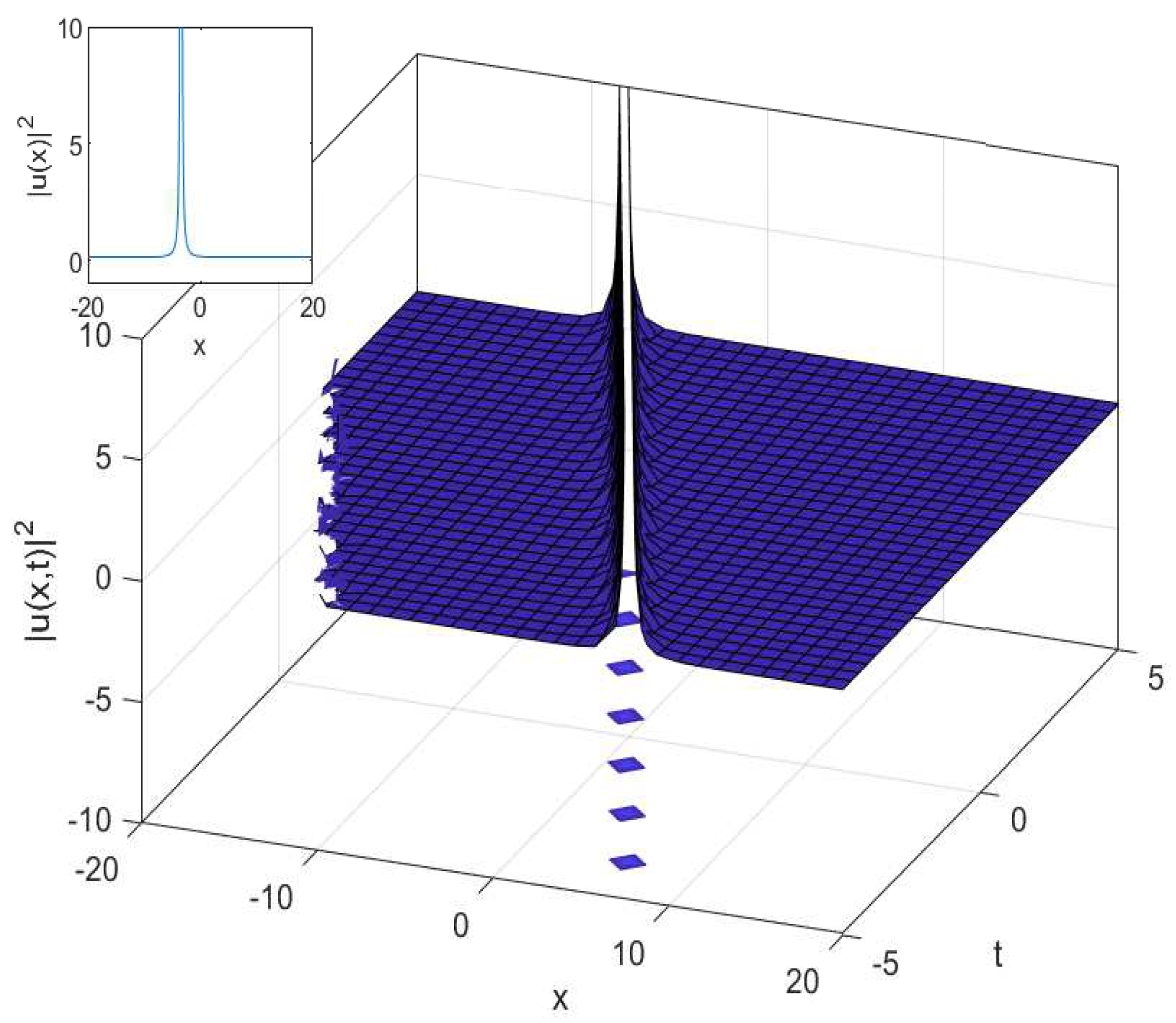
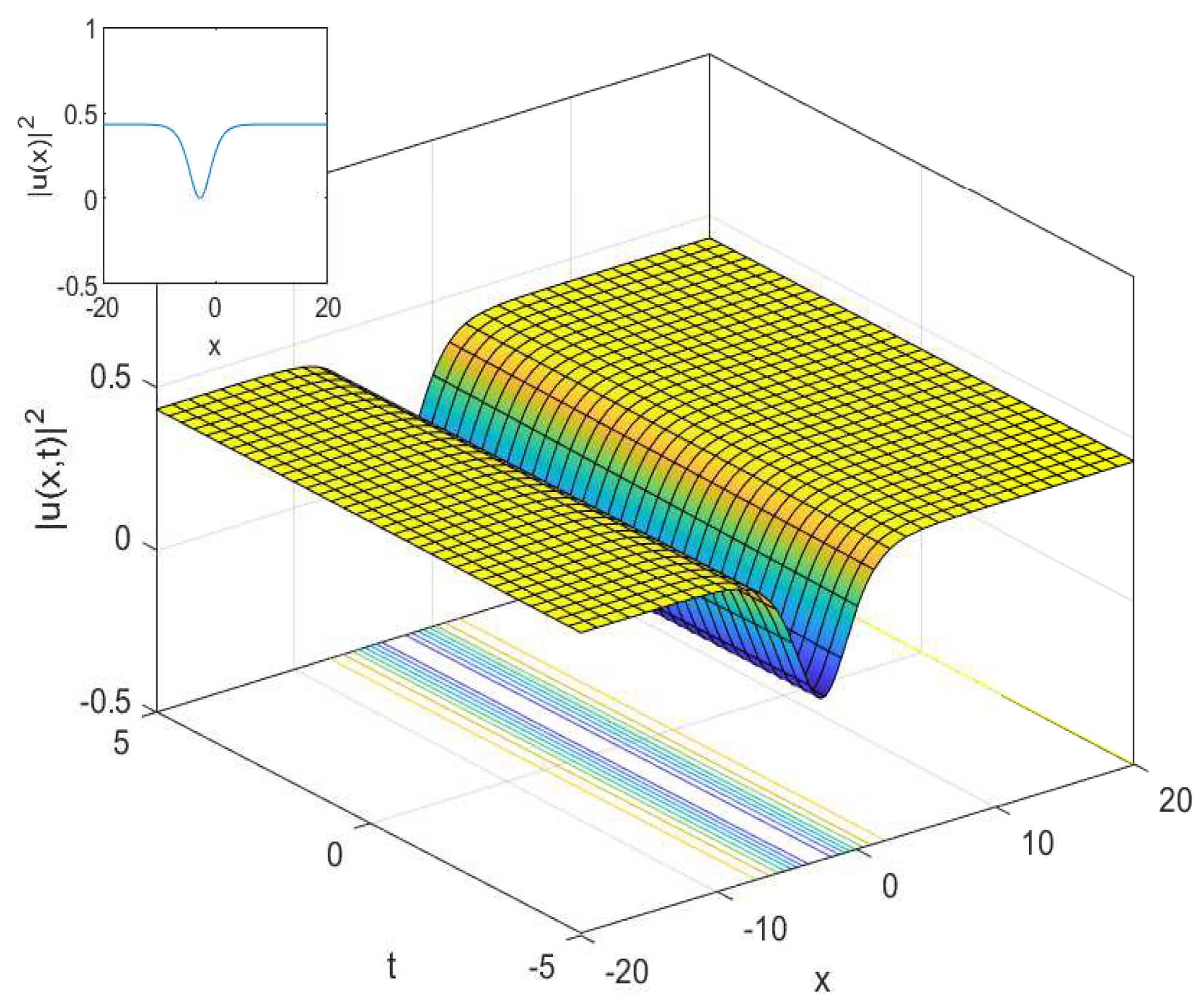
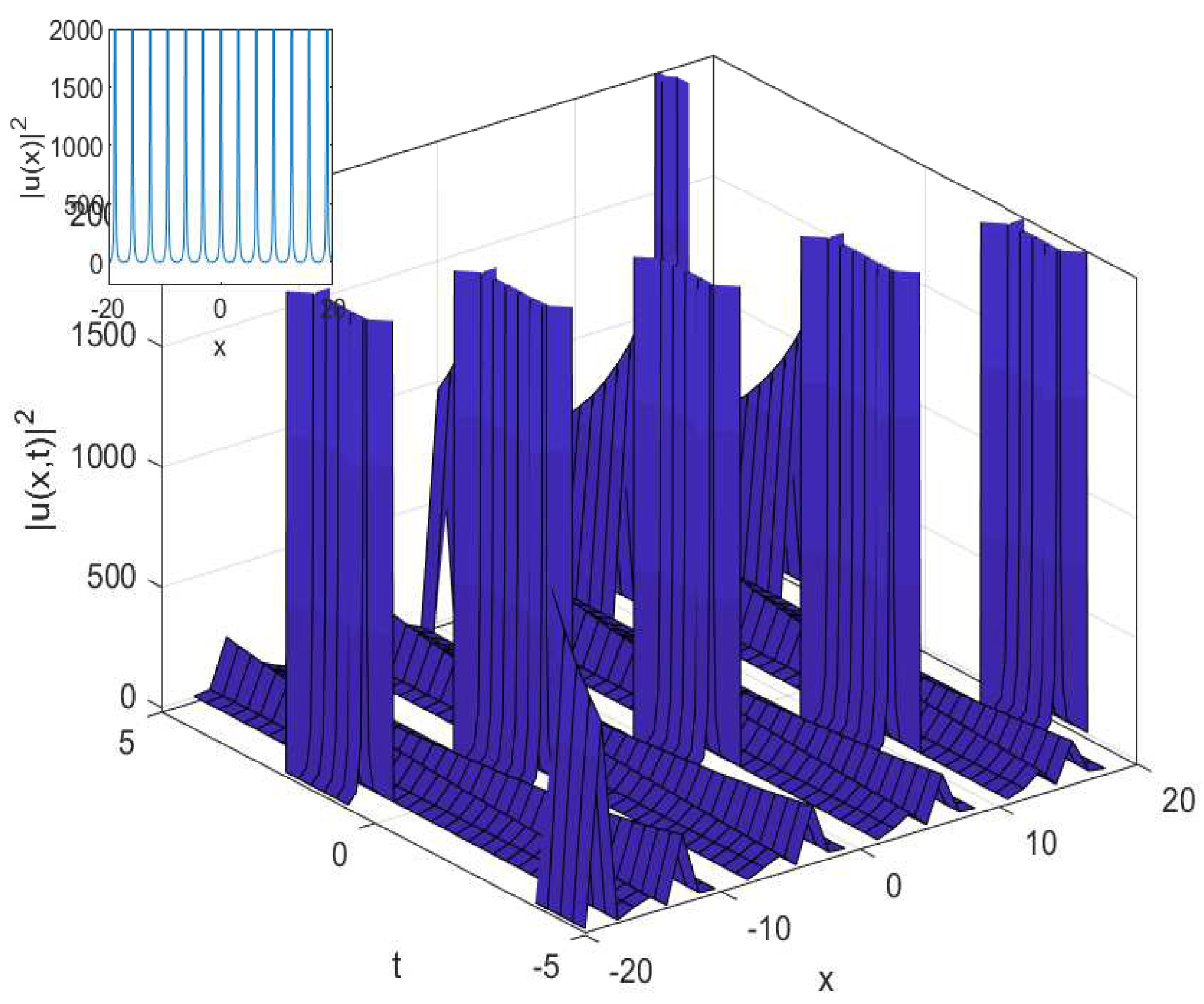
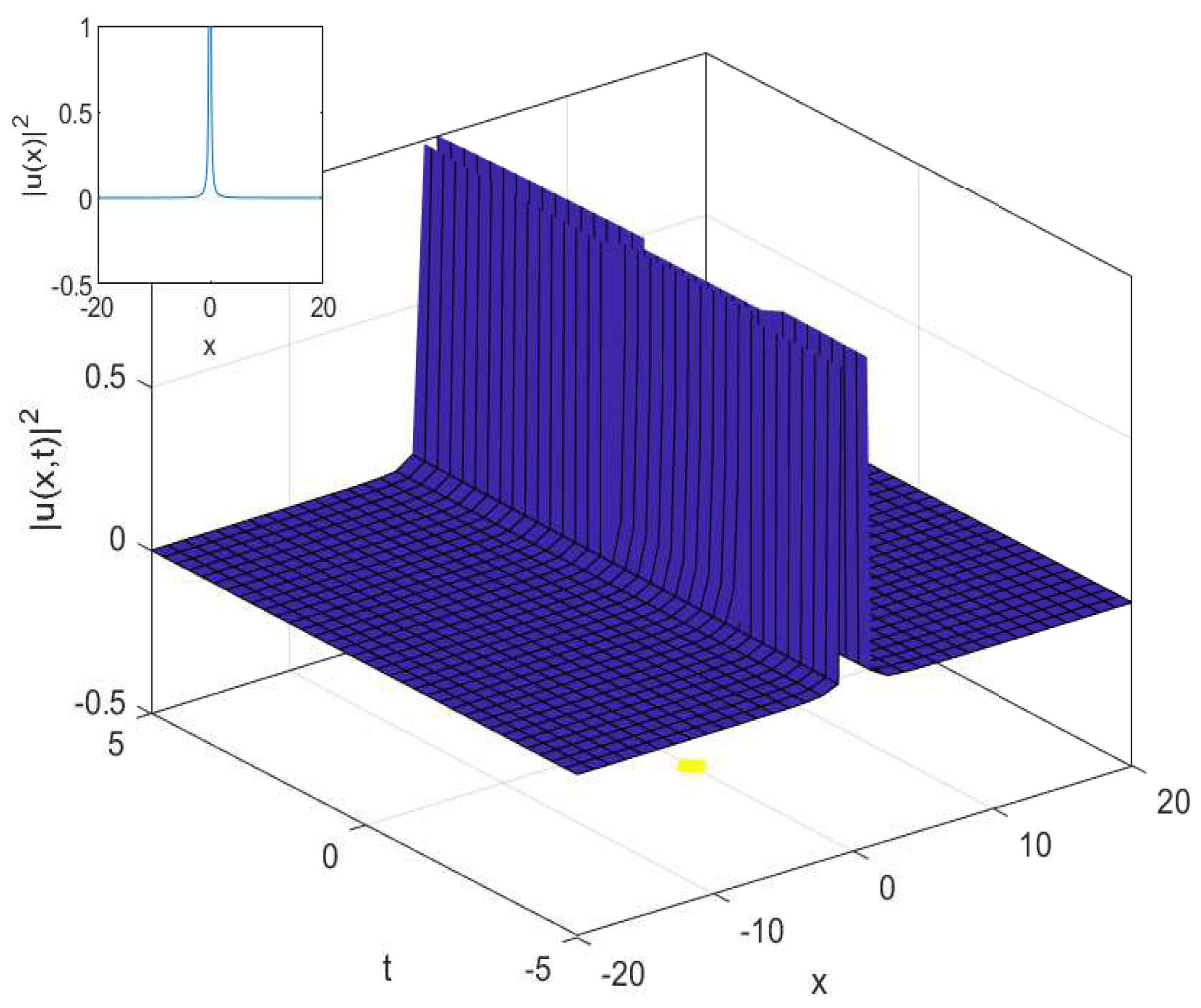
To apply the $\exp \left(-\phi \left(\xi \right)\right)$ expansion method on the cubic-quartic resonant nonlinear Schrödinger equation, Equation (4), we utilize the same wave transformation of Equation (17). As a result, we get Equation (31). Finding the balance, we gain $n=1.$ Via inserting the value of the balance into Equation (10), we get the same result of Equation (36). Substituting Equation (36) into Equation (31) and setting each summation of the coefficients of the exponential identities of the same power to be zero, we discuss the following cases of solutions.

Case 1. When $b_1=\frac{2b_0}{\lambda }$, $c_1=\frac{2\beta {\lambda }^2\left({\lambda }^2-4\mu \right)}{b_0^2}$, $c_2=-\frac{3\beta {\lambda }^4}{2b_0^4}$, $\kappa =\frac{\sqrt{-c_3+\beta \left({\lambda }^2-4\mu \right)}}{\sqrt{6}\sqrt{\beta }}$, and $\omega =\frac{-c{3}^2+2c3\beta \left({\lambda }^2-4\mu \right)+5{\beta }^2{\left({\lambda }^2-4\mu \right)}^2}{12\beta }$, we get the following solutions:

Solution 1. When ${\lambda }^2-4\mu >0$ and $\mu \ne 0$, we get hyperbolic function solution:

$$\begin{array}{ll}\mathrm{u}\left(x,t\right)\hfill & ={\mathrm{e}}^{\mathrm{i}\left(-\frac{\sqrt{-c_3+\beta \left({\lambda }^2-4\mu \right)}}{\sqrt{6}\sqrt{\beta }}x+\frac{\left(-c_3^2+2c_3\beta \left({\lambda }^2-4\mu \right)+5{\beta }^2{\left({\lambda }^2-4\mu \right)}^2\right)}{12\beta }t\right)}\\ \hfill & \left(b_0+\frac{4\mu b_0}{\lambda \left(-\lambda -\sqrt{{\lambda }^2-4\mu }\tanh \left[\frac{1}{2}\left(c+x+\frac{2\sqrt{\frac{2}{3}}t{\left(-c_3+\beta \left({\lambda }^2-4\mu \right)\right)}^{3/2}}{3\sqrt{\beta }}\right)\sqrt{{\lambda }^2-4\mu }\right]\right)}\right).\hfill \end{array}$$

(41)

This is a dark soliton solution, as shown in Figure 12.

Solution 2. When ${\lambda }^2-4\mu <0$ and $\mu \ne 0$, we get trigonometric function solution:

$$\begin{array}{ll}\mathrm{u}\left(x,t\right)\hfill & ={\mathrm{e}}^{\mathrm{i}\left(-\frac{x\sqrt{-c_3+\beta \left({\lambda }^2-4\mu \right)}}{\sqrt{6}\sqrt{\beta }}+\frac{t\left(-c_3^2+2c_3\beta \left({\lambda }^2-4\mu \right)+5{\beta }^2{\left({\lambda }^2-4\mu \right)}^2\right)}{12\beta }\right)}\\ \hfill & \left(b_0-\frac{4\mu b_0}{{\lambda }^2-\lambda \sqrt{-{\lambda }^2+4\mu }\tan \left[\frac{1}{2}\left(c+x+\frac{2\sqrt{\frac{2}{3}}{\left(-c_3+\beta \left({\lambda }^2-4\mu \right)\right)}^{3/2}}{3\sqrt{\beta }}t\right)\sqrt{-{\lambda }^2+4\mu }\right]}\right).\hfill \end{array}$$

(42)

This is a periodic singular soliton solution, as shown in Figure 13.

Solution 3. When ${\lambda }^2-4\mu >0$ and $\mu =0$, we get hyperbolic function solution:

$$\begin{array}{ll}\mathrm{u}\left(x,t\right)\hfill & ={\mathrm{e}}^{\mathrm{i}\left(-\frac{x\sqrt{-c_3+\beta {\lambda }^2}}{\sqrt{6}\sqrt{\beta }}+\frac{t\left(-c_3^2+2c_3\beta {\lambda }^2+5{\beta }^2{\lambda }^4\right)}{12\beta }\right)}\\ \hfill & \left(b_0+\frac{2b_0}{\cosh \left[\lambda \left(c+x+\frac{2\sqrt{\frac{2}{3}}t{\left(-c_3+\beta {\lambda }^2\right)}^{3/2}}{3\sqrt{\beta }}\right)\right]+\sinh \left[\lambda \left(c+x+\frac{2\sqrt{\frac{2}{3}}t{\left(-c_3+\beta {\lambda }^2\right)}^{3/2}}{3\sqrt{\beta }}\right)\right]}\right).\hfill \end{array}$$

(43)

This is a bright singular combo soliton solution, as shown in Figure 14.

Case 2. When $b_0=\frac{\sqrt{2}\sqrt{\beta {\lambda }^2\left({\lambda }^2-4\mu \right)}}{\sqrt{c1}}$, $b_1=\frac{2\sqrt{2}\sqrt{\beta {\lambda }^2\left({\lambda }^2-4\mu \right)}}{\sqrt{c_1}\lambda }$, $c_2=-\frac{3c_1^2}{8\beta {\left({\lambda }^2-4\mu \right)}^2}$, $c_3=\beta \left(-6{\kappa }^2+{\lambda }^2-4\mu \right)$, and $\omega =\frac{1}{2}\beta \left(-6{\kappa }^4+{\left({\lambda }^2-4\mu \right)}^2\right)$, we get the following solutions:

Solution 1. When ${\lambda }^2-4\mu >0$ and $\mu \ne 0$, we get hyperbolic function solution:

$$\begin{array}{ll}u\left(x,t\right)\hfill & =\sqrt{2\beta {\lambda }^2\left({\lambda }^2-4\mu \right)}{\mathrm{e}}^{-\mathrm{i}\kappa x+\frac{1}{2}\mathrm{i}\beta \left(-6{\kappa }^4+{\left({\lambda }^2-4\mu \right)}^2\right)t}\\ \hfill & \frac{\left(1-\frac{4\mu }{{\lambda }^2+\lambda \sqrt{{\lambda }^2-4\mu }\tanh \left[\frac{1}{2}\left(c+x+8\beta {\kappa }^{3}t\right)\sqrt{{\lambda }^2-4\mu }\right]}\right)}{\sqrt{c_1}}.\hfill \end{array}$$

(44)

This is a dark soliton solution, as shown in Figure 15.

Solution 2. When ${\lambda }^2-4\mu <0$ and $\mu \ne 0$, we get trigonometric function solution:

$$\begin{array}{ll}u\left(x,t\right)\hfill & =\sqrt{2\beta {\lambda }^2\left({\lambda }^2-4\mu \right)}{\mathrm{e}}^{-\mathrm{i}\kappa x+\frac{1}{2}\mathrm{i}\beta \left(-6{\kappa }^4+{\left({\lambda }^2-4\mu \right)}^2\right)t}\\ \hfill & \frac{\left(1-\frac{4\mu }{{\lambda }^2-\lambda \sqrt{-{\lambda }^2+4\mu }\tan \left[\frac{1}{2}\left(c+x+8t\beta {\kappa }^3\right)\sqrt{-{\lambda }^2+4\mu }\right]}\right)}{\sqrt{c_1}}.\hfill \end{array}$$

(45)

This is a periodic singular soliton solution, as shown in Figure 16.

Solution 3. When ${\lambda }^2-4\mu >0$ and $\mu =0$, we get the hyperbolic function solution:

$$u\left(x,t\right)=\frac{\sqrt{2}{\mathrm{e}}^{-\mathrm{i}\kappa x+\frac{1}{2}\mathrm{i}\beta \left(-6{\kappa }^4+{\lambda }^4\right)t}\sqrt{\beta {\lambda }^4}\coth \left(\frac{1}{2}\left(c+x+8\beta {\kappa }^{3}t\right)\lambda \right)}{\sqrt{c_1}},$$

(46)

which is a periodic singular solution, as shown in Figure 17.

5. Conclusions

In this research, the new dark, singular, bright singular combo soliton, and periodic singular solutions of the cubic-quantic nonlinear Schrödinger equation and the cubic-quantic resonant nonlinear Schrödinger equation were shown. Figure 1, Figure 6, Figure 8, Figure 10, Figure 12 and Figure 15 are dark soliton solutions, Figure 2, Figure 3 and Figure 4, Figure 11, Figure 14 and Figure 17 are singular soliton solutions, Figure 5, Figure 7, Figure 13 and Figure 16 are periodic singular solutions, and Figure 9 is bright singular combo soliton solution. The $\left(m+G^{\prime }/G\right)$ expansion and exp($-\phi \left(\xi \right)$) expansion methods were utilized to study these two models with the parabolic law. The new solutions verified the main equations after we substituted them into Equations (3) and (4) for the existence of the equation.

Conte and Musette introduced that wave transformation, which we considered in this paper, protects the Painleve conditions and its properties [48]. Therefore, it can be seen that all results verified their physical properties and presented their estimated wave behaviors. Therefore, one can observe that the wave transformation considered in this paper in Equation (17) satisfies these conditions. We substituted all solutions to the main equations Equations (3) and (4), and they verified it; the constraint conditions Equations (20) and (29) were also used to verify this existence. The optical soliton solutions obtained in this research paper may be of concern and useful in many fields of science, such as mathematical physics, applied physics, nonlinear science, and engineering.

References

1. Plastino, A. Entropic aspects of nonlinear partial differential equations: Classical and quantum mechanical perspectives. Entropy 2017, 19, 166. [Google Scholar] [CrossRef] [Green Version]
2. Ilhan, O.A.; Esen, A.; Bulut, H.; Baskonus, H.M. Singular solitons in the pseudo-parabolic model arising in nonlinear surface waves. Results Phys. 2019, 12, 1712–1715. [Google Scholar] [CrossRef]
3. Arshad, M.; Seadawy, A.R.; Lu, D. Exact bright–dark solitary wave solutions of the higher-order cubic–quintic nonlinear Schrödinger equation and its stability. Optik 2017, 138, 40–49. [Google Scholar] [CrossRef]
4. Arshad, M.; Seadawy, A.R.; Lu, D. Elliptic function and solitary wave solutions of the higher-order nonlinear Schrödinger dynamical equation with fourth-order dispersion and cubic-quintic nonlinearity and its stability. Eur. Phys. J. Plus 2017, 132, 371. [Google Scholar] [CrossRef]
5. Yousif, M.A.; Mahmood, B.A.; Ali, K.K.; Ismael, H.F. Numerical simulation using the homotopy perturbation method for a thin liquid film over an unsteady stretching sheet. Int. J. Pure Appl. Math. 2016, 107, 289–300. [Google Scholar] [CrossRef] [Green Version]
6. Baskonus, H.M.; Bulut, H. On the numerical solutions of some fractional ordinary differential equations by fractional Adams-Bashforth-Moulton method. Open Math. 2015, 13, 547–556. [Google Scholar] [CrossRef]
7. Ismael, H.F. Carreau-Casson fluids flow and heat transfer over stretching plate with internal heat source/sink and radiation. Int. J. Adv. Appl. Sci. 2017, 4, 11–15. [Google Scholar] [CrossRef]
8. Ali, K.K.; Ismael, H.F.; Mahmood, B.A.; Yousif, M.A. MHD Casson fluid with heat transfer in a liquid film over unsteady stretching plate. Int. J. Adv. Appl. Sci. 2017, 4, 55–58. [Google Scholar] [CrossRef]
9. Ismael, H.F.; Arifin, N.M. Flow and heat transfer in a maxwell liquid sheet over a stretching surface with thermal radiation and viscous dissipation. JP J. Heat Mass Transf. 2018, 15, 847–866. [Google Scholar] [CrossRef]
10. Zeeshan, A.; Ismael, H.F.; Yousif, M.A.; Mahmood, T.; Rahman, S.U. Simultaneous Effects of Slip and Wall Stretching/Shrinking on Radiative Flow of Magneto Nanofluid Through Porous Medium. J. Magn. 2018, 23, 491–498. [Google Scholar] [CrossRef]
11. Gao, W.; Partohaghighi, M.; Baskonus, H.M.; Ghavi, S. Regarding the group preserving scheme and method of line to the numerical simulations of Klein–Gordon model. Results Phys. 2019, 15, 102555. [Google Scholar] [CrossRef]
12. Yokus, A.; Baskonus, H.M.; Sulaiman, T.A.; Bulut, H. Numerical simulation and solutions of the two-component second order KdV evolutionarysystem. Numer. Methods Partial Differ. Equ. 2018, 34, 211–227. [Google Scholar] [CrossRef]
13. Sulaiman, T.A.; Bulut, H.; Yokus, A.; Baskonus, H.M. On the exact and numerical solutions to the coupled Boussinesq equation arising in ocean engineering. Indian J. Phys. 2019, 93, 647–656. [Google Scholar] [CrossRef]
14. Bulut, H.; Ergüt, M.; Asil, V.; Bokor, R.H. Numerical solution of a viscous incompressible flow problem through an orifice by Adomian decomposition method. Appl. Math. Comput. 2004, 153, 733–741. [Google Scholar] [CrossRef]
15. Ismael, H.F.; Ali, K.K. MHD casson flow over an unsteady stretching sheet. Adv. Appl. Fluid Mech. 2017, 20, 533–541. [Google Scholar] [CrossRef]
16. Baskonus, H.M.; Bulut, H.; Sulaiman, T.A. New Complex Hyperbolic Structures to the Lonngren-Wave Equation by Using Sine-Gordon Expansion Method. Appl. Math. Nonlinear Sci. 2019, 4, 141–150. [Google Scholar] [CrossRef] [Green Version]
17. Cattani, C.; Sulaiman, T.A.; Baskonus, H.M.; Bulut, H. On the soliton solutions to the Nizhnik-Novikov- Veselov and the Drinfel’d-Sokolov systems. Opt. Quantum Electron. 2018, 50, 138. [Google Scholar] [CrossRef]
18. Eskitaşçıoğlu, E.İ.; Aktaş, M.B.; Baskonus, H.M. New Complex and Hyperbolic Forms for Ablowitz–Kaup– Newell–Segur Wave Equation with Fourth Order. Appl. Math. Nonlinear Sci. 2019, 4, 105–112. [Google Scholar] [CrossRef] [Green Version]
19. Gao, W.; Ismael, F.H.; Bulut, H.; Baskonus, H.M. Instability modulation for the (2+1)-dimension paraxial wave equation and its new optical soliton solutions in Kerr media. Phys. Scr. 2019. [Google Scholar] [CrossRef]
20. Houwe, A.; Hammouch, Z.; Bienvenue, D.; Nestor, S.; Betchewe, G. Nonlinear Schrödingers equations with cubic nonlinearity: M-derivative soliton solutions by exp(-Φ(ξ))-Expansion method. Preprints 2019. [Google Scholar] [CrossRef]
21. Cattani, C.; Sulaiman, T.A.; Baskonus, H.M.; Bulut, H. Solitons in an inhomogeneous Murnaghan’s rod. Eur. Phys. J. Plus 2018, 133, 228. [Google Scholar] [CrossRef]
22. Baskonus, H.M.; Yel, G.; Bulut, H. Novel wave surfaces to the fractional Zakharov-Kuznetsov-Benjamin- Bona-Mahony equation. Proc. Aip Conf. Proc. 2017, 1863, 560084. [Google Scholar]
23. Baskonus, H.M.; Bulut, H. Exponential prototype structures for (2+1)-dimensional Boiti-Leon-Pempinelli systems in mathematical physics. Waves Random Complex Media 2016, 26, 189–196. [Google Scholar] [CrossRef]
24. Abdelrahman, M.A.E.; Sohaly, M.A. The Riccati-Bernoulli Sub-ODE Technique for Solving the Deterministic (Stochastic) Generalized-Zakharov System. Int. J. Math. Syst. Sci. 2018, 1. [Google Scholar] [CrossRef] [Green Version]
25. Gao, W.; Ismael, H.F.; Mohammed, S.A.; Baskonus, H.M.; Bulut, H. Complex and real optical soliton properties of the paraxial nonlinear Schrödinger equation in Kerr media with M-fractional. Front. Phys. 2019, 7, 197. [Google Scholar] [CrossRef] [Green Version]
26. Hammouch, Z.; Mekkaoui, T.; Agarwal, P. Optical solitons for the Calogero-Bogoyavlenskii-Schiff equation in (2 + 1) dimensions with time-fractional conformable derivative. Eur. Phys. J. Plus 2018, 133, 248. [Google Scholar] [CrossRef]
27. Manafian, J.; Aghdaei, M.F. Abundant soliton solutions for the coupled Schrödinger-Boussinesq system via an analytical method. Eur. Phys. J. Plus 2016, 131, 97. [Google Scholar] [CrossRef]
28. Guo, L.; Zhang, Y.; Xu, S.; Wu, Z.; He, J. The higher order rogue wave solutions of the Gerdjikov-Ivanov equation. Phys. Scr. 2014, 89, 035501. [Google Scholar] [CrossRef]
29. Ling, L.; Feng, B.F.; Zhu, Z. General soliton solutions to a coupled Fokas–Lenells equation. Nonlinear Anal. Real World Appl. 2018, 40, 185–214. [Google Scholar] [CrossRef] [Green Version]
30. Miah, M.M.; Ali, H.M.S.; Akbar, M.A.; Seadawy, A.R. New applications of the two variable G/G,1/G)-expansion method for closed form traveling wave solutions of integro-differential equations. J. Ocean Eng. Sci. 2019. [Google Scholar] [CrossRef]
31. Miah, M.M.; Ali, H.M.S.; Akbar, M.A.; Wazwaz, A.M. Some applications of the (G/G,1/G)-expansion method to find new exact solutions of NLEEs. Eur. Phys. J. Plus 2017, 132, 252. [Google Scholar] [CrossRef]
32. Yokuş, A. Comparison of Caputo and conformable derivatives for time-fractional Korteweg–de Vries equation via the finite difference method. Int. J. Mod. Phys. B 2018, 32, 1850365. [Google Scholar] [CrossRef]
33. Yokuş, A.; Kaya, D. Conservation laws and a new expansion method for sixth order Boussinesq equation. Proc. AIP Conf. Proc. 2015, 1676, 020062. [Google Scholar]
34. Yang, X.; Yang, Y.; Cattani, C.; Zhu, C.M. A new technique for solving the 1-D Burgers equation. Therm. Sci. 2017, 21, 129–136. [Google Scholar] [CrossRef] [Green Version]
35. Vakhnenko, V.O.; Parkes, E.J.; Morrison, A.J. A Bäcklund transformation and the inverse scattering transform method for the generalised Vakhnenko equation. Chaos Solitons Fractals 2003, 17, 683–692. [Google Scholar] [CrossRef]
36. Jawad, A.J.M.; Abu-AlShaeer, M.J.; Biswas, A.; Zhou, Q.; Moshokoa, S.; Belic, M. Optical solitons to Lakshmanan-Porsezian-Daniel model for three nonlinear forms. Optik 2018, 160, 197–202. [Google Scholar] [CrossRef]
37. Biswas, A.; Triki, H.; Zhou, Q.; Moshokoa, S.P.; Ullah, M.Z.; Belic, M. Cubic–quartic optical solitons in Kerr and power law media. Optik 2017, 144, 357–362. [Google Scholar] [CrossRef]
38. Xie, Y.; Yang, Z.; Li, L. New exact solutions to the high dispersive cubic–quintic nonlinear Schrödinger equation. Phys. Lett. Sect. A Gen. At. Solid State Phys. 2018, 382, 2506–2514. [Google Scholar] [CrossRef]
39. Li, H.M.; Xu, Y.S.; Lin, J. New optical solitons in high-order dispersive cubic-quintic nonlinear Schrödinger equation. Commun. Theor. Phys. 2004, 41, 829. [Google Scholar]
40. Nawaz, B.; Ali, K.; Abbas, S.O.; Rizvi, S.T.R.; Zhou, Q. Optical solitons for non-Kerr law nonlinear Schrödinger equation with third and fourth order dispersions. Chin. J. Phys. 2019, 60, 133–140. [Google Scholar] [CrossRef]
41. Biswas, A.; Arshed, S. Application of semi-inverse variational principle to cubic-quartic optical solitons with kerr and power law nonlinearity. Optik 2018, 172, 847–850. [Google Scholar] [CrossRef]
42. Seadawy, A.R.; Kumar, D.; Chakrabarty, A.K. Dispersive optical soliton solutions for the hyperbolic and cubic-quintic nonlinear Schrödinger equations via the extended sinh-Gordon equation expansion method. Eur. Phys. J. Plus 2018, 133, 182. [Google Scholar] [CrossRef]
43. El-Dessoky, M.M.; Islam, S. Chirped Solitons in Generalized Resonant Dispersive Nonlinear Schrödinger’s equation. Comput. Sci. 2019, 14, 737–752. [Google Scholar]
44. Bansal, A.; Biswas, A.; Zhou, Q.; Babatin, M.M. Lie symmetry analysis for cubic–quartic nonlinear Schrödinger’s equation. Optik 2018, 169, 12–15. [Google Scholar] [CrossRef]
45. Biswas, A.; Kara, A.H.; Ullah, M.Z.; Zhou, Q.; Triki, H.; Belic, M. Conservation laws for cubic–quartic optical solitons in Kerr and power law media. Optik 2017, 145, 650–654. [Google Scholar] [CrossRef]
46. Younis, M.; Cheemaa, N.; Mahmood, S.A.; Rizvi, S.T.R. On optical solitons: The chiral nonlinear Schrödinger equation with perturbation and Bohm potential. Opt. Quantum Electron. 2016, 48, 542. [Google Scholar] [CrossRef]
47. Hosseini, K.; Samadani, F.; Kumar, D.; Faridi, M. New optical solitons of cubic-quartic nonlinear Schrödinger equation. Optik 2018, 157, 1101–1105. [Google Scholar] [CrossRef]
48. Conte, R.; Musette, M. Elliptic general analytic solutions. Stud. Appl. Math. 2009, 123, 63–81. [Google Scholar] [CrossRef]
Figure 1. 3D surface of Equation (24), which is a dark optical soliton solution plotted when A 1 = 1 , A 2 = 0.3 , β = 0.2 , a 1 = 0.4 , λ = 1 , m = 1 , μ = 1 , and t = 2 for 2D.
Applsci 10 00219 g001
Figure 2. 3D surface of Equation (25), which is a singular soliton solution plotted when A 1 = 2 , A 2 = 3 , β = 6 , a 1 = 6 , λ = 1 , m = 1 , μ = 1 , and t = 2 for 2D.
Applsci 10 00219 g002
Figure 3. 3D surface of Equation (26), which is a singular soliton solution plotted when A 1 = 0.3 , A 2 = 2 , c 1 = 0.3 , c 2 = 2 , λ = 1 , m = 1 , μ = 1 , and t = 2 for 2D.
Applsci 10 00219 g003
Figure 4. 3D figure of Equation (32), which is a singular soliton solution plotted when A 1 = 1 , A 2 = 3 , λ = 1 , m = 1 , μ = 1 , β = 0.2 , a 0 = 0.2 , κ = 0.01 , and t = 2 for 2D.
Applsci 10 00219 g004
Figure 5. 3D surface of Equation (33), which is a periodic singular soliton solution plotted when A 1 = 1 , A 2 = 2 , λ = 1 , m = 1 2 , μ = 2 , β = 0.1 , a 0 = 2 , κ = 0.1 , and t = 2 for 2D.
Applsci 10 00219 g005
Figure 6. 3D surface of Equation (34), which is a dark soliton solution plotted when A 1 = 1 , A 2 = 3 , λ = 1 , m = 1 , μ = 1 , β = 0.2 , a 0 = 0.2 , κ = 0.01 , and t = 2 for 2D.
Applsci 10 00219 g006
Figure 7. 3D figure of Equation (35), which is a periodic singular soliton solution plotted when A 1 = 1 , A 2 = 2 , λ = 1 , m = 1 2 , μ = 2 , β = 0.1 , a 0 = 0.2 , κ = 0.1 , and t = 2 for 2D.
Applsci 10 00219 g007
Figure 8. 3D surface of Equation (37), which is a bright singular combo soliton solution plotted when b 1 = 0.2 , β = 0.2 , c = 1 , λ = 3 , μ = 1 , and t = 2 for 2D.
Applsci 10 00219 g008
Figure 9. 3D surface of Equation (38), which is a bright singular combo soliton solution plotted when b 1 = 0.04 , β = 0.2 , c = 0.2 , λ = 1 , μ = 0 , and t = 2 for 2D.
Applsci 10 00219 g009
Figure 10. 3D surface of Equation (39), which is a dark soliton solution plotted when b 1 = 0.2 , β = 0.2 , c 1 = 0.1 , c 2 = 0.1 , c = 1 , λ = 3 , μ = 1 , and t = 2 for 2D.
Applsci 10 00219 g010
Figure 11. 3D figure of Equation (40), which is a singular soliton solution plotted when b 1 = 4 , β = 0.2 , c 1 = 0.1 , c 2 = 0.1 , c = 0.2 , λ = 1 , μ = 0 , and t = 2 for 2D.
Applsci 10 00219 g011
Figure 12. 3D surface of Equation (41), which is a dark soliton solution plotted when b 0 = 0.2 , β = 0.2 , c 3 = 1 , c = 1 , λ = 3 , μ = 1 , and t = 2 for 2D.
Applsci 10 00219 g012
Figure 13. 3D surface of Equation (42), which is a periodic singular soliton solution plotted when b 0 = 0.4 , β = 0.1 , c 3 = 5 , c = 1 , λ = 1 , μ = 1 , and t = 2 for 2D.
Applsci 10 00219 g013
Figure 14. 3D surface of Equation (43), which is a singular soliton solution plotted when b 0 = 0.4 , β = 0.2 , c 3 = 1 , c = 0.2 , λ = 3 , μ = 0 , and t = 2 for 2D.
Applsci 10 00219 g014
Figure 15. 3D surface of Equation (44), which is a dark soliton solution plotted when β = 3 , c 1 = 5 , c = 0.03 , λ = 1 , μ = 0.1 , κ = 0.1 , and t = 2 for 2D.
Applsci 10 00219 g015
Figure 16. 3D surface of Equation (45), which is a periodic singular soliton solution plotted when β = 3 , c 1 = 5 , c = 0.03 , λ = 0.1 , μ = 1 , κ = 0.1 , and t = 2 for 2D.
Applsci 10 00219 g016
Figure 17. 3D surface of Equation (46), which is a singular soliton solution plotted when β = 3 , c 1 = 5 , c = 0.03 , λ = 0.1 , μ = 0 , κ = 0.1 , and t = 2 for 2D.
Applsci 10 00219 g017