1. Introduction
Data compression has long been an important topic in the field of signal processing. With the broad use of smartphone and tablet cameras, vast amounts of multimedia content, mostly images, have accumulated. Thus, how a mechanism for efficiently performing data compression on the multimedia contents is urgent. There have been successful and popular standards for image compression including the well-known JPEG, which employs discrete cosine transform (DCT), and JPEG2000, which applies discrete wavelet transform (DWT), to still images. With the evolution of new techniques, advancements in data compression can also be expected, and compressed sensing techniques present new and novel concepts.
Compressed sensing (CS) is one recently developed technique of lossy data compression research and applications [
1,
2,
3,
4]. In addition to international standards in multimedia compression, such as JPEG [
5] or JPEG2000 [
6], it would be constructive to explore new innovative compression techniques. The major research looking at JPEG, JPEG2000, and CS focuses on compression performance by balancing the amount of compressed data and the reconstructed quality. In CS, this requires a sampling rate that is far less than the Nyquist rate and has the ability to reconstruct the original signal of lossy compression. The primary goal in compressed sensing research is the compression capability. Therefore, a method for effectively decoding the extremely small amount of compressed signals and comparing this to counterparts in JPEG or JPEG2000 would be of great interest and is currently a major challenge [
7,
8,
9]. In this paper, in addition to looking at compression performance, we consider practical scenarios of robust transmission of compressed sensing signals using block compressed sensing (BCS) [
10,
11,
12]. We transmitted compressed signals over lossy channels to observe the effect of packet losses. To reduce quality degradation of robust transmission [
13,
14,
15], we employed the transmission of BCS signals over multiple independent channels. Multiple description coding (MDC) [
16,
17] was employed to protect and reconstruct the BCS signals. To better explore the performance of BCS, we used adaptive sampling [
18,
19]. This way, the enhanced quality of the reconstructed image can be observed for error controlled transmission. Therefore, the novelty of this paper is the error resilient transmission of BCS with MDC. We observed enhanced performance using our algorithm.
This paper is organized as follows. In
Section 2 we briefly describe the fundamentals and mathematical representations of BCS. In
Section 3 we present the proposed method for error resilient transmission of compressed sensing signals over multiple independent and lossy channels. The simulation results are demonstrated in
Section 4. Here we point out the vulnerability of compressively sensed signals transmitted over a single channel and how our algorithm for multiple-channel transmission for grey-level and color images reduced image quality degradation. Finally, we address the conclusion of this paper in
Section 5.
3. Proposed Algorithm
For the effective delivery of compressed sensing signals, and considering the robust transmission depicted in [
14], we employed the use of transmission over multiple mutually independent lossy channels.
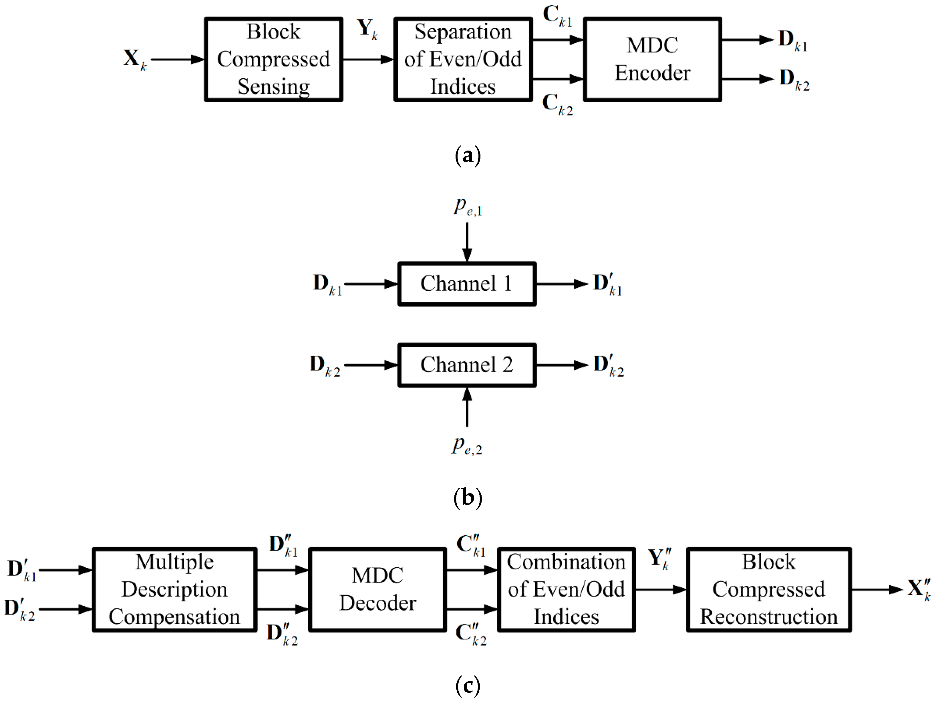
Figure 1 describes the block diagram of our system.
In
Figure 1a, the input image
is divided into
. It is then compressed with BCS and the compressed sensing signal is denoted by
. With the notations described in
Section 2, we denoted
and set
to an even number for application with multiple description coding. To enable easy separation of BCS coefficients, we chose the odd numbered indices to form
, and the even numbered ones to form
. For ease of representation, we rearranged the notations to be
and
After that, we employed multiple description transform coding (MDTC) [
15] in MDC to form the elements in the two descriptions of
and
in Equation (9):
where
. The 2 × 2 matrix in Equation (9) has the condition that
, leading to the determinant of one. The resulting elements in Equation (9) form the two descriptions
and
.
Next, descriptions
and
were transmitted over two independent lossy channels, with the loss probability of
and
for Channels 1 and 2, as depicted in
Figure 1b. The received descriptions may become
and
due to the possibility of induced errors. Note that
and
may not be identical to their counterparts
and
, respectively.
At the decoder, as shown in
Figure 1c by employing [
16], compensation should be applied between received descriptions. Compensated descriptions
and
was calculated first. The elements in the descriptions
and
,
were compensated as follows:
By taking the inverse operations of Equation (9), compensated BCS coefficients were obtained in Equation (12):
By gathering all the elements together,
and
were formed from the compensated descriptions in Equation (12). Here we denote
and
After the combination of the even and odd indexed components in Equations (13) and (14) and
Figure 1c, we obtained
. Finally, using BCS we reconstructed block
. After completing the reconstruction of all the blocks, we composed the reconstructed image
.
4. Simulation Results
In our simulations we provided three sets of experiments based on three test images. The first was cameraman grey-level test image with a size of 256 × 256. The second was the ducks color image, taken by the authors, with a size of 1024 × 1024. The third was the Pasadena-houses color image with a size of 1760 × 1168 [
22]. These three images were employed in the experiments.
Here we start the first set of experiments with the test image cameraman. In
Figure 2, we present the use of entropy for adaptive sampling. Considering the practical implementation of adaptive sampling, we applied quantization to the entropy values with a step size of 0.1.
Figure 2a presents the original test image, cameraman. The relationship between the number of blocks and entropy is depicted in
Figure 2b. Smaller entropy values imply smoother blocks.
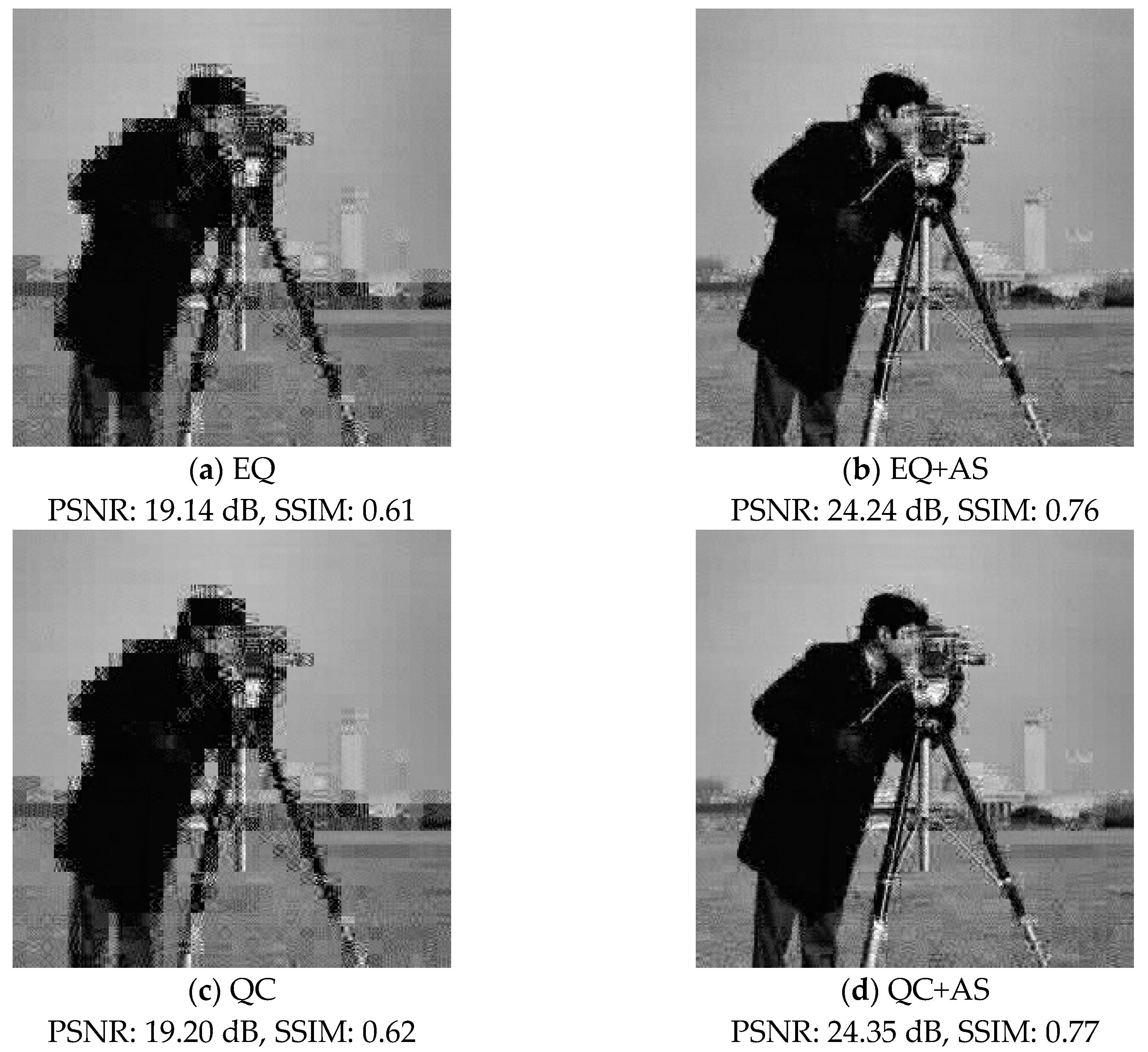
Figure 3 presents the error-free transmission of BCS for cameraman. Considering the practical applications, we chose
in BCS in Equation (1). The measurement rate was set to
, meaning that
compressed sensing coefficients were selected per block on the average. The reconstructed images were assessed with the peak signal-to-noise ratio (PSNR) and the structural similarity (SSIM) [
23].
Figure 3a shows only the reconstruction for equality constraint (EQ). Because adaptive sampling was not applied, it is implied that every block was reconstructed with 12 BCS coefficients.
Figure 3b presents the reconstruction for equality constraint (EQ) with adaptive sampling (AS) [
10]. Here we use the abbreviation EQ + AS for the results in
Figure 3b. Because adaptive sampling was applied, the number of BCS coefficients varied from one block to another. Blocks with larger entropies were designated a higher number of BCS coefficients, and vice versa. The average number of BCS coefficients for all the blocks was 12. Via adaptive sampling, we easily observed enhanced performances.
Figure 3c,d led to the results for quadratic constraint (QC) and quadratic constraint with adaptive sampling (QC + AS), respectively. Again, with adaptive sampling, better performances were observed. We also compared the results of
Figure 3a,c. With the quadratic constraint in Equation (4) it performed slightly better than its counterpart, equality constraint, in Equation (3). Similar phenomena can also be found by comparing
Figure 3b,d.
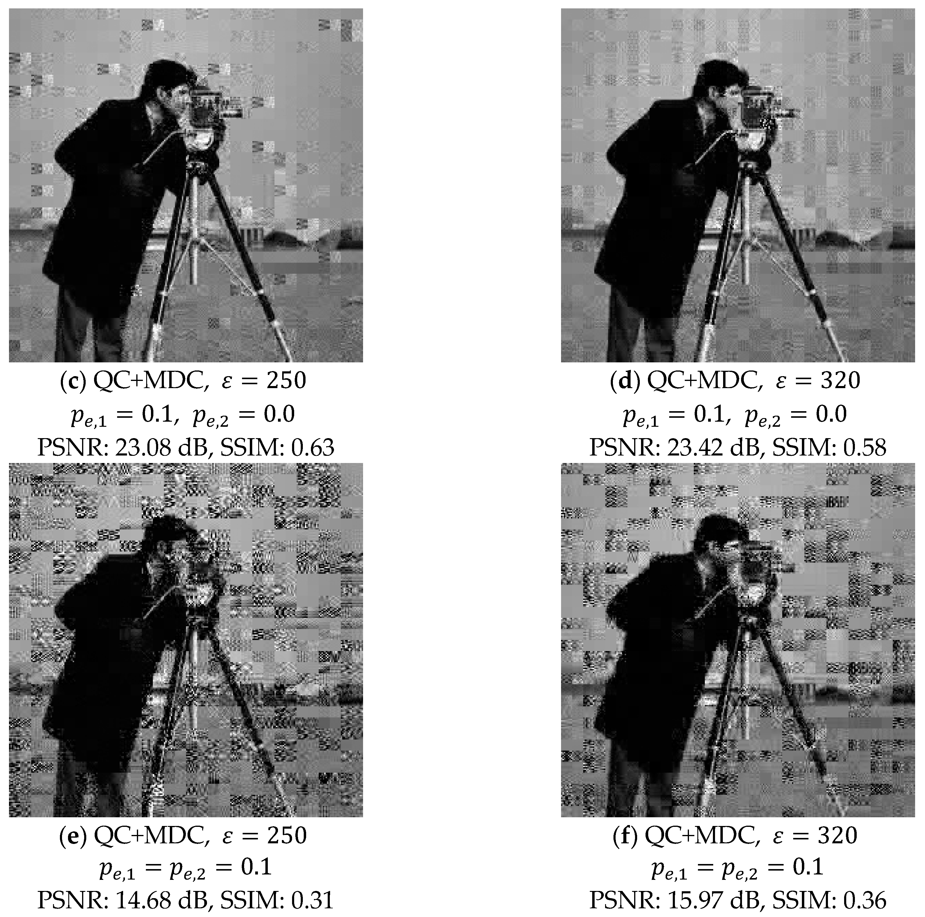
In
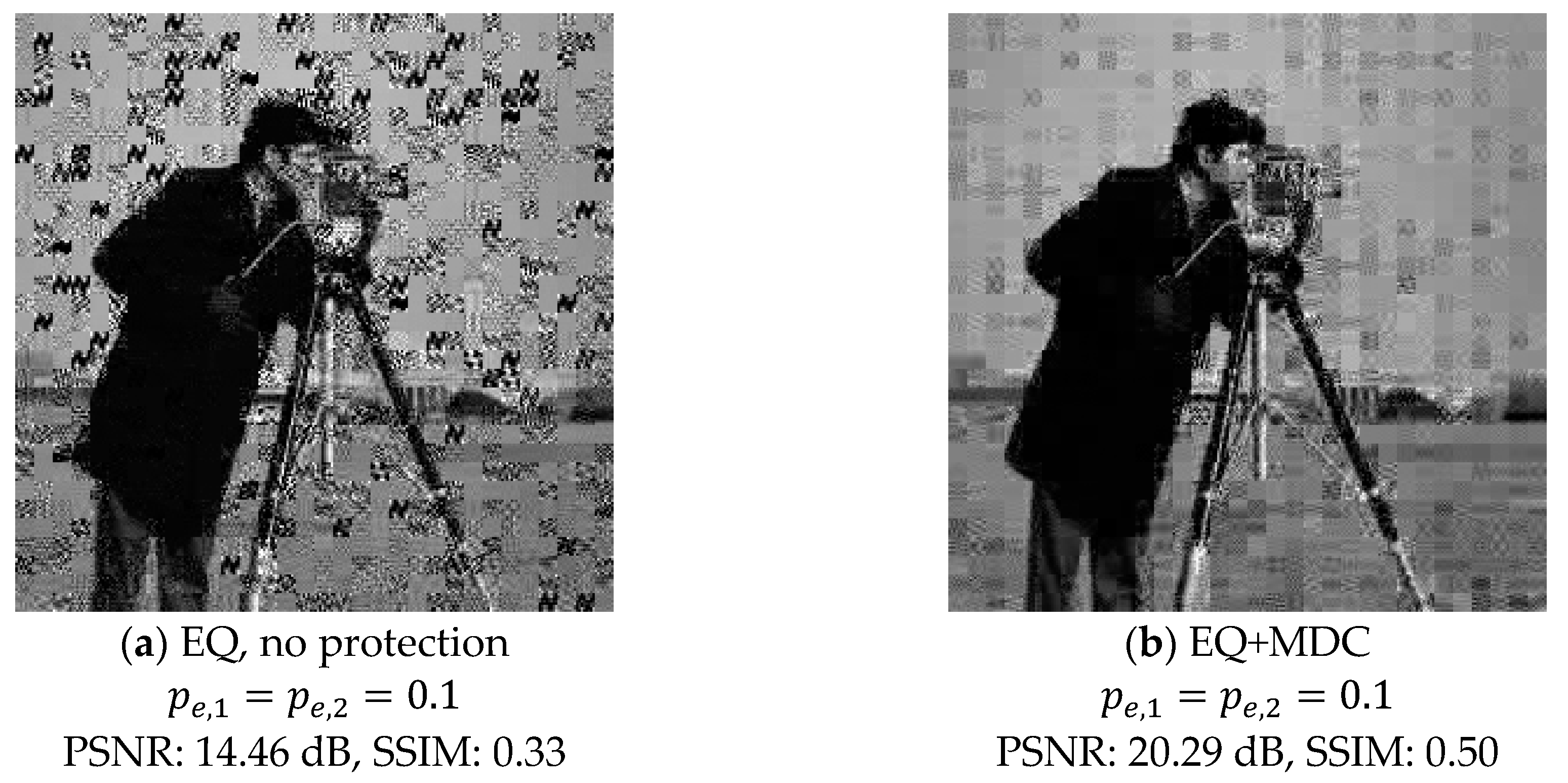
Figure 4 we present the lossy transmission for block compressed sensing with adaptive sampling. In
Figure 4a,b, when the BCS coefficients were transmitted over the two independent and lossy channels in
Figure 1b, we set
. Here we employed the equality constraint (EQ) for reconstruction. Constructing the received BCS coefficients directly led to the result in
Figure 4a, meaning that some protection may be required. In
Figure 4b, we applied multiple description coding from Equation (9) for protection. The parameters were chosen to be
,
, and
, and this led to
from calculations using Equation (9). With the compensation techniques of MDC from Equation (9), we observed that the reconstructed quality was greatly improved. In addition, for the evaluation of reconstruction under severely lost channels we set
, with the results shown in
Figure 4c,d. Severe degradation was easily visible in
Figure 4c, as was the improvement of reconstructed quality after protection in
Figure 4d.
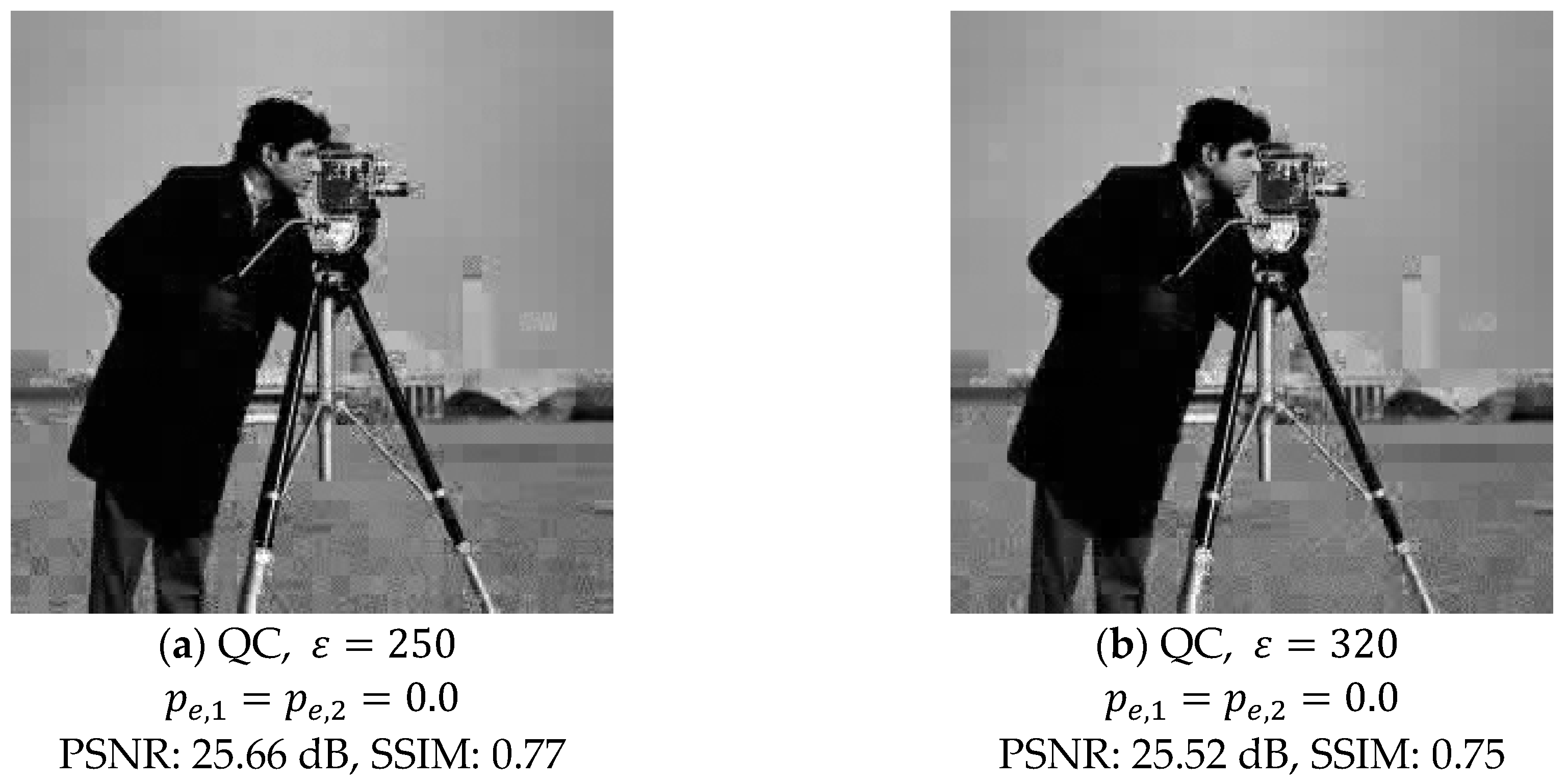
In
Figure 5 we applied adaptive sampling and quadratic constraint with different selections of the value
in Equation (4) for experiments. We chose
for
Figure 5a,c,e, and
for
Figure 5b,d,f. In
Figure 5a,b, we applied error-free transmission, or
, over the two independent and lossy channels. We observed that
Figure 5a, or the one with
, performed slightly better. In
Figure 5c,d, we set
and
, meaning that Channel 1 was lossy, and Channel 2 was error-free. Here we noticed that
Figure 5d, or the one with
, had better PSNR and SSIM values. We also noted that even though the PSNR value in
Figure 5d was larger than that of
Figure 5c, the SSIM value was not. SSIM considers the local characteristics of the images, and PSNR takes the error of the whole image into account. Thus, there may sometimes be mismatches between the two measures. Finally, in
Figure 5e,f, we set
. Due to data loss in both channels, reconstructions in
Figure 5e,f depict inferior results to their counterparts in
Figure 5c,d. Here,
Figure 5f, or the one with
, performed better than
Figure 5e. Based the performances depicted in
Figure 5, we may conclude that with the careful selection of the tolerance value or, in this case,
, a better quality reconstructed image can be acquired.
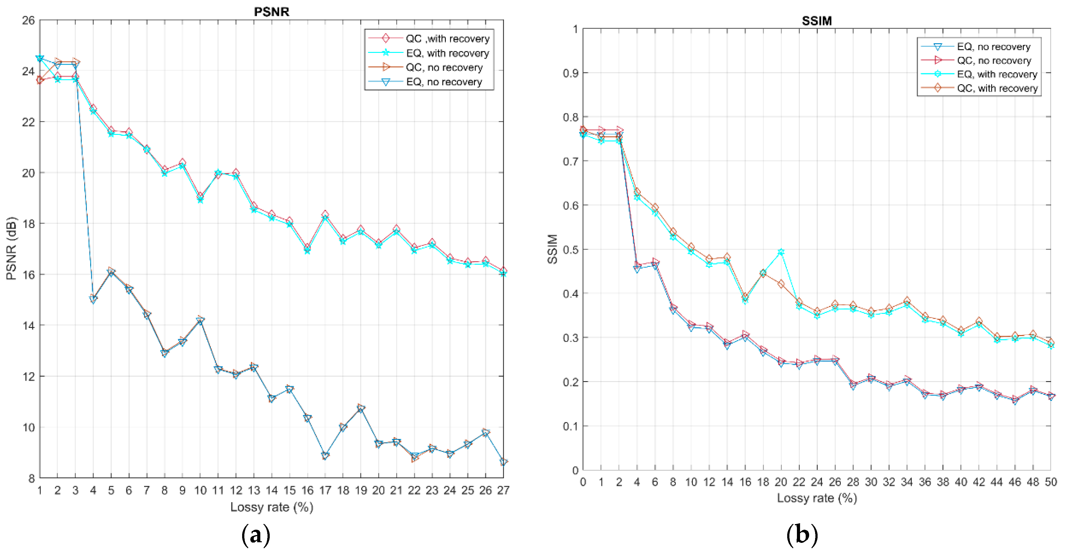
In
Figure 6 we present the evaluations of the reconstructed image quality over a range of lossy probabilities between 0 and 0.5, with a measurement rate of 0.1. We observed that the increase of loss tended toward inferior quality reconstructed images, as was expected. In addition, protection with multiple description coding alleviated the effect caused by data loss, which led to better quality reconstructed images. Finally, we found that with the careful selection of the
value, quadratic constraint performed slightly better than equality constraint in terms of reconstructed image quality.
In
Figure 7,
Figure 8,
Figure 9,
Figure 10 and
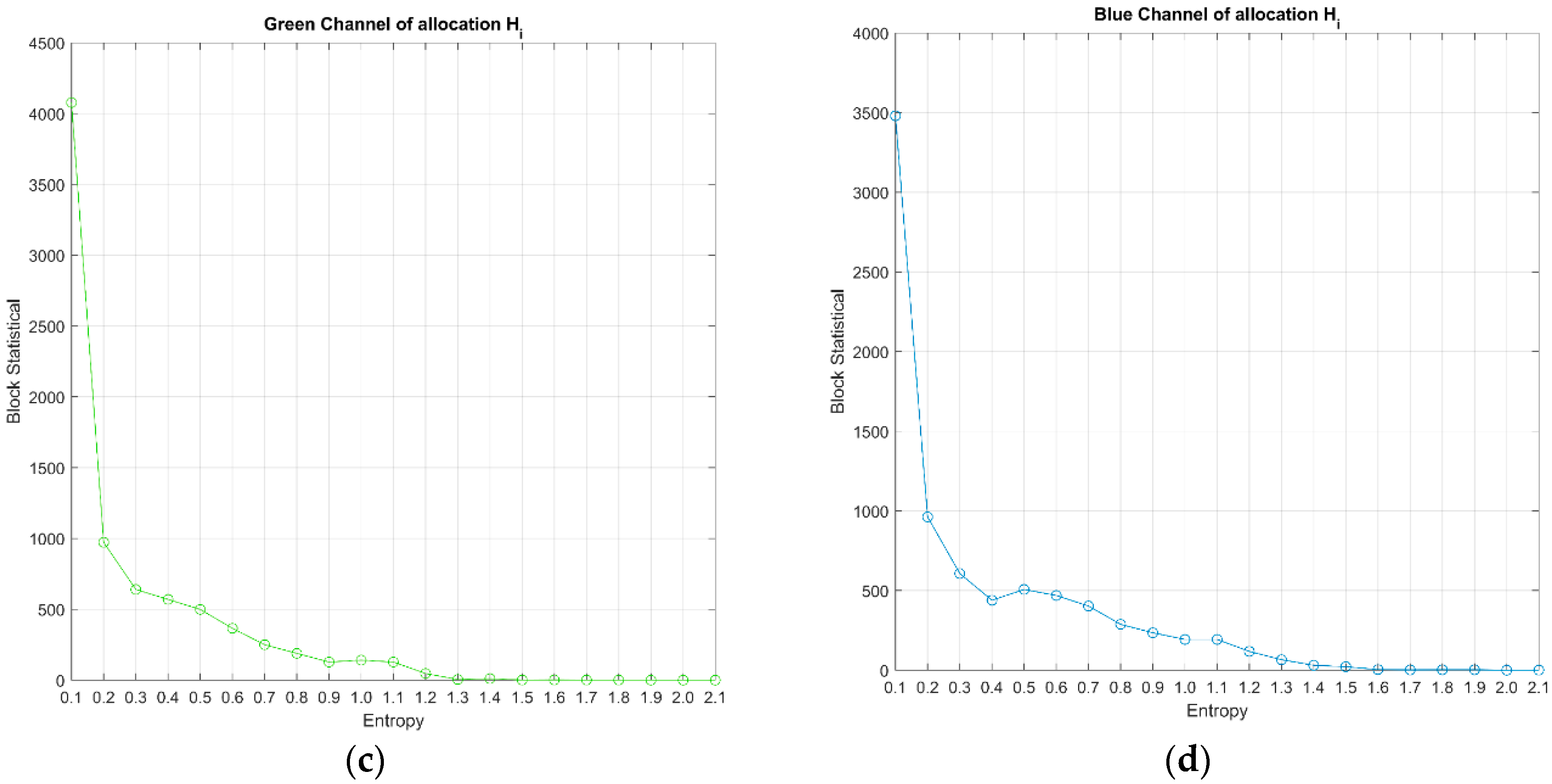
Figure 11 we demonstrate the second set of experiments for the color image ducks with a size of 1024 × 1024. The color image is composed of three color planes, namely, red, green, and blue.
Figure 7a depicts the color image ducks, and
Figure 7b–d shows the entropies in the three color planes for adaptive sampling (AS).
Figure 8 presents the error-free transmission of BCS for ducks. The measurement rate was set to
for each color plane, and reconstructed images can be assessed with the PSNR and SSIM measures. Note that the abbreviations in the captions of
Figure 8 are identical to their counterparts in
Figure 3.
Figure 8a,b show only the reconstruction for equality constraint (EQ) and quadratic constraint (QC), respectively. The PSNR and SSIM values are also shown.
Figure 8c,d present the reconstruction for EQ + AS and QC + AS, respectively.
With adaptive sampling, better PSNR and SSIM performance can be observed. In addition, the performance with QC was slightly better than that with Equation (9). This observation for the color image of ducks in
Figure 8 is similar to that for the grey-level image of cameraman in
Figure 3.
In
Figure 9, we apply the multiple description coding of Equation (9) to protect the BCS coefficients with EQ or QC constraints. Regarding the demonstrations of performance of the proposed method, for the BCS coefficients in the red and green planes we set
, and the BCS coefficients in the blue plane were treated as error-free transmissions or
. In
Figure 9a,c, because the BCS coefficients could be lost during transmission, the degradation of the reconstructed image was affected whether or not the EQ or QC constraints were applied. In
Figure 9b,d, due to high correlation between color planes and protection with multiple description coding, the reconstructed image quality was significantly improved.
In
Figure 10, we provide three sets of angles
and
in MDC with
from Equation (9). First, we chose
and
, which led to opposite signs between angles. Second, we choose
and
, meaning that the two angles were orthogonal. Third, by combining the first two selections, we chose
and
. For
Figure 10a,c,e, reconstruction was based on the equality constraint, while for
Figure 10b,d,f, reconstruction was based on the quadratic constraint. Comparing the three selections, the orthogonal angles may lead to better performance to combat channel errors in reconstruction.
In
Figure 11, we display the evaluations of reconstructed image qualities over the range of lossy probabilities between the range of 0 and 0.5, with a measurement rate of 0.1. We observed that with increased loss rates the inferior quality of the reconstructed images could be monitored. In addition, protection with multiple description coding, or the three curves at the upper portion, alleviated the effect caused by data loss, which led to better quality reconstructed images. Finally, we found that with the careful selection of the
value from Equation (4), quadratic constraint performed slightly better than the equality constraint in reconstructed image quality.
In
Figure 12,
Figure 13,
Figure 14,
Figure 15 and
Figure 16 we demonstrated the results of the third set of experiments for the color image Pasadena-houses with the size of 1760 × 1168. Unlike the test image cameraman in
Figure 3a and ducks in
Figure 7a, which are square-shared images,
Figure 12a was a rectangular-shaped image. The color image was composed of three color planes, namely red, green, and blue.
Figure 12a depicts the color image Pasadena-houses, and
Figure 12b–d displays the entropy distributions of the three color planes for adaptive sampling (AS).
Figure 13 presents the error-free transmission of BCS for Pasadena-houses. The measurement rate was set to
for each color plane whether AS was applied or not. The reconstructed images were assessed with PSNR and SSIM.
Figure 13a,b show the reconstruction for equality constraint (EQ) and quadratic constraint (QC), respectively, and the PSNR and SSIM values are also shown.
Figure 13c,d present the reconstruction for EQ + AS and QC + AS, respectively. With adaptive sampling, better PSNR and SSIM performances were observed due to the local characteristics in entropy distribution. Again, QC performed slightly better than EQ. This observation fit for the color images Pasadena-houses in
Figure 12, ducks in
Figure 8, and the grey-level image cameraman in
Figure 3.
In
Figure 14 we applied multiple description coding from Equation (9) to protect the BCS coefficients with EQ or QC constraints. By following the scenarios in
Figure 9 for the BCS coefficients in the red and green planes, we set
. The BCS coefficients in the blue plane were treated as error-free transmissions, or
. In
Figure 14a,c, because the BCS coefficients could be lost during transmission, the degradation of the reconstructed image was affected whether or not the EQ or QC constraints were applied. In
Figure 14b,d, due to the high correlation between color planes and the protection with multiple description coding, the reconstructed image quality was significantly improved.
In
Figure 15, by following the same parameter settings used in
Figure 10, we provided three sets of selections of angles
and
in MDC with
in Equation (9). First, we chose
and
, which led to opposite signs between angles. Second, we chose
and
, meaning that the two angles were orthogonal. Third, by combining the first two selections, we chose
and
. For
Figure 15a,c,e, reconstruction was based on the equality constraint, while for
Figure 15b,d,f, reconstruction was based on the quadratic constraint. Comparing the three selections, angles that were orthogonal may have led to better performance combatting channel errors in reconstruction.
In
Figure 16 we demonstrated the evaluations of reconstructed image quality over a range of lossy probabilities between 0 and 0.5, with the measurement rate of 0.1. We observed that, with increased loss rates, inferior quality reconstructed images were seen whether or not the protection was deployed. In addition, protection with multiple description coding, or the three curves at the upper portion in
Figure 16a,b, alleviated the effect of data loss, which led to better quality reconstructed images.
From the results of the three sets of experiments, which corresponded to the three test images presented above, cameraman, ducks, and Pasadena-houses, protection of BCS with multiple description coding pointed to the applicability for transmitting over lossy channels. MDC worked together with EQ or QC reconstruction methods for BCS signals. Compensation between received descriptions with MDC helped reduce the effects of lossy channels. The alleviation of reconstructed image quality with error resilient coding is coveted.


