Image Completion with Hybrid Interpolation in Tensor Representation

Abstract

The issue of image completion has been developed considerably over the last two decades, and many computational strategies have been proposed to fill-in missing regions in an incomplete image. When the incomplete image contains many small-sized irregular missing areas, a good alternative seems to be the matrix or tensor decomposition algorithms that yield low-rank approximations. However, this approach uses heuristic rank adaptation techniques, especially for images with many details. To tackle the obstacles of low-rank completion methods, we propose to model the incomplete images with overlapping blocks of Tucker decomposition representations where the factor matrices are determined by a hybrid version of the Gaussian radial basis function and polynomial interpolation. The experiments, carried out for various image completion and resolution up-scaling problems, demonstrate that our approach considerably outperforms the baseline and state-of-the-art low-rank completion methods.

1. Introduction

Image completion aims to synthesize missing regions in an incomplete image or a video sequence with the content-aware information captured from accessible or unperturbed regions. The missing regions may result from removing unwanted sub-areas, occlusion, or unobserved or considerably damaged random pixels.

Image completion is one of the fundamental research topics in the area of computer vision and graphics technology, motivated by widespread applications in various applied sciences [1]. It is used for  the restoration of old photographs, paintings, and films by removing scratches, dust spots, occlusions, or other user-marked objects, such as annotations, subtitles, stamps, logos, etc. In  telecommunications, image completion techniques may fix error concealment problems or recover missing data-blocks lost during transmission or video compression [2,3]. The recent works also emphasize their usefulness in remote sensing imaging to remove occlusions, such as clouds and “dead” pixels [4,5].

The topic of image completion has been extensively studied for at least two decades, resulting in the development of several computational approaches to address this problem. The pioneering work in fully automated digital image inpainting dates back to 2000 when Bertalmio et al. [6] introduced a milestone algorithm that was able to automatically fill in missing regions from their neighboring information without providing user-defined sample images. This algorithm is based on partial differential equations (PDEs) that determine isophotes (brightness-level lines) along which the information on the surrounding structure is propagated upwards. It is a fully automatic algorithm, but it inpaints efficiently only in narrow lines, does not recover textures, and produces blurred results. Another approach to image inpainting is to synthesize the texture. This concept was introduced by Efros and Leung [7] in 1999, but their algorithm requires a sample texture image to recover the texture in the missing region. Bertalmio et al. [8] also developed a hybrid version of both inpainting techniques, in which an incomplete image is decomposed into its texture and structure components, one  reconstructed by texture synthesis, and another by PDE-based image inpainting. When a region to be completed is relatively large, the exemplar-based image synthesis algorithms [9,10,11] or their hybrid versions [12] seem to be more appropriate. The hybrid strategies have been studied in many other research papers [13,14,15,16], and currently, image completion based on simultaneous fill-in of texture and structure is a fundamental approach, especially for recovering large missing regions. Various  neural network architectures, e.g., convolutional neural network and generative adversarial network, can also perform hybrid image completion [17,18,19,20]. A survey of image completion methods can be found in [1,5,21,22].

The above-mentioned image completion methods are efficient even for very large missing regions; however, they cannot be applied for incomplete images with many uniformly distributed missing pixels (e.g., about 90 %). No texture information can be learned from any subregions of such an image. There is also no continuous boundary of missing regions, and hence the neighboring information cannot be propagated towards the centers of missing regions. In such cases, different methods must be applied. Assuming that an incomplete image has a low-rank structure and satisfies the incoherence condition [23], usually represented by clusters of similar patches, the image completion boils down to a rank minimization problem. Since it is an NP-hard problem, many computational strategies have been proposed to approximate it by a convex relaxation, usually involving matrix or tensor decomposition methods. One of them assumes a convex approximation of a rank minimization problem with a nuclear-norm minimization problem, which can be solved easily using singular value decomposition (SVD) [24,25,26]. Due to the orthogonality condition, low-rank representations yielded by SVD contain negative values, which is not profitable for representing a large class of images. Other low-rank models (not necessarily restricted to SVD) can be used to tackle this problem [27].

One of the commonly used methods for extracting low-rank part-based representations from nonnegative matrices is nonnegative matrix factorization (NMF) [28]. It has already found many relevant applications in image analysis, and can also be used for solving image completion problems [29,30]. In this approach, the missing regions are sequentially updated with an NMF-based low-rank approximation of an observed image, which resembles the phenomena of propagating the neighboring information towards the missing regions in the PDE-based inpainting methods. However, due to the non-convexity of alternating optimization, NMF is sensitive to its initialization, especially for insufficiently sparse data. The ambiguity effects can be considerably relaxed if tensor decomposition models are used [31]. Moreover, multi-linear decomposition models prevent cross-modal interactions, which is particularly useful for image representations. Such a low-rank image completion methodology is mostly based on the concept of tensor completion issues that have been extensively studied [32,33,34,35,36]. There are many tensor decomposition models that are used for image completion tasks, including the fundamental ones, such as CANDECOMP/PARAFAC (CP) [37,38] and Tucker decomposition [39,40,41], as well as tensor networks, such as tensor ring [42], tensor train [43,44], hierarchical Tucker decomposition [45], and other tensor decomposition models [46].

Tensor completion methods are intrinsically addressed for processing color images (3D multi-way arrays), but they can also be applied to gray-scale images using various tensorization or scanning operators, e.g., the ket augmentation [47]. They are also very flexible in incorporating penalty terms or constraints; however, their efficiency strongly depends on the image to be completed. In practice, a low-rank representation is always a certain approximation of the underlying image, controlled by the rank of a tensor decomposition model. The problem of rank selection is regarded in terms of a trade-off between under- and over-fitting, and many approaches exist to tackle it. For example, Yokota et al. [38] proposed to increase the rank with recursive updates. In the early recursive steps, a low-rank structure is recovered, and then it is gradually updated to a higher-rank structure that contains more details. The rank can also be controlled by the decreasing rank procedure [46] or using the singular value thresholding strategy [43]. Thus, one of the drawbacks of this kind of image completion method is the problem of selecting the optimal rank of decomposition, and it is usually resolved by heuristic procedures. Moreover, the tensor decomposition-based image-completion methods usually involve a high computational cost if all factor matrices or core tensors are updated in each iterative step.

To relax the problem with the right rank selection while keeping computational costs at a very low level, we propose a very simple alternative approach to low-rank image completion. Our strategy is based on the Tucker decomposition model in which the full-rank factor matrices are previously estimated with a hybrid connection of two interpolation methods. Since the factor matrices are precomputed, only the core tensor must be estimated. Despite the full-rank assumption, it involves a relatively low computational cost because the core tensor is sparse with non-zero entries determined by the available pixels. Motivated by several works [48,49,50,51] on the use of various interpolation methods for solving image completion problems, other recent works [52,53,54,55,56] on image processing aspects, and the concept of tensor product spline surfaces [57], we show the relationship of the Tucker decomposition with factorizable radial basis function (RBF) interpolation and use it to compute the factor matrices. RBF interpolation is a mesh-free method, which is very profitable for recovering irregularly distributed missing pixels, but it may incorrectly approximate linear structure. Hence, we combine it with low-degree polynomial interpolation, and both interpolation methods can be expressed by the Tucker decomposition model. Adopting the idea of PDE-based inpainting, we propose to compute the interpolants using only restricted surrounding subareas, instead of all accessible pixels. Hence, the whole image is divided into overlapping blocks, and the Tucker decomposition model is applied to each block separately. As many interpolation methods do not approximate the boundary entries well, the overlapping is necessary to avoid discontinuity effects. The proposed methodology is applied to various image completion problems, where the incomplete images are obtained from true images by removing many random pixels or many small holes. One of the experiments is performed for resolution up-scaling, where a low-resolution image is up-scaled to high resolution using the proposed algorithm. All the experiments demonstrate that the proposed method considerably outperforms the baseline and state-of-the-art low-rank image-completion methods in terms of the performance, and it is much faster than the methods based on tensor decompositions.

The remainder of this paper is organized as follows. Section 2 reviews some preliminary knowledge about fundamental tensor operations, the Tucker decomposition model, low-rank tensor completion, and RBF interpolation. The proposed algorithm is described in Section 3. The numerical experiments performed on various image completion problems are given and discussed in Section 4. The last section contains the conclusions.

2. Preliminary

Mathematical notations and preliminaries of tensor decomposition models are adopted from [31]. Tensors are multi-way arrays, denoted by calligraphic letters (e.g., $\mathcal{Y}$). Let $\mathcal{Y}\in {\mathbb{R}}^{I_1\times \dots \times I_N}$ be the N-way array. The elements of $\mathcal{Y}$ are denoted as $y_{i_1,\dots ,i_N}$, where $\forall n:1\le i_n\le I_n$, $n=1,\dots ,N$. Boldface uppercase letters (e.g., Y ) denote matrices; lowercase boldface ones stand for vectors (e.g., y); non-bold letters are scalars. The vector $y_j$ contains the j-th column of Y. The symbol $\left|\right|·{\left|\right|}_{\mathit{F}}$ denotes the Frobenius norm of a matrix; $\left|\right|·\left|\right|$ denotes the 2-nd norm. The sets of real numbers and natural numbers are represented by $\mathbb{R}$ and $\mathcal{N}$, respectively. The symbols $\lfloor x\rfloor$ and $\lceil x\rceil$ stand for the floor and ceiling functions of x, respectively.

Let $\mathcal{M}=[m_{i_1,\dots ,i_N}]\in {\mathbb{R}}^{I_1\times \dots \times I_N}$ be the N-th way observed tensor with missing entries, and $\mathsf{\Omega }=[{\omega }_{i_1,\dots ,i_N}]\in {\mathbb{R}}^{I_1\times \dots \times I_N}$ be a binary tensor that indicates the locations of available entries in $\mathcal{M}$. If $m_{i_1,\dots ,i_N}$ is observed, then ${\omega }_{i_1,\dots ,i_N}=1$; otherwise, ${\omega }_{i_1,\dots ,i_N}=0$. The locations of positive entries in $\overline{\mathsf{\Omega }}=1-\mathsf{\Omega }$ correspond to missing entries in $\mathcal{M}$. The number of observed entries is equal to $|\mathsf{\Omega }|=\{♯(i_1,\dots ,i_N):{\omega }_{i_1,\dots ,i_N}>0\}$.

Definition 1.

Let

$$\begin{array}{c}\hfill \widehat{\mathcal{Y}}=[{\widehat{y}}_{i_1,\dots ,i_N}],\mathrm{where}{\widehat{y}}_{i_1,\dots ,i_N}=\left\{\begin{array}{ccc}{m}_{i_1,\dots ,i_N}\hfill & \mathrm{if}& {\omega }_{i_1,\dots ,i_N}=1,\\ 0\hfill & \mathrm{otherwise}\end{array}\right.\end{array}$$

(1)

be a zero-filled incomplete tensor.

Definition 2.

Let

$$\begin{array}{c}\hfill \mathcal{Y}\left(\mathsf{\Omega }\right)=[{\overline{y}}_{i_1,\dots ,i_N}],\mathrm{where}{\overline{y}}_{i_1,\dots ,i_N}=\left\{\begin{array}{ccc}{m}_{i_1,\dots ,i_N}\hfill & \mathrm{if}& {\omega }_{i_1,\dots ,i_N}=1,\\ \varnothing \hfill & \mathrm{otherwise}\end{array}\right.\end{array}$$

(2)

be a subtensor of $\mathcal{M}$ that contains only the entries pointed to by Ω.

Thus: $\left|\mathcal{Y}\right(\mathsf{\Omega }\left)\right|=\left|\mathsf{\Omega }\right|$. Let $\mathit{\omega }=\mathrm{vec}\left(\mathsf{\Omega }\right)\in {\mathbb{R}}^{{\prod }_{n=1}^N{I}_n}$ be a vectorized version of $\mathsf{\Omega }$.

2.1. Image Completion with Tucker Decomposition

For the N-th order tensor $\mathcal{Y}\in {\mathbb{R}}^{I_1\times I_2\times \dots \times I_N}$, the Tucker decomposition [58] with the ranks $J=(J_1,J_2,\dots ,J_N)$ can be formulated as

$$\mathcal{Y}=\mathcal{G}{\times }_1{\mathit{U}}^{\left(1\right)}{\times }_2{\mathit{U}}^{\left(2\right)}{\times }_3\dots {\times }_N{\mathit{U}}^{\left(N\right)},$$

(3)

where $\mathcal{G}=[g_{j_1,\dots ,j_N}]\in {\mathbb{R}}^{J_1\times J_2\times \dots \times J_N}$ for $J_n\le I_n$ is the core tensor, and ${\mathit{U}}^{\left(n\right)}=[{\mathit{u}}_1^{\left(n\right)},\dots ,{\mathit{u}}_{J_n}^{\left(n\right)}]=[u_{i_n,j_n}]\in {\mathbb{R}}^{I_n\times J_n}$ for $n=1,\dots ,N$ is the factor matrix capturing the features across the n-th mode of $\mathcal{Y}$. The operator ${\times }_n$ stands for the standard tensor-matrix contraction along the n-th mode, which is defined as

$$\begin{array}{c}\hfill {\left[\mathcal{G}{\times }_n{\mathit{U}}^{\left(n\right)}\right]}_{j_1,\dots ,j_{n-1},i_n,j_{n+1},\dots ,j_N}=\sum _{j_n=1}^{J_n}{g}_{j_1,\dots ,j_N}{u}_{i_n,j_n}^{\left(n\right)}.\end{array}$$

(4)

The optimization problem for low-rank image completion with the Tucker decomposition can be formulated as follows:

$$\begin{array}{c}\underset{\mathcal{Z},\mathcal{G},{\mathbf{U}}^{\left(1\right)},\dots ,{\mathbf{U}}^{\left(N\right)}}{min}\frac{1}{2}\left|\right|\mathcal{Z}-{\mathcal{Y}\left|\right|}_{\mathit{F}}^2+\mathsf{\Phi }(\mathcal{G},\{{\mathit{U}}^{\left(n\right)}\}),\mathrm{s}.\mathrm{t}.{\mathcal{Z}}_{\mathsf{\Omega }}={\mathcal{M}}_{\mathsf{\Omega }},{\mathcal{Z}}_{\mathsf{\Omega }}\ge 0,\hfill \\ \forall n,j_n:\left|\right|u_{j_n}^{\left(n\right)}\left|\right|=1,j_n=1,\dots ,J_n,n=1,\dots N.\hfill \end{array}$$

(5)

where $\mathcal{Y}$ is given by model (3), and $\mathsf{\Phi }(·)$ is a penalty function that imposes the desired constraints onto the core tensor $\mathcal{G}$ and the factor matrices $\{{\mathit{U}}^{\left(n\right)}\}$. The projection ${\mathcal{Z}}_{\mathsf{\Omega }}={\mathcal{M}}_{\mathsf{\Omega }}$ means that $z_{i_1,\dots ,i_N}$ is  replaced with $m_{i_1,\dots ,i_N}$ if ${\omega }_{i_1,\dots ,i_N}=1$; otherwise, no changes. Assuming $\forall n:J_n<I_n$, the tensor $\mathcal{Y}$ in (3) has a low Tucker rank.

Problem (5) can be solved by performing iterative updates with the Tucker decomposition in each  step. The Tucker decomposition can be computed in many ways, depending on the constraints imposed on the estimated factors. If the nonnegativity constraints are used (as specified), any  nonnegative least square (NNLS) solver can be applied in the alternating optimization scheme. Neglecting the computational cost of using an NNLS solver and the cost of computing the core $\mathcal{G}$ in (3), the total computational complexity for approximating the solution to (5) in K iterations can be roughly estimated as $\mathcal{O}(K{\sum }_{n=1}^N{J}_n{\prod }_{p=1}^N{I}_p)$.

2.2. RBF Interpolation

The RBF interpolation [59] is a commonly used mesh-free method for approximating unstructured and high-dimensional data with high-order interpolants. Given the set of I distinct data points $(x_i,y_i)$ for $i=1,\dots ,I$, $\forall i:{\mathit{x}}_i\in {\mathbb{R}}^{\mathit{P}},y_i\in \mathbb{R}$, the aim is to find the approximating function $y\left(x\right)$, which is referred to as the interpolant, satisfying the condition: $\forall i:y\left(x_i\right)=y_i$. For the RBFs $\psi :[0,\infty )\to \mathbb{R}$, the interpolant takes the form

$$\begin{array}{c}\hfill y\left(\mathit{x}\right)=\sum _{j=1}^J{w}_j\psi \left(\left|\right|\mathit{x}-{\mathit{x}}_j\left|\right|\right),\end{array}$$

(6)

where $\left\{w_i\right\}$ are real-value weighting coefficients. For I data points, we have

$$\begin{array}{c}\hfill y_i=\sum _{j=1}^J{w}_j\psi \left(\left|\right|{\mathit{x}}_i-{\mathit{x}}_j\left|\right|\right),\mathrm{where}i=1,\dots ,I\end{array}$$

(7)

The weighting coefficients $\left\{w_i\right\}$ can be computed from the system of linear equations:

$$\begin{array}{c}\hfill \mathit{y}=\mathbf{\Psi }\mathit{w},\end{array}$$

(8)

where $\mathit{y}={[y_1,\dots ,y_I]}^T\in {\mathbb{R}}^I$, $\mathbf{\Psi }=\left[\psi \left(\left|\right|x_i-x_j\left|\right|\right)\right]\in {\mathbb{R}}^{I\times J}$, and $w={[w_1,\dots ,w_J]}^T\in {\mathbb{R}}^J$. If $I\ge J$ and $\mathbf{\Psi }$ is a full-rank matrix, system (8) can be solved with any linear least-square solver.

3. Proposed Algorithm

For interpolation of N-way incomplete tensor $\mathcal{M}$, the points ${\mathit{x}}_i$ and ${\mathit{x}}_j$ in (7) are expressed by index values: ${\mathit{x}}_i=[i_1,i_2,\dots ,i_N]\in {\mathbb{R}}^N$ and ${\mathit{x}}_j=[j_1,j_2,\dots ,j_N]\in {\mathbb{R}}^N$. The distance measure in (6) can also be regarded in a wider sense, and hence the norm $l_2$ can be replaced with the distance function $D({\mathit{x}}_i,{\mathit{x}}_j)$. For any distance function, the following conditions are satisfied: $D(\mathit{x},\mathit{x})=0$, $\forall \mathit{x}\ne \mathit{y}:D(\mathit{x},\mathit{y})>0$, $D(\mathit{x},\mathit{y})=D(\mathit{y},\mathit{x})$, and $D(\mathit{x},\mathit{z})\le D(\mathit{x},\mathit{y})+D(\mathit{y},\mathit{z})$. In the N-dimensional space, any data point $y_{i_1,\dots ,i_N}$ can be modelled with the interpolant

$$\begin{array}{ccc}{y}_{i_1,i_2,\dots ,i_N}\hfill & =\hfill & \sum _{j=1}^J{w}_j\psi \left(-\frac{D(x_i,x_j)}{\tau }\right)\hfill \\ \hfill & =\hfill & \sum _{j_1=1}^{J_1}\sum _{j_2=1}^{J_2}\cdots \sum _{j_N=1}^{J_N}{w}_{j_1,j_2,\dots ,j_N}\psi \left(-\frac{D([i_1,i_2,\dots ,i_N],[j_1,j_2,\dots ,j_N])}{\tau }\right),\hfill \end{array}$$

(9)

where $\tau >0$ is a scaling factor.

Let $D([i_1,i_2,\dots ,i_N],[j_1,j_2,\dots ,j_N])$ be an additively separable distance function, i.e.,

$$\begin{array}{c}\hfill D([i_1,i_2,\dots ,i_N],[j_1,j_2,\dots ,j_N])=\sum _{n=1}^N{d}^{\left(n\right)}(i_n,j_n),\end{array}$$

(10)

where $d^{\left(n\right)}(i_n,j_n)$ is a one-variable function that expresses the distance metrics for the variables $(i_n,j_n)$ in the n-th mode. We also assume that the RBF $\psi$ is multiplicatively separable. That is

$$\begin{array}{c}\hfill \psi \left(\sum _{n=1}^N{x}_n\right)=\prod _{n=1}^N{\psi }^{\left(n\right)}\left(x_n\right).\end{array}$$

(11)

Considering separability conditions (10), (11), model (9) can be reformulated as follows:

$$\begin{array}{cc}{y}_{i_1,\dots ,i_N}\hfill & =\sum _{j_1=1}^{J_1}\cdots \sum _{j_N=1}^{J_N}{w}_{j_1,\dots ,j_N}\psi \left(-\frac{{\sum }_{n=1}^N{d}^{\left(n\right)}(i_n,j_n)}{\tau }\right)\hfill \\ & =\sum _{j_1=1}^{J_1}\cdots \sum _{j_N=1}^{J_N}{w}_{j_1,\dots ,j_N}\prod _{n=1}^N{\psi }^{\left(n\right)}\left(-\frac{d^{\left(n\right)}(i_n,j_n)}{\tau }\right)=\sum _{j_1=1}^{J_1}\cdots \sum _{j_N=1}^{J_N}{w}_{j_1,\dots ,j_N}\prod _{n=1}^N{f}_{i_n,j_n}^{\left(n\right)}\hfill \\ & =\sum _{j_N=1}^{J_N}\cdots \left(\sum _{j_1=1}^{J_1}{w}_{j_1,\dots ,j_N}{f}_{i_1,j_1}^{\left(1\right)}\right)f_{i_N,j_N}^{\left(N\right)},\hfill \end{array}$$

(12)

where $f_{i_n,j_n}^{\left(n\right)}={\psi }^{\left(n\right)}\left(-\frac{d^{\left(n\right)}(i_n,j_n)}{\tau }\right)$.

Following the standard tensor-matrix contraction rule given in (4), formula (12) can be presented in the following form:

$$\begin{array}{c}\hfill \mathcal{Y}=\mathcal{W}{\times }_1{\mathit{F}}^{\left(1\right)}{\times }_2\dots {\times }_N{\mathit{F}}^{\left(N\right)},\end{array}$$

(13)

where $\mathcal{Y}=[y_{i_1,\dots ,i_N}]\in {\mathbb{R}}^{I_1\times \dots \times I_N}$, $\mathcal{W}=[w_{j_1,\dots ,j_N}]\in {\mathbb{R}}^{J_1\times \dots \times J_N}$, and $\forall n:{\mathit{F}}^{\left(n\right)}=[f_{i_n,j_n}^{\left(n\right)}]\in {\mathbb{R}}^{I_n\times J_n}$.

Remark 1.

The model given in (13) has a form identical to model (3), where$\mathcal{W}$is the core tensor, and$\{{\mathit{F}}^{\left(n\right)}\}$are factor matrices. Hence, the RBF interpolation model in N-dimensional space, in which separability conditions (10), (11) are satisfied, boils down to the Tucker decomposition model, where the factor matrices$\{{\mathit{F}}^{\left(n\right)}\}$are previously determined by rational functions.

If $d^{\left(n\right)}(i_n,j_n)=i_n^{j_n-1}$ is expressed by an exponential function, $\tau =1$, and  $\psi \left(\xi \right)=-\xi$, then $f_{i_n,j_n}^{\left(n\right)}={\psi }^{\left(n\right)}\left(-\frac{d^{\left(n\right)}(i_n,j_n)}{\tau }\right)=i_n^{j_n-1}$, and model (12) takes the form of the standard multivariate polynomial regression:

$$\begin{array}{c}\hfill y_{i_1,\dots ,i_N}=\sum _{j_1=1}^{J_1}\cdots \sum _{j_N=1}^{J_N}{w}_{j_1,\dots ,j_N}\prod _{n=1}^N{\left(i_n\right)}^{j_n-1},\end{array}$$

(14)

where numbers $(J_1,\dots ,J_N)$ determine the degrees of the polynomial with respect to each mode, i.e.,$\forall n:J_n=D_n+1$, where $D_n$ is a degree of the polynomial along the n-th mode. Thus the multivariate polynomial regression can be also presented in the form of the Tucker decomposition model.

The RBF $\psi$ can take various forms, such as Gaussian, polyharmonic splines, multiquadrics, inverse  multiquadrics, and inverse quadratics [59]. The Gaussian RBF (GRBF), expressed by $\psi \left(\xi \right)=exp\left\{\xi \right\}$, is commonly used for interpolation; however, it cannot be used for constructing an interpolant with polynomial precision. For example, the GRBF does not approximate a linear function $y\left(x\right)$ well. Hence, the polynomial regression in (14) is more suitable for linear or slowly varying functions, but it often yields underestimated interpolants if the polynomial has too low of a degree. An increase in the degree leads to an ill-conditioned regression problem and unbiased least squares estimates. To tackle this problem, both interpolation approaches can be combined, which leads to the following interpolation model:

$$\begin{array}{ccc}\hfill y_{i_1,\dots ,i_N}& =& \sum _{j_1=1}^{J_1}\cdots \sum _{j_N=1}^{J_N}{w}_{j_1,\dots ,j_N}\prod _{n=1}^{N}exp\left(-\frac{d^{\left(n\right)}(i_n,j_n)}{\tau }\right)+\sum _{r_1=1}^{R_1}\cdots \sum _{r_N=1}^{R_N}{c}_{r_1,\dots ,r_N}\prod _{n=1}^N{\left(i_n\right)}^{r_n-1}.\hfill \end{array}$$

(15)

Model (15) can be equivalently presented in the tensor-matrix contraction form:

$$\begin{array}{c}\hfill \mathcal{Y}=\mathcal{W}{\times }_1{\mathit{F}}^{\left(1\right)}{\times }_2\dots {\times }_N{\mathit{F}}^{\left(N\right)}+\mathcal{C}{\times }_1{\mathit{P}}^{\left(1\right)}{\times }_2\dots {\times }_N{\mathit{P}}^{\left(N\right)},\end{array}$$

(16)

where $\mathcal{C}=[c_{r_1,\dots ,r_N}]\in {\mathbb{R}}^{R_1\times \dots \times R_N}$ is the core tensor of the polynomial regression model, and $\forall n:{\mathit{P}}^{\left(n\right)}=[p_{i_n,r_n}^{\left(n\right)}]=[1,i_n,i_n^2,\dots ,i_n^{R_n-1}]\in {\mathbb{R}}^{I_n\times R_n}$ is the respective factor matrix with $p_{i_n,r_n}^{\left(n\right)}=i_n^{r_n-1}$. System (16) has ${\prod }_{n=1}^N{J}_n+{\prod }_{n=1}^N{R}_n$ variables, and only ${\prod }_{n=1}^N{I}_n$ equations, resulting in ambiguity of its solution under the assumption that $\forall n:J_n=I_n$. To relax this problem, a side-condition is imposed:

$$\begin{array}{c}\hfill \mathcal{W}{\times }_1{\mathit{P}}^{\left(1\right)T}{\times }_2\dots {\times }_N{\mathit{P}}^{\left(N\right)T}=0.\end{array}$$

(17)

Vectorizing models (16), (17) and performing the straightforward mathematical operations, we get

$$\begin{array}{c}\hfill \left[\begin{array}{c}\mathit{y}\\ 0\end{array}\right]=\left[\begin{array}{cc}\mathit{F}& \mathit{P}\\ {\mathit{P}}^T& 0\end{array}\right]\left[\begin{array}{c}\mathit{w}\\ \mathit{c}\end{array}\right],\end{array}$$

(18)

where $\mathit{y}=\mathrm{vec}\left(\mathcal{Y}\right)\in {\mathbb{R}}^{{\prod }_{n=1}^N{I}_n}$, $\mathit{F}={\mathit{F}}^{\left(N\right)}\otimes \dots \otimes {\mathit{F}}^{\left(1\right)}\in {\mathbb{R}}^{{\prod }_{n=1}^N{I}_n\times {\prod }_{n=1}^N{J}_n}$, $\mathit{P}={\mathit{P}}^{\left(N\right)}\otimes \dots \otimes {\mathit{P}}^{\left(1\right)}\in {\mathbb{R}}^{{\prod }_{n=1}^N{I}_n\times {\prod }_{n=1}^N{R}_n}$, $\mathit{w}=\mathrm{vec}\left(\mathcal{W}\right)\in {\mathbb{R}}^{{\prod }_{n=1}^N{J}_n}$, and $\mathit{c}=\mathrm{vec}\left(\mathcal{C}\right)\in {\mathbb{R}}^{{\prod }_{n=1}^N{R}_n}$. The symbol ⊗ denotes the Kronecker product, and $\mathrm{vec}(·)$ means the vectorization operator.

To apply model (16) for image completion, let $\widehat{\mathcal{Y}}$ be obtained according to Definition 1. System (18) can be applied to model non-zero entries in $\widehat{\mathcal{Y}}$, using the following transformations: $\widehat{y}=\mathrm{vec}\left(\widehat{\mathcal{Y}}\right)=S\mathrm{vec}\left(\mathcal{Y}\right)$, $\widehat{\mathit{F}}=\mathit{S}\mathit{F}\mathit{S}$, $\widehat{\mathit{P}}=\mathit{S}\mathit{P}$, and $\widehat{\mathit{w}}=\mathit{S}\mathit{w}$, where $\mathit{S}=\mathrm{diag}\left\{\mathrm{vec}\left(\mathsf{\Omega }\right)\right\}\in {\mathbb{R}}^{{\prod }_{p=1}^N{I}_p\times {\prod }_{p=1}^N{I}_p}$ is a diagonal matrix with binary values on the main diagonal. The matrices $\widehat{\mathit{F}}$ and $\widehat{\mathit{P}}$ have $|\overline{\mathsf{\Omega }}|$ zero-value rows, and $\widehat{\mathit{F}}$ also has the same number of zero-value columns. After removing the zero-value rows and columns from the transformed system, the observed entries in $\mathcal{M}$ can be expressed by the model

$$\begin{array}{c}\hfill \left[\begin{array}{c}\mathit{y}\left(\mathit{\omega }\right)\\ 0\end{array}\right]=\left[\begin{array}{cc}\mathit{F}(\mathit{\omega },\mathit{\omega })& \mathit{P}(\mathit{\omega },:)\\ \mathit{P}{(\mathit{\omega },:)}^T& 0\end{array}\right]\left[\begin{array}{c}\mathit{w}\left(\mathit{\omega }\right)\\ \mathit{c}\end{array}\right],\end{array}$$

(19)

where $\mathit{y}\left(\mathit{\omega }\right)=\mathrm{vec}\left(\mathcal{Y}\left(\mathsf{\Omega }\right)\right)\in {\mathbb{R}}^{\left|\mathsf{\Omega }\right|}$ is a vectorized version of observed entries in $\mathcal{M}$, $\mathit{F}(\mathit{\omega },\mathit{\omega })\in {\mathbb{R}}^{\left|\mathsf{\Omega }\right|\times \left|\mathsf{\Omega }\right|}$ is a submatrix of $\widehat{\mathit{F}}$ by selecting non-zero rows and columns, $\mathit{P}(\mathit{\omega },:)\in {\mathbb{R}}^{\left|\mathsf{\Omega }\right|\times {\prod }_{n=1}^N{R}_n}$ is obtained from $\widehat{\mathit{P}}$ by removing all zero-value rows, and $\mathit{w}\left(\mathit{\omega }\right)=\mathrm{vec}\left(\mathcal{W}\left(\mathsf{\Omega }\right)\right)\in {\mathbb{R}}^{\left|\mathsf{\Omega }\right|}$, taking into account rule (2). Note that $\left|\mathsf{\Omega }\right|<<{\prod }_{n=1}^N{I}_n$, if the number of missing entries in $\mathcal{M}$ is relatively large.

The matrix $\mathit{F}(\mathit{\omega },\mathit{\omega })$ is positive-definite because it is generated by a GRBF. The matrix $\mathit{P}(\mathit{\omega },:)$ might be ill-conditioned if the polynomial functions of higher degrees are used, but the second term in (16) is used to better approximate linear relationships, and hence there is no need to use higher degrees. In this approach, $\forall n:R_n=3$, which leads to second-degree polynomials. The system matrix in (19) is therefore symmetric and positive-definite, and any least-square (LS) solver can be used to compute the vectors $\mathit{w}\left(\mathit{\omega }\right)$ and c from (19), given $\mathit{y}\left(\mathit{\omega }\right)$.

System (18) can also be used to compute the missing entries in $\mathcal{M}$. Having the estimates for $\mathit{w}\left(\mathit{\omega }\right)$ and c, the missing entries can be obtained by solving the following system of linear equations:

$$\begin{array}{c}\hfill \left[\begin{array}{c}\overline{\mathit{y}}\\ 0\end{array}\right]=\left[\begin{array}{cc}\mathit{F}(\overline{\mathit{\omega }},\mathit{\omega })& \mathit{P}(\overline{\mathit{\omega }},:)\\ \mathit{P}{(\mathit{\omega },:)}^T& 0\end{array}\right]\left[\begin{array}{c}\mathit{w}\left(\mathit{\omega }\right)\\ \mathit{c}\end{array}\right],\end{array}$$

(20)

where $\mathit{F}(\overline{\mathit{\omega }},\mathit{\omega })\in {\mathbb{R}}^{|\overline{\mathsf{\Omega }}|\times |\mathsf{\Omega }|}$ is obtained from F by removing the rows and selecting the columns that are indexed by $\mathsf{\Omega }$, and the vector $\overline{\mathit{y}}=\mathit{y}\left(\overline{\mathit{\omega }}\right)$ contains the estimates for the missing entries in $\mathcal{M}$. Hence,  the completed image is expressed by

$$\begin{array}{c}\hfill \mathcal{Y}=[{\mathit{y}}_{i_1,\dots ,i_N}],\mathrm{where}{\mathit{y}}_{i_1,\dots ,i_N}=\left\{\begin{array}{ccc}{m}_{i_1,\dots ,i_N}\hfill & \mathrm{if}& {\omega }_{i_1,\dots ,i_N}=1,\\ {\overline{\mathit{y}}}_{i_1,\dots ,i_N}\hfill & \mathrm{otherwise}\end{array}\right.\end{array}$$

(21)

The system matrix in (19) has the order of $\left|\mathsf{\Omega }\right|+{\prod }_{n=1}^N{R}_n$. Applying Gaussian elimination to (19), the computational complexity amounts to $\mathcal{O}\left(\left(\right|\mathsf{\Omega }|+{\prod }_{n=1}^N{R}_n{)}^3\right)$, and it is relatively large if the number of missing entries in $\mathcal{M}$ is small. It is therefore necessary to reduce the computational complexity for the LS problem associated with (19). To tackle this issue, let input tensor $\widehat{\mathcal{Y}}=\left[{\widehat{\mathcal{Y}}}^{(s_1,\dots ,s_N)}\right]\in {\mathbb{R}}^{I_1\times \dots \times I_N}$ be partitioned into small overlapping subtensors $\{{\widehat{\mathcal{Y}}}^{(s_1,\dots ,s_N)}\}$, where $\forall n:s_n=1,\dots ,S_n$ and $S_n$ is the number of partitions of $\widehat{\mathcal{Y}}$ along its n-th mode. The total number of subtensors is equal to $S_Y={\prod }_{n=1}^N{S}_n$. Each subtensor can be expressed by ${\widehat{\mathcal{Y}}}^{(s_1,\dots ,s_N)}=\left[{\mathit{y}}_{\mathsf{\Gamma }\left(s_1\right),\dots ,\mathsf{\Gamma }\left(s_N\right)}\right]\in {\mathbb{R}}^{L_1\times \dots \times L_N}$, where $\forall n:L_n=\lceil \frac{I_n}{S_n}\rceil \le I_n$. The set $\mathsf{\Gamma }\left(s_n\right)$ contains the indices of the entries in $\widehat{\mathcal{Y}}$ which belong to ${\widehat{\mathcal{Y}}}^{(s_1,\dots ,s_N)}$ along its n-th mode, and it can be expressed by

$$\begin{array}{c}\hfill \forall n:\mathsf{\Gamma }\left(s_n\right)=\left\{\begin{array}{ccc}\left\{\gamma \left(s_n\right)+1,\dots ,\gamma \left(s_n\right)+L_n\right\}\in {\mathcal{N}}^{L_n}\hfill & \mathrm{for}& s_n<S_n\\ \left\{\gamma \left(S_n\right),\dots ,I_n\right\}\hfill & \mathrm{for}& s_n=S_n\end{array}\right.\end{array}$$

(22)

where $\gamma \left(s_n\right)=\lfloor (s_n-1)(L_n-{\eta }_n)\rfloor$. The parameter ${\eta }_n=\lfloor \frac{{\theta }_n{L}_n}{100}\rfloor$ determines the number of overlapping pixels along the n-th mode, and ${\theta }_n\in [0,99]$ expresses the percentage of the overlap along the n-th mode.

The proposed methodology for image completion should be applied separately to each subtensor. The missing pixels are completed using a very limited volume of the input tensor but mostly restricted to their nearest neighborhood. It is thus a strategy that resembles PDE-based image inpainting, but it is much more flexible for highly dissipated known pixels and allows us to reduce the computational cost dramatically. Moreover, the factor matrices $\{{\mathit{F}}^{\left(n\right)}\}$ and $\{{\mathit{P}}^{\left(n\right)}\}$ in (16) are expressed by radial functions, and hence can be precomputed before using the subtensor partitioning procedure. In RBF-based interpolation methods, the samples or pixels that are close to the boundary of the region of interest are usually not well approximated. However, due to overlapping, boundary perturbation effects in our approach are considerably relaxed.

The pseudo-code of the proposed image completion algorithm is presented in Algorithm 1.   

Algorithm 1: Tensorial Interpolation for Image Completion (TI-IC)

Remark 2.

The computational complexity for calculating matrices F and P in Algorithm 1 amounts to$\mathcal{O}\left({\prod }_{n=1}^N{I}_n(J_n+R_n)\right)$. Assuming Gaussian elimination is used for solving system (19), we have$\mathcal{O}\left(S_Y\left(\right|{\mathsf{\Omega }}^{(s_1,\dots ,s_N)}{|+{\prod }_{n=1}^N{R}_n)}^3\right)$for$S_Y$subtensors, and$\mathcal{O}(S_Y(|{\overline{\mathsf{\Omega }}}^{(s_1,\dots ,s_N)}|$+${\prod }_{n=1}^N{R}_n\left)\right(|{\mathsf{\Omega }}^{(s_1,\dots ,s_N)}|+{\prod }_{n=1}^N{R}_n\left)\right)$for computing${\overline{y}}^{(s_1,\dots ,s_N)}$from (20). Let$\left|\mathsf{\Omega }\right|=\xi {\prod }_{n=1}^N{I}_n$and$\forall (s_1,\dots ,s_N):|{\mathsf{\Omega }}^{(s_1,\dots ,s_N)}|=\xi {\prod }_{n=1}^N{L}_n$, where$0\le \xi \le 1$. Neglecting matrix P in (19) because it is much smaller than F, the computational complexity for solving system (19) can be roughly estimated as$\mathcal{O}\left(S_Y\left(\right|{\mathsf{\Omega }}^{(s_1,\dots ,s_N)}{\left|\right)}^3\right)=\mathcal{O}\left(S_Y{\xi }^3{\left({\prod }_{n=1}^N{L}_n\right)}^3\right)\approx \mathcal{O}\left({\xi }^3{\prod }_{n=1}^N\frac{I_n^3}{S_n^2}\right)$. Note that the computational complexity for solving the same system without partitioning tensors$\mathcal{Y}$into subtensors and under the same assumption can be roughly estimated as$\mathcal{O}\left({\left|\mathsf{\Omega }\right|}^3\right)=\mathcal{O}\left({\xi }^3{\prod }_{n=1}^N{I}_n^3\right)$. Hence, the partitioning strategy decreases the computational complexity$S_Y^2$times with respect to the non-partitioned system, and if$\forall n:J_n=I_n$, the complexity for precomputing matrix F might predominate.

4. Results

This section presents an experimental study that was carried out to demonstrate the performance of the proposed algorithms. The tests were performed for a few image completion problems using the following RGB images: Barbara, Lena, Peppers, and Monarch, which are presented in Figure 1. All of them have a resolution of $512\times 512$ pixels.

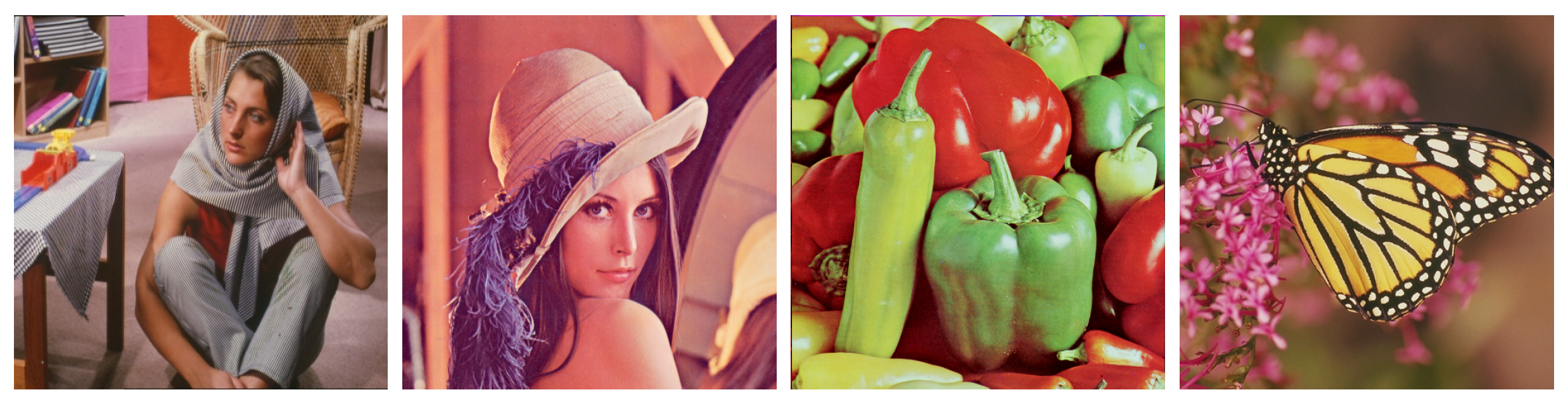
4.1. Setup

The incomplete images were obtained by removing some entries from tensors representing the original images. The following test cases were analyzed:

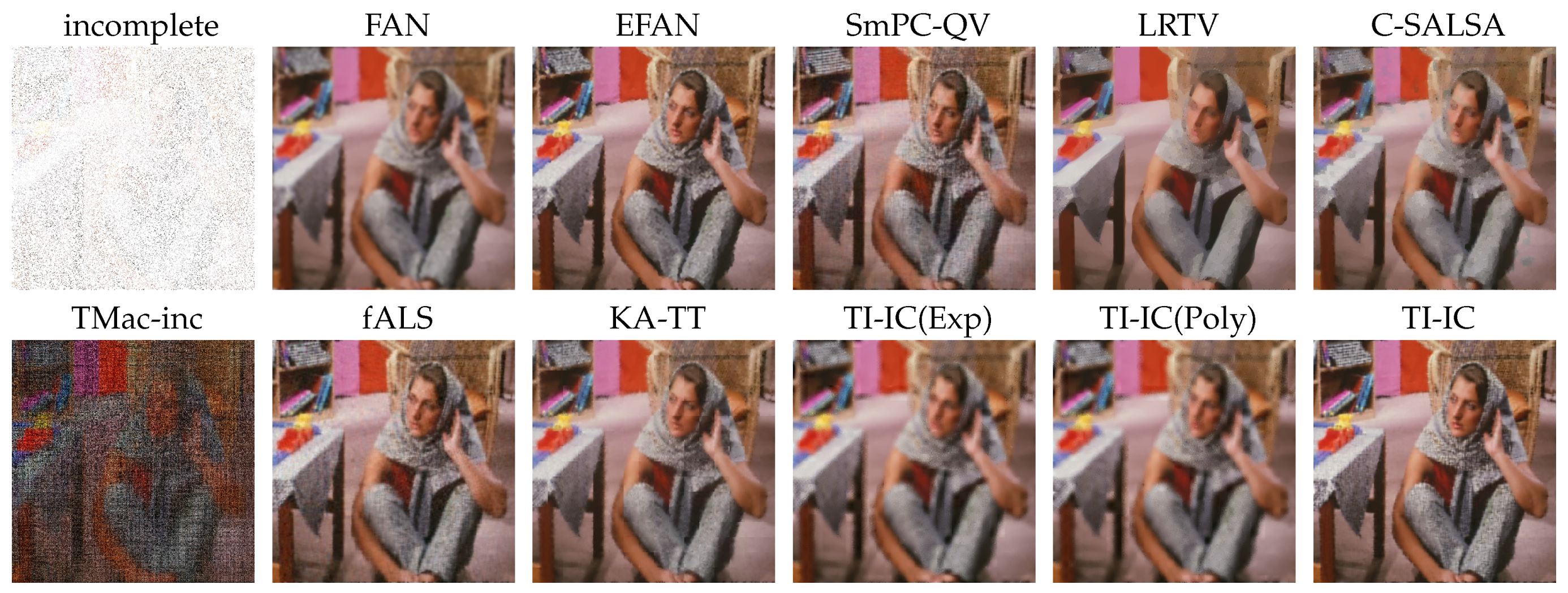
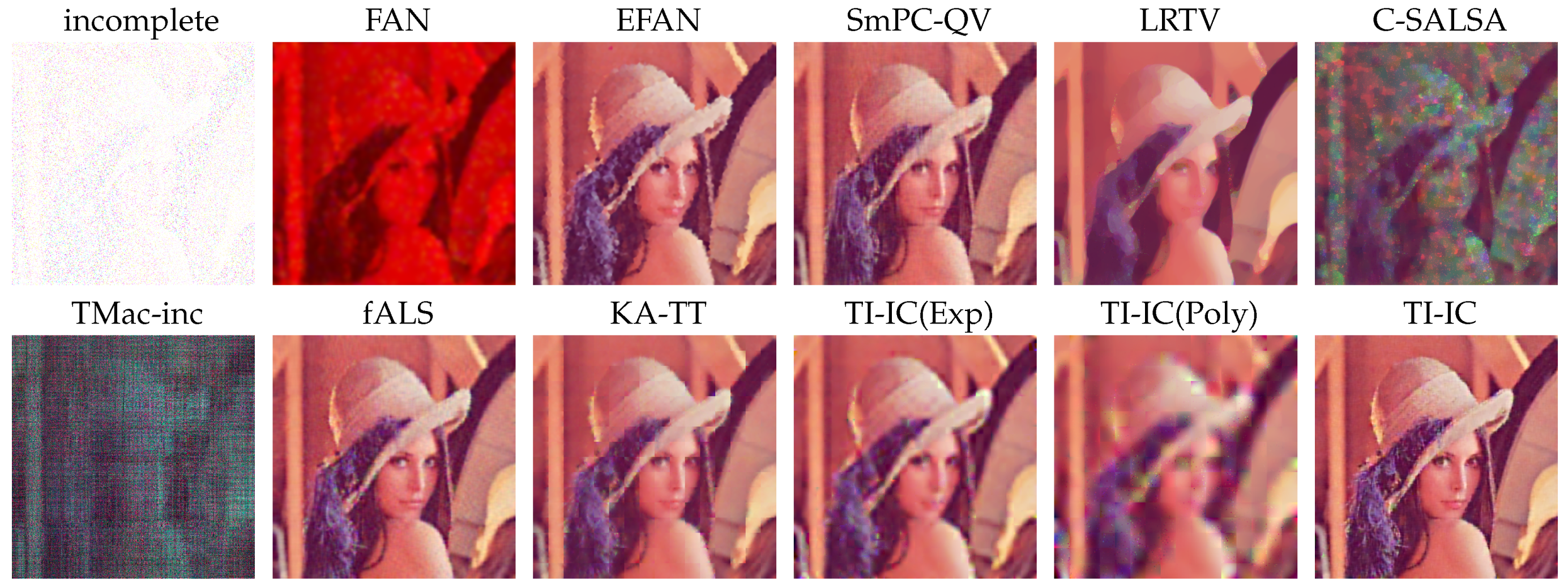
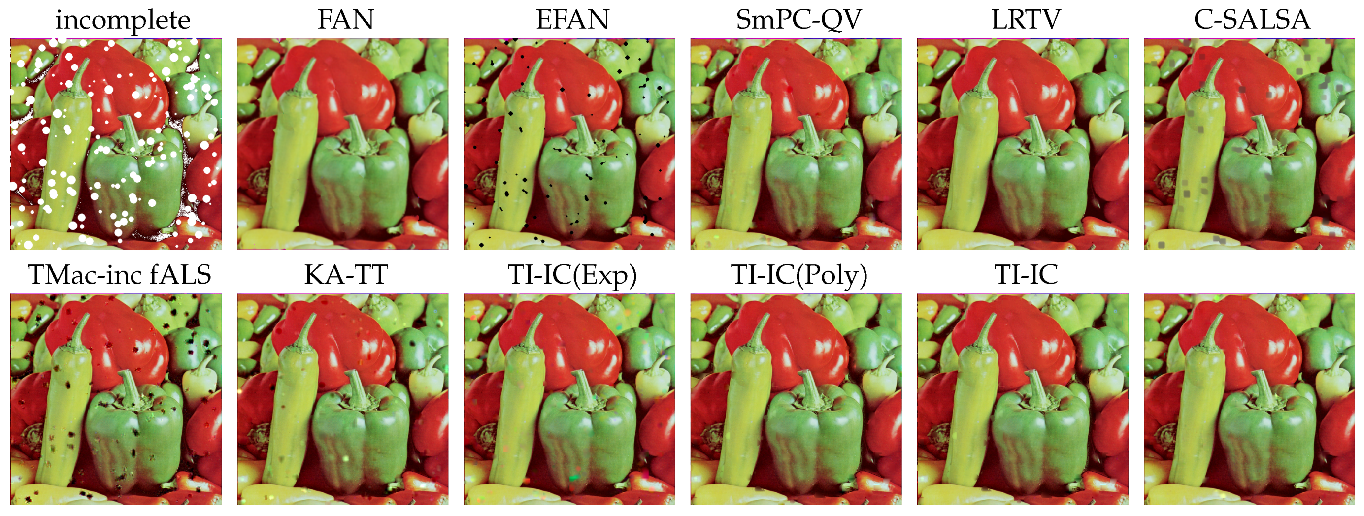
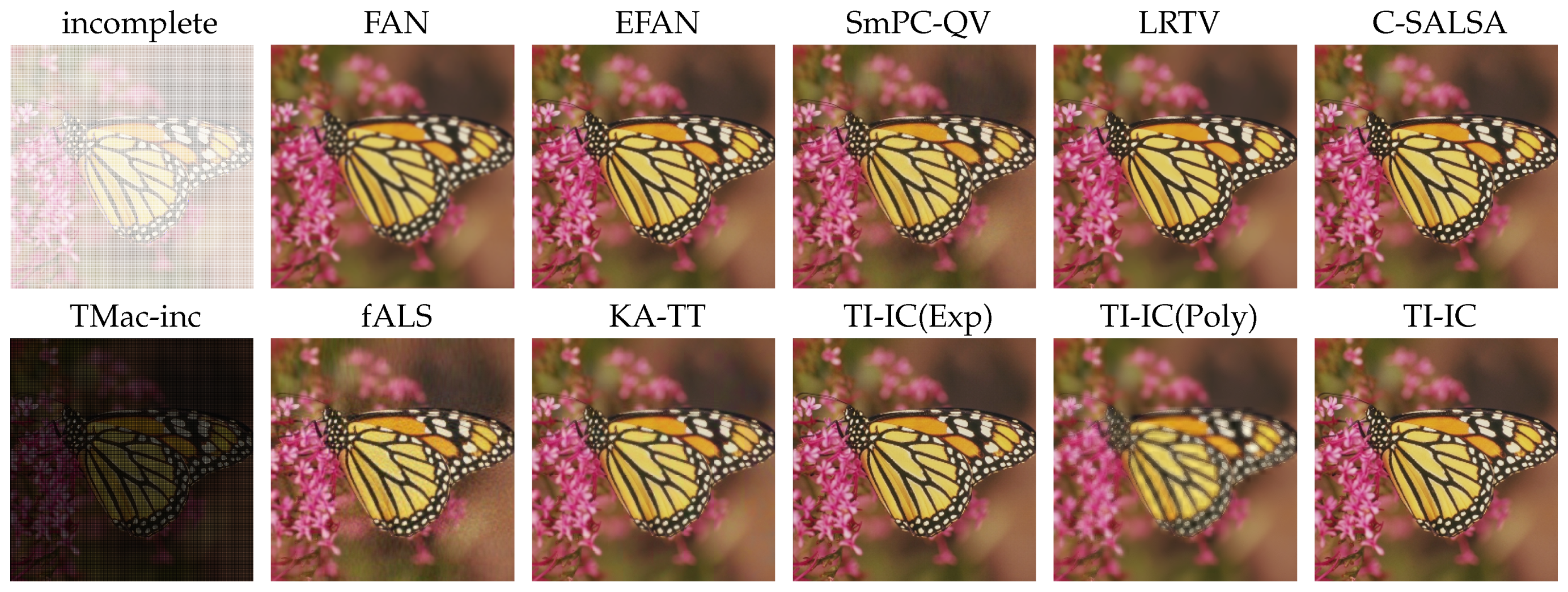
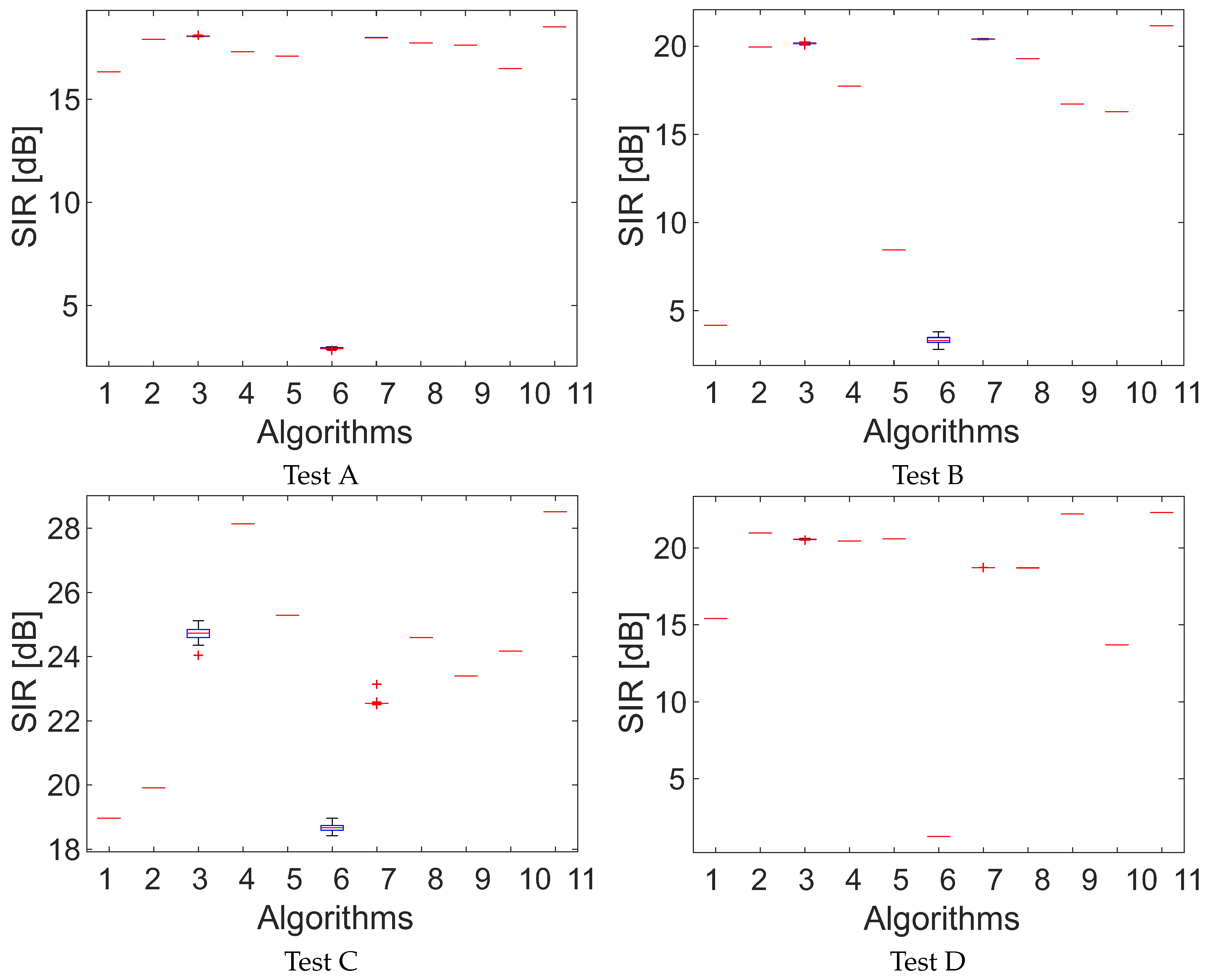
• A: 90% uniformly distributed random missing tensor fibers in its third mode (color), which corresponds to 90% missing pixels (“dead pixels”),
• B: 95% uniformly distributed random missing tensor entries (“disturbed pixels”),
• C: 200 uniformly distributed random missing circles—created in the same way as in the first case, but the disturbances are circles with a random radius not exceeding 10 pixels,
• D: resolution up-scaling—an original image was down-sampled twice by removing the pixels according to a regular grid mask with edges equal to 1 pixel. The aim was to recover the missing pixels on the edges.

We compared the proposed methods with the following: FAN (filtering by adaptive normalization) and EFAN (efficient filtering by adaptive normalization) [60], SmPC-QV (smooth PARAFAC tensor completion with quadratic variation) [38], LRTV (low-rank total-variation) [61], TMAC-inc (low-rank tensor completion by parallel matrix factorization with the rank-increasing) [62], C-SALSA (constrained split augmented Lagrangian shrinkage algorithm) [63], fALS (filtered alternating least-squares) [64], and KA-TT (ket augmentation tensor train) [65]. FAN and EFAN are based on adaptive Gaussian low-pass filtration. SmPC-QV performs low-rank tensor completion with smoothness-penalized CP decomposition and gradually increasing CP rank. LRTV accomplishes low-rank matrix completion using total variation regularization. TMAC-inc also belongs to a family of low-rank tensor completion, and in this approach, an incomplete tensor is unfolded with respect to all modes, and the resulting matrices are completed by applying low-rank matrix factorizations together with the adaptive rank-adjusting strategy. C-SALSA performs image completion using the variable splitting approach to solve an LS image reconstruction problem with a strong nonsmooth regularizer. fALS and KA-TT combine low-pass filtration with standard Tucker decomposition and tensor train models, respectively. The proposed algorithm is referred to as Tensorial Interpolation for Image Completion (TI-IC), and it is presented in Algorithm 1. It combines two  strategies: RBF-interpolation with an exponential function, and multivariate polynomial regression. To emphasize the importance of both terms in the model (16), we also present the results obtained separately for each of them, using the same partitioning strategy in each case. The TI-IC algorithm with only the exponential term is referred to as TI-IC(Exp). When only the polynomial regression is used, TI-IC will be denoted as TI-IC(Poly).

TI-IC is flexible with respect to the choice of the distance function $d^{\left(n\right)}(·,·)$, degrees of the  interpolation polynomials, partitioning, and overlapping rates. Since $\{i_n,j_n\}$ lie on a line, $d^{\left(n\right)}(i_n,j_n)=|i_n-j_n|$ seems to be the best choice. Factor matrices $\{{\mathit{P}}^{\left(n\right)}\}$ were determined by quadratic polynomials, hence $\forall n:R_n=3$. Higher-order polynomials result in ill-conditioning of the system matrix in (19) and do not noticeably improve the performance. The partitioning and overlapping rates were set experimentally to $[S_1,S_2,S_3]=[32,32,1]$ and $[{\theta }_1,{\theta }_2,{\theta }_3]=[33.33,33.33,0]$. As the resolution of $\mathcal{M}$ is $512\times 512$, the overlapping amounts to 5 pixels across the first and second mode for each subtensor $\widehat{\mathcal{Y}}\in {\mathbb{R}}^{16\times 16\times 3}$. For larger subtensors, computational time increased considerably, and we did not observe a noticeable improvement in the quality of recovered images. For smaller subtensors, the performance decreased. The scaling factor in the exponential RBFs was also determined experimentally, and to compute ${\mathit{F}}^{\left(n\right)}$ we set $\tau =3$ for TI-IC, and $\tau =5$ for TI-IC(Exp).

In the iterative algorithms, the maximum number of iterations was set to 1000, and the threshold for the residual error was equal to ${10}^{-12}$. The maximum rank was limited to 50.

The algorithms were implemented in MATLAB 2016a and run on the distributed cluster server in the Wroclaw Centre for Networking and Supercomputing (WCSS) (https://www.wcss.pl/en/) using PLGRID (http://www.plgrid.pl/en) queues and parallel workers. The resources were limited to 10 cores (ncpus) and 32 GB RAM (mem). The workers can be employed to run each algorithm for various initializations in parallel, or they can be used to process subtensors ${\widehat{\mathcal{Y}}}^{(s_1,\dots ,s_N)}$ in Algorithm 1 in parallel, in such a way that each subtensor is processed by one CPU core. The block partitioning procedure was implemented with the blockproc function in MATLAB 2016a, which has an option to run the computation across the available workers. We analyzed both options, i.e., when it was enabled and when it was disabled.

4.2. Image Completion

The recovered images were validated quantitatively using the signal-to-interference ratio (SIR) measure [31], defined as $\mathrm{SIR}=20{log}_{10}\frac{{\left|\right|\mathcal{M}\left|\right|}_{\mathit{F}}}{\left|\right|\mathcal{M}-{\mathcal{Y}\left|\right|}_{\mathit{F}}}$. The SIR values were averaged over the colormaps. The speeds of the algorithms were compared by measuring the averaged runtime of each test.

Figure 2 illustrates the incomplete image (top left) used in Test A and the results obtained with the algorithms: FAN, EFAN, SmPC-QV, LRTV, C-SALSA, TMac-inc, fALS, KA-TT, TI-IC(Exp), TI-IC(Poly), and TI-IC. The images reconstructed in tests B, C, and D with the same algorithms are depicted in Figure 3, Figure 4 and Figure 5, respectively. Due to the random initialization of some baseline algorithms, all the tests were repeated 100 times, and the SIR samples are presented in Figure 6 in the form of box-plots, separately for each test. The mean runtime of the evaluated algorithms and the corresponding standard deviations for each test case are listed in

Table 1. Mean runtime (in seconds) of the algorithms and the corresponding standard deviations for each test case. An asterisk denotes the use of parallel processing with a parallel pool of workers in  MATLAB.

Algorithm/Test	Test A	Test B	Test C	Test D
FAN	0.25 ± 0.08	0.25 ± 0.06	0.24 ± 0.04	0.2 ± 0.04
EFAN	0.06 ± 0.01	0.06 ± 0.01	0.15 ± 0.01	0.07 ± 0.01
SmPC-QV	534.67 ± 91.82	579.12 ± 109.36	416.68 ± 82.97	507.74 ± 101.19
LRTV	876.64 ± 89.25	943.6 ± 78.45	966.72 ± 87.01	977.86 ± 117.85
C-SALSA	73.87 ± 17.08	86.47 ± 22.52	66.33 ± 18.84	354.58 ± 91.99
TMac-inc	122.37 ± 21.75	120.8 ± 40.98	440.05 ± 54.35	193.22 ± 23.29
fALS	545.39 ± 63.67	478.98 ± 47.47	879.41 ± 74.83	206.23 ± 74.93
KA-TT	433.8 ± 81.18	379.54 ± 63.55	392.59 ± 54.09	419.3 ± 70.94
TI-IC(Exp)	3.77 ± 1.03	1.39 ± 0.17	133.14 ± 10.92	15.08 ± 1.97
TI-IC(Exp) *	1.7 ± 0.12	1.14 ± 0.04	15.39 ± 0.56	2.81 ± 0.1
TI-IC(Poly)	0.57 ± 0.11	0.13 ± 0.02	1.73 ± 0.11	0.71 ± 0.1
TI-IC(Poly) *	0.49 ± 0.03	0.36 ± 0.01	0.58 ± 0.02	0.49 ± 0.01
TI-IC	6.01 ± 1.49	2.91 ± 0.78	406.75 ± 51.51	24.59 ± 4.77
TI-IC *	1.96 ± 0.05	1.19 ± 0.04	40.98 ± 1.79	4.15 ± 0.18

. The algorithms run on a parallel pool of MATLAB workers are denoted with an asterisk.

4.3. Discussion

The experiments were carried out for typical but challenging image completion problems. In test A, we knew only 10% of the pixels in the “Barbara” image, and the aim was to recover the 90% missing pixels. The results illustrated in Figure 2 and Figure 6A show that good quality reconstructions were obtained when the EFAN, SmPC-QV, fALS, KA-TT, TI-IC(Exp), and TI-IC algorithms were used, but the image recovered with TI-IC had the highest SIR score. TI-IC was also quite fast in this test (see Table 1). It lost in the runtime category only to FAN and EFAN, but its parallel version TI-IC * ) was more than 250 times faster than SmPC-QV. The latter performs the CP decomposition, but the difference in computational speed comes from the fact that in our method, the factor matrices are precomputed, and only the core tensor in the Tucker decomposition is estimated using the data. The results obtained in Test B are presented in Figure 3 and Figure 6B. They confirm the conclusions drawn from Test A, but it should be noted that TI-IC strengthened its leading position in the SIR performance. Moreover, its runtime was shorter than that in the previous test because only 5% of the entries were known, and hence the system matrix in (19) was smaller. Test C compared algorithms for the completion of many small-scale missing regions (holes), distributed across the image. The results presented in Figure 4 and Figure 6C show that EFAN and SmPC-QV failed to provide satisfactory reconstructions in this test, but TI-IC outperformed the other algorithms considerably. Obviously, a lower number of missing pixels in the image to be completed results in a noticeable increase in the runtime, but it was still below the runtime of low-rank tensor completion methods, such as SmPC-QV, TMac-inc, fALS, and LRTV. In Test D, only 50 % of pixels were unknown, but not all the tested algorithms handled this case well. In this test, TI-IC also yielded the best reconstruction (see Figure 5 and Figure 6D) but only slightly better than that obtained with TI-IC(exp). Hence, the low-degree polynomial regression in Test D does not affect the result considerably, and due to the computation time, it can be neglected. In other tests, both approaches (RBF interpolation and polynomial regression), combined appropriately, were essential to yielding high-quality results.

5. Conclusions

In this study, we showed the relationship between the models of RBF interpolation and Tucker decomposition (Remark 1). We combined the exponential RBF interpolation and polynomial regression in one model and experimentally demonstrated that such a hybrid method achieved the highest SIR scores in all the tests. The proposed algorithm (TI-IC) can be applied to a wide spectrum of image-completion problems. The incomplete images can contain many single missing entries or missing pixels distributed across the image, a large number of small-scale regions (holes), or regularly shaped missing regions, such as in resolution up-scaling problems. The TI-IC algorithm is also computationally efficient. It provides reconstructions of the highest quality and in a much shorter time than the tested low-rank tensor image-completion methods. Its runtime depends on the number of missing entries in an input tensor, and it is shorter if more entries are unknown. The computational complexity of the proposed method can be controlled by the block partitioning strategy, as proven in Remark 2. Assuming the overlapping in this partitioning strategy, we avoided visible disturbances around boundary entries of the blocks, which is an intrinsic effect of RBF interpolation methods. Furthermore, due to the use of RBFs, the overlapping blocks can be processed in parallel computer architectures, and our experiments demonstrated that the use of a parallel pool of workers in MATLAB considerably shortened the runtime of the proposed algorithm.

Summing up, the proposed algorithm outperforms all the tested image completion methods for a wide spectrum of tests. Its computational runtime is also satisfactory and considerably shorter than that for the low-rank tensor decompositions. The proposed algorithm can also be efficiently implemented on parallel computer architectures.

References

- Zarif, S.; Faye, I.; Rohaya, D. Image Completion: Survey and Comparative Study. Int. J. Pattern Recognit. Artif. Intell. 2015, 29, 1554001. [Google Scholar] [CrossRef]
- Hu, W.; Tao, D.; Zhang, W.; Xie, Y.; Yang, Y. The Twist Tensor Nuclear Norm for Video Completion. IEEE Trans. Neural Netw. Learn. Syst. 2017, 28, 2961–2973. [Google Scholar] [CrossRef] [PubMed]
- Ebdelli, M.; Meur, O.L.; Guillemot, C. Video Inpainting with Short-Term Windows: Application to Object Removal and Error Concealment. IEEE Trans. Image Process. 2015, 24, 3034–3047. [Google Scholar] [CrossRef] [PubMed]
- He, W.; Yokoya, N.; Yuan, L.; Zhao, Q. Remote Sensing Image Reconstruction Using Tensor Ring Completion and Total Variation. IEEE Trans. Geosci. Remote Sens. 2019, 57, 8998–9009. [Google Scholar] [CrossRef]
- Lakshmanan, V.; Gomathi, R. A Survey on Image Completion Techniques in Remote Sensing Images. In Proceedings of the 4th International Conference on Signal Processing, Communication and Networking (ICSCN), Piscataway, NJ, USA, 16–18 March 2017; pp. 1–6. [Google Scholar]
- Bertalmio, M.; Sapiro, G.; Caselles, V.; Ballester, C. Image Inpainting. In Proceedings of the 27th Annual Conference on Computer Graphics and Interactive Techniques, New Orleans, LA, USA, 23–28 July 2000; ACM Press: New York, NY, USA, 2000; pp. 417–424. [Google Scholar]
- Efros, A.A.; Leung, T.K. Texture Synthesis by Non-Parametric Sampling. In Proceedings of the International Conference on Computer Vision (ICCV), Kerkyra, Corfu, Greece, 20–25 September 1999; Volume 2, pp. 1033–1038. [Google Scholar]
- Bertalmio, M.; Vese, L.; Sapiro, G.; Osher, S. Simultaneous Structure and Texture Image Inpainting. Trans. Img. Proc. 2003, 12, 882–889. [Google Scholar] [CrossRef]
- Criminisi, A.; Perez, P.; Toyama, K. Object Removal by Exemplar-based Inpainting. In Proceedings of the IEEE Computer Vision and Pattern Recognition (CVPR), Madison, WI, USA, 16–22 June 2003. [Google Scholar]
- Sun, J.; Yuan, L.; Jia, J.; Shum, H.Y. Image Completion with Structure Propagation. ACM Trans. Graph. 2005, 24, 861–868. [Google Scholar] [CrossRef]
- Darabi, S.; Shechtman, E.; Barnes, C.; Goldman, D.B.; Sen, P. Image Melding: Combining Inconsistent Images Using Patch-based Synthesis. ACM Trans. Graph. 2012, 31, 82:1–82:10. [Google Scholar] [CrossRef]
- Buyssens, P.; Daisy, M.; Tschumperle, D.; Lezoray, O. Exemplar-Based Inpainting: Technical Review and New Heuristics for Better Geometric Reconstructions. IEEE Trans. Image Process. 2015, 24, 1809–1824. [Google Scholar] [CrossRef]
- Hesabi, S.; Jamzad, M.; Mahdavi-Amiri, N. Structure and Texture Image Inpainting. In Proceedings of the International Conference on Signal and Image Processing, Chennai, India, 15–17 December 2010; pp. 119–124. [Google Scholar]
- Jia, J.; Tang, C.-K. Image Repairing: Robust Image Synthesis by Adaptive ND Tensor Voting. In Proceedings of the IEEE Computer Society Conference on Computer Vision and Pattern Recognition, Madison, WI, USA, 18–20 June 2003; Volume 1, p. 7762318. [Google Scholar]
- Drori, I.; Cohen-Or, D.; Yeshurun, H. Fragment-based Image Completion. ACM Trans. Graph. 2003, 22, 303–312. [Google Scholar] [CrossRef]
- Shao, X.; Liu, Z.; Li, H. An Image Inpainting Approach Based On the Poisson Equation. In Proceedings of the Second International Conference on Document Image Analysis for Libraries (DIAL’06), Lyon, France, 27–28 April 2006. [Google Scholar]
- Iizuka, S.; Simo-Serra, E.; Ishikawa, H. Globally and Locally Consistent Image Completion. ACM Trans. Graph. 2017, 36, 107:1–107:14. [Google Scholar] [CrossRef]
- Pathak, D.; Krähenbühl, P.; Donahue, J.; Darrell, T.; Efros, A. Context Encoders: Feature Learning by Inpainting. In Proceedings of the IEEE Conference on Computer Vision and Pattern Recognition (CVPR), Las Vegas, NV, USA, 27–30 June 2016. [Google Scholar]
- Guo, J.; Liu, Y. Image completion using structure and texture GAN network. Neurocomputing 2019, 360, 75–84. [Google Scholar] [CrossRef]
- Zhao, D.; Guo, B.; Yan, Y. Parallel Image Completion with Edge and Color Map. Appl. Sci. 2019, 9, 3856. [Google Scholar] [CrossRef]
- Liu, C.; Peng, Q.; Xun, W. Recent Development in Image Completion Techniques. In Proceedings of the IEEE International Conference on Computer Science and Automation Engineering, Shanghai, China, 10–12 June 2011; Volume 4, pp. 756–760. [Google Scholar]
- Atapour-Abarghouei, A.; Breckon, T.P. A comparative review of plausible hole filling strategies in the context of scene depth image completion. Comput. Graph. 2018, 72, 39–58. [Google Scholar] [CrossRef]
- Candès, E.J.; Recht, B. Exact Matrix Completion via Convex Optimization. Found. Comput. Math. 2009, 9, 717. [Google Scholar] [CrossRef]
- Cai, J.F.; Candès, E.J.; Shen, Z. A Singular Value Thresholding Algorithm for Matrix Completion. SIAM J. Optim. 2010, 20, 1956–1982. [Google Scholar] [CrossRef]
- Zhang, D.; Hu, Y.; Ye, J.; Li, X.; He, X. Matrix completion by Truncated Nuclear Norm Regularization. In Proceedings of the IEEE Conference on Computer Vision and Pattern Recognition, Providence, RI, USA, 16–21 June 2012; pp. 2192–2199. [Google Scholar]
- Zhang, M.; Desrosiers, C. Image Completion with Global Structure and Weighted Nuclear Norm Regularization. In Proceedings of the 2017 International Joint Conference on Neural Networks (IJCNN), Anchorage, AK, USA, 14–19 May 2017; pp. 4187–4193. [Google Scholar]
- Wen, Z.; Yin, W.; Zhang, Y. Solving a low-rank factorization model for matrix completion by a nonlinear successive over-relaxation algorithm. Math. Program. Comput. 2012, 4, 333–361. [Google Scholar] [CrossRef]
- Lee, D.D.; Seung, H.S. Learning the parts of objects by non-negative matrix factorization. Nature 1999, 401, 788–791. [Google Scholar] [CrossRef]
- Wang, Y.; Zhang, Y. Image Inpainting via Weighted Sparse Non-Negative Matrix Factorization. In Proceedings of the 18th IEEE International Conference on Image Processing, Brussels, Belgium, 11–14 September 2011; pp. 3409–3412. [Google Scholar]
- Sadowski, T.; Zdunek, R. Image Completion with Smooth Nonnegative Matrix Factorization. In Proceedings of the 17th International Conference on Artificial Intelligence and Soft Computing ICAISC, Zakopane, Poland, 3–7 June 2018; Part II. pp. 62–72. [Google Scholar]
- Cichocki, A.; Zdunek, R.; Phan, A.H.; Amari, S.I. Nonnegative Matrix and Tensor Factorizations: Applications to Exploratory Multi-way Data Analysis and Blind Source Separation; Wiley and Sons: Chichester, UK, 2009. [Google Scholar]
- Tomasi, G.; Bro, R. PARAFAC and missing values. Chemom. Intell. Lab. Syst. 2005, 75, 163–180. [Google Scholar] [CrossRef]
- Acar, E.; Dunlavy, D.M.; Kolda, T.G.; Mørup, M. Scalable Tensor Factorizations with Missing Data. In Proceedings of the SIAM International Conference on Data Mining, Columbus, OH, USA, 29 April–1 May 2010; pp. 701–712. [Google Scholar]
- Liu, J.; Musialski, P.; Wonka, P.; Ye, J. Tensor Completion for Estimating Missing Values in Visual Data. IEEE Trans. Pattern Anal. Mach. Intell. 2013, 35, 208–220. [Google Scholar] [CrossRef]
- Song, Q.; Ge, H.; Caverlee, J.; Hu, X. Tensor Completion Algorithms in Big Data Analytics. ACM Trans. Knowl. Discov. Data 2019, 13, 6:1–6:48. [Google Scholar] [CrossRef]
- Gao, B.; He, Y.; Lok Woo, W.; Yun Tian, G.; Liu, J.; Hu, Y. Multidimensional Tensor-Based Inductive Thermography with Multiple Physical Fields for Offshore Wind Turbine Gear Inspection. IEEE Trans. Ind. Electron. 2016, 63, 6305–6315. [Google Scholar] [CrossRef]
- Zhao, Q.; Zhang, L.; Cichocki, A. Bayesian CP Factorization of Incomplete Tensors with Automatic Rank Determination. IEEE Trans. Pattern Anal. Mach. Intell. 2015, 37, 1751–1763. [Google Scholar] [CrossRef] [PubMed]
- Yokota, T.; Zhao, Q.; Cichocki, A. Smooth PARAFAC Decomposition for Tensor Completion. IEEE Trans. Signal Process. 2016, 64, 5423–5436. [Google Scholar] [CrossRef]
- Gui, L.; Zhao, Q.; Cao, J. Brain Image Completion by Bayesian Tensor Decomposition. In Proceedings of the 22nd International Conference on Digital Signal Processing (DSP), London, UK, 23–25 August 2017; pp. 1–4. [Google Scholar]
- Geng, X.; Smith-Miles, K. Facial Age Estimation by Multilinear Subspace Analysis. In Proceedings of the 2009 IEEE International Conference on Acoustics, Speech and Signal Processing, ICASSP ’09, Taipei, Taiwan, 19–24 April 2009; pp. 865–868. [Google Scholar]
- Chen, B.; Sun, T.; Zhou, Z.; Zeng, Y.; Cao, L. Nonnegative Tensor Completion via Low-Rank Tucker Decomposition: Model and Algorithm. IEEE Access 2019, 7, 95903–95914. [Google Scholar] [CrossRef]
- Wang, W.; Aggarwal, V.; Aeron, S. Efficient Low Rank Tensor Ring Completion. In Proceedings of the IEEE International Conference on Computer Vision (ICCV), Venice, Italy, 22–29 October 2017; pp. 5698–5706. [Google Scholar]
- Bengua, J.A.; Phien, H.N.; Tuan, H.D.; Do, M.N. Efficient Tensor Completion for Color Image and Video Recovery: Low-Rank Tensor Train. IEEE Trans. Image Process. 2017, 26, 2466–2479. [Google Scholar] [CrossRef] [PubMed]
- Ko, C.Y.; Batselier, K.; Yu, W.; Wong, N. Fast and Accurate Tensor Completion with Tensor Trains: A System Identification Approach. arXiv 2018, arXiv:1804.06128. [Google Scholar]
- Silva, C.D.; Herrmann, F.J. Hierarchical Tucker Tensor Optimization—Applications to Tensor Completion. In Proceedings of the SAMPTA, Bremen, Germany, 1–5 July 2013. [Google Scholar]
- Zhou, P.; Lu, C.; Lin, Z.; Zhang, C. Tensor Factorization for Low-Rank Tensor Completion. IEEE Trans. Image Process. 2018, 27, 1152–1163. [Google Scholar] [CrossRef]
- Latorre, J.I. Image Compression and Entanglement. arXiv 2005, arXiv:quant-ph/0510031. [Google Scholar]
- Huo, X.; Tan, J.; He, L.; Hu, M. An automatic video scratch removal based on Thiele type continued fraction. Multimed. Tools Appl. 2014, 71, 451–467. [Google Scholar] [CrossRef]
- Karaca, E.; Tunga, M.A. Interpolation-based image inpainting in color images using high dimensional model representation. In Proceedings of the 24th European Signal Processing Conference (EUSIPCO), Budapest, Hungary, 29 August–2 September 2016; pp. 2425–2429. [Google Scholar]
- Sapkal, M.S.; Kadbe, P.K.; Deokate, B.H. Image inpainting by Kriging interpolation technique for mask removal. In Proceedings of the 2016 International Conference on Electrical, Electronics, and Optimization Techniques (ICEEOT), Palanchur, India, 3–5 March 2016; pp. 310–313. [Google Scholar]
- He, L.; Xing, Y.; Xia, K.; Tan, J. An Adaptive Image Inpainting Method Based on Continued Fractions Interpolation. Discret. Dyn. Nat. Soc. 2018, 2018. [Google Scholar] [CrossRef]
- Guariglia, E. Primality, Fractality, and Image Analysis. Entropy 2019, 21, 304. [Google Scholar] [CrossRef]
- Guariglia, E. Harmonic Sierpinski Gasket and Applications. Entropy 2018, 20, 714. [Google Scholar] [CrossRef]
- Gao, B.; Lu, P.; Woo, W.L.; Tian, G.Y.; Zhu, Y.; Johnston, M. Variational Bayesian Subgroup Adaptive Sparse Component Extraction for Diagnostic Imaging System. IEEE Trans. Ind. Electron. 2018, 65, 8142–8152. [Google Scholar] [CrossRef]
- Frongillo, M.; Riccio, G.; Gennarelli, G. Plane wave diffraction by co-planar adjacent blocks. In Proceedings of the Loughborough Antennas Propagation Conference (LAPC), Loughborough, UK, 14–15 November 2016; pp. 1–4. [Google Scholar]
- Ghassemian, H. A review of remote sensing image fusion methods. Inf. Fusion 2016, 32, 75–89. [Google Scholar] [CrossRef]
- Prautzsch, H.; Boehm, W.; Paluszny, M. Tensor Product Surfaces. In Bézier and B-Spline Techniques; Springer: Berlin/Heidelberg, Germany, 2002; pp. 125–140. [Google Scholar]
- Tucker, L.R. The Extension of Factor Analysis to Three-Dimensional Matrices. In Contributions to Mathematical Psychology; Gulliksen, H., Frederiksen, N., Eds.; Holt, Rinehart and Winston: New York, NY, USA, 1964; pp. 110–127. [Google Scholar]
- Buhmann, M.D. Radial Basis Functions—Theory and Implementations, Volume 12; Cambridge Monographs on Applied and Computational Mathematics; Cambridge University Press: Cambridge, UK, 2009. [Google Scholar]
- Achanta, R.; Arvanitopoulos, N.; Susstrunk, S. Extreme Image Completion. In Proceedings of the IEEE International Conference on Acoustics, Speech and Signal Processing (ICASSP), New Orleans, LA, USA, 5–9 March 2017; pp. 1333–1337. [Google Scholar]
- Yokota, T.; Hontani, H. Simultaneous Visual Data Completion and Denoising Based on Tensor Rank and Total Variation Minimization and Its Primal-Dual Splitting Algorithm. In Proceedings of the IEEE Conference on Computer Vision and Pattern Recognition (CVPR), Honolulu, HI, USA, 21–26 July 2017; pp. 3843–3851. [Google Scholar]
- Xu, Y.; Hao, R.; Yin, W.; Su, Z. Parallel matrix factorization for low-rank tensor completion. Inverse Probl. Imaging 2015, 9, 601–624. [Google Scholar] [CrossRef]
- Afonso, M.V.; Bioucas-Dias, J.M.; Figueiredo, M.A.T. Fast Image Recovery Using Variable Splitting and Constrained Optimization. IEEE Trans. Image Process. 2010, 19, 2345–2356. [Google Scholar] [CrossRef]
- Sadowski, T.; Zdunek, R. Image Completion with Filtered Alternating Least Squares Tucker Decomposition. In Proceedings of the IEEE SPA Conference: Algorithms, Architectures, Arrangements, and Applications, Poznan, Poland, 18–20 September 2019; pp. 241–245. [Google Scholar]
- Zdunek, R.; Fonal, K.; Sadowski, T. Image Completion with Filtered Low-Rank Tensor Train Approximations. In Proceedings of the 15th International Work-Conference on Artificial Neural Networks, IWANN, Gran Canaria, Spain, 12–14 June 2019; pp. 235–245. [Google Scholar]