AI-Driven Bankruptcy Prediction in Manufacturing SMEs: Comparing Machine Learning Techniques with Logistic Regression

Abstract

Bankruptcy prediction is currently a widely researched topic, as it typically results from a chain of negative events. Logistic Regression (LR) is one of the standard prediction tools; however, with advances in technology, machine learning (ML) methods are gaining prominence and demonstrating improvements in performance and accuracy. It remains inconclusive whether ML methods significantly outperform traditional approaches such as LR in bankruptcy prediction. In this study, we identified the most commonly applied basic ML techniques—namely, Artificial Neural Networks (ANNs), Support Vector Machines (SVMs), and Decision Trees (DTs)—which are frequently used in the literature for classification tasks. These methods were selected for empirical comparison with LR to evaluate their relative predictive performance and potential advantages in bankruptcy forecasting. In the EU, small and medium-sized enterprises (SMEs) constitute more than 99% of the economy; however, only a few survive beyond five years. This study examines bankruptcy prediction in the specific context of the Slovak Republic, using a sample of 2754 SME manufacturing enterprises from 2020 to 2021 and 3158 from 2022 to 2023. All models show good predictive performance; however, the small statistical difference between the results does not conclusively demonstrate the superiority of ML methods over LR.

1. Introduction

The ability of a company to identify the risk of financial failure in a timely manner is a fundamental management tool. Bankruptcy prediction is a widely researched topic (Dasilas & Rigani, 2024), as bankruptcy typically results from a chain of negative events, making it difficult to pinpoint a single cause of overall failure. Research has shown that the financial ratios of prosperous companies differ significantly from those of bankrupt companies well before bankruptcy occurs (Karas, 2017; Vochozka et al., 2020). A financially healthy company is one that can meet its obligations on time while also generating profit (Csikosova et al., 2019; Horváthová et al., 2021; Nagy & Valaskova, 2023).

This applies to standard economic periods. However, during a crisis, prediction accuracy tends to deteriorate, as noted by Papík and Papíková (2023). Duricova et al. (2025) confirm that using a pre-crisis model during a crisis period without adjustments significantly reduces accuracy. They also demonstrate that recalibrating model coefficients can restore accuracy to pre-crisis levels. Notably, these models were based on discriminant analysis (DA), which is inherently less stable than AI-based models when applied to different datasets. This suggests that, while prediction models can be designed similarly for both crisis and non-crisis periods, applying a model trained on non-crisis data during a crisis is not advisable. Similarly, a model designed for crisis periods may underperform in a standard economic environment.

Small and medium-sized enterprises (SMEs), in particular, face financial constraints and liquidity challenges during economic shocks, such as the COVID-19 pandemic. Lockdown imposed during the crisis significantly increased the risk of insolvency for many small businesses (Cowling et al., 2020). Limited access to financing makes SMEs especially vulnerable to changing economic conditions. Often perceived as riskier by creditors, SMEs cannot be evaluated using the same financial metrics as large enterprises. These financial constraints further exacerbate their risk of bankruptcy (Karas & Režňáková, 2021). Calabrese (2023) highlights the interconnected nature of SME bankruptcies, especially during periods of economic downturn.

In this study, the analyzed period was influenced by the COVID-19 crisis. To enable better analysis and comparison, the period immediately following the crisis was also included. Developing models under crisis conditions provides a foundation for future comparisons with standard economic periods. To our knowledge, no machine learning (ML) model can predict bankruptcy with equal accuracy in both crisis and non-crisis periods. However, analyzing different economic phases allows for meaningful comparison and the identification of common factors that serve as reliable predictors across varying conditions.

Only a limited number of studies have examined differences between crisis and post-crisis periods in the context of bankruptcy prediction. In particular, the impact of a crisis on prediction models within a transitional economy such as Slovakia remains insufficiently explored. This study seeks to address this research gap by analyzing bankruptcy prediction under specific economic conditions and by empirically examining how crisis-related shocks influence model performance. Further development of the predictive potential of machine learning models and their application across different economic environments continues to represent a significant research challenge. Moreover, the use of diverse types of indicators remains relatively underexplored, as existing studies tend to focus predominantly on financial variables. The effects of a crisis of the magnitude of the COVID-19 pandemic on predictive modeling require more thorough investigation, especially in economies composed predominantly of SME. A review of the literature indicates that bankruptcy prediction research primarily concentrates on large corporations or publicly traded companies. By proposing and testing models within the unique context of a transitional economy, this study contributes to the empirical examination of crisis effects on bankruptcy prediction in SME-dominated environments.

One of the most widely used models for bankruptcy prediction is logistic regression (LR) (Jabeur, 2017; Kristóf & Virág, 2020; Huo et al., 2024; Khashei et al., 2024). However, with technological advancements and increasing computing power, artificial intelligence (AI) techniques have undergone continuous improvement. Numerous studies suggest that neural networks (NN) outperform traditional statistical methods in financial prediction (López Iturriaga & Sanz, 2015; Fischer & Krauss, 2018, Gregova et al., 2020; Kurani et al., 2023). Yet, important questions remain: Can modern ML methods completely replace LR models, and how much more effective are techniques such as artificial neural networks (ANNs), decision trees (DTs), and support vector machines (SVMs) in predicting bankruptcy? These questions form the basis of this research.

This paper aims to develop a predictive model tailored to the specific conditions of the Slovak Republic during and after the crisis period. The Slovak capital market is less developed than those of larger economies, and a high proportion of businesses are SMEs, making them particularly vulnerable to financial distress. SMEs face greater challenges in securing financing compared to larger companies (Bakhtiari et al., 2020; Serrasqueiro et al., 2021). The COVID-19 pandemic and the subsequent war in Ukraine have had global repercussions, affecting numerous macroeconomic indicators, including inflation, GDP, interest rates, and unemployment (Tetteh & Ntsiful, 2023). Although the COVID-19 crisis did not formally alter bankruptcy criteria, enforcement was relaxed, and temporary support measures allowed weaker or unprofitable firms (so-called zombie companies) to survive longer than they would have under normal conditions. This increased tolerance for such firms raises concerns about post-pandemic economic productivity. The selected crisis period for analysis, 2020–2021, was heavily influenced by the pandemic and associated challenges such as the chip shortage, energy crisis, and high inflation. The results of this predictive analysis will serve as a valuable reference for future research, enabling comparisons between bankruptcy rates during the crisis and in the post-crisis period.

Bankruptcy trends in Slovakia (OECD, 2022) indicate that, to mitigate the economic impact of the COVID-19 pandemic, the government implemented a temporary moratorium on insolvency filings until the end of 2020, providing short-term relief to businesses. In 2021, legislative amendments allowed temporary bankruptcy moratoria of up to six months and facilitated out-of-court pre-insolvency restructuring, giving companies additional options to manage financial difficulties. According to Eurostat (2022), the number of bankruptcy declarations increased from 2018 to 2021 but declined from 2022 onward (see

Table A5. Number of business bankruptcy declarations by country (2015–2023). Source: Eurostat (2022).

Country	2015	2016	2017	2018	2019	2020	2021	2022	2023
Belgium	9655	9091	9915	9808	10,447	7097	6435	9140	10,129
Bulgaria	3610	3689	4575	4260	4667	3895	4188	4763	3945
Czechia	N/A	N/A	N/A	N/A	N/A	N/A	3484	3716	3461
Denmark	3479	5452	5638	6518	7938	5297	8210	7717	6842
Germany	22,878	21,289	19,900	19,105	18,558	15,684	13,837	14,453	17,628
Estonia	135	145	130	121	140	143	99	91	138
Ireland	N/A	N/A	N/A	N/A	N/A	N/A	N/A	1078	1509
Greece	N/A	N/A	N/A	N/A	N/A	N/A	52	101	212
Spain	4334	3600	3585	3632	3942	3658	7138	9473	8330
France	61,074	55,946	52,224	51,920	49,255	30,016	26,330	39,838	54,712
Croatia	2597	12,013	8773	6513	5130	3805	4976	5498	4272
Italy	14,733	13,407	11,939	11,169	11,117	7590	8991	7164	7670
Cyprus	92	54	49	35	40	33	30	19	16
Latvia	780	690	561	567	543	353	239	288	230
Lithuania	1892	2379	2641	2031	1478	771	724	1020	1013
Luxembourg	699	797	674	808	875	725	819	737	731
Hungary	N/A	N/A	N/A	N/A	N/A	N/A	4255	7876	20,104
Malta	13	15	16	9	19	14	17	15	26
Netherlands	5879	4905	3806	3560	3726	3126	1774	2091	3228
Austria	N/A	N/A	N/A	N/A	4887	2993	3009	4725	5310
Poland	735	548	513	588	578	528	376	349	404
Portugal	4195	3175	2604	2279	2085	2145	1881	1539	1854
Romania	13,793	6203	6165	8255	9740	9210	11,959	5083	4798
Slovenia	1061	1143	1250	1323	1234	1090	984	904	850
Slovakia	325	256	671	1754	1968	1322	1154	853	987
Finland	N/A	N/A	N/A	N/A	N/A	2013	2333	2532	3177
Sweden	N/A	N/A	N/A	N/A	N/A	N/A	6310	6664	8066
Iceland	562	987	720	983	779	735	897	376	1181
Norway	3278	3270	3411	3821	3927	3465	2618	2962	3630

Note: N/A indicates data not available. Data were extracted and updated in February 2025.

in Appendix D).

Compared to normal economic periods, the pandemic-affected period was unprecedented and unique. Drastic changes such as lockdown, movement restrictions, and extended receivables maturity have significantly affected business performance. These fundamental macroeconomic shifts also influence the accuracy of bankruptcy prediction models. This raises a question: To what extent have these changes affected the ability of models to distinguish between bankrupt and non-bankrupt companies? Moreover, can standard prediction methods be effectively applied in non-standard economic conditions, or is it necessary to incorporate additional qualitative indicators?

Existing literature highlights the superiority of AI techniques over LR during standard economic periods, as evidenced by (López Iturriaga & Sanz, 2015; Korol & Fotiadis, 2022; Silva et al., 2023; Fasano et al., 2024). However, the impact of the economic crisis on the predictive accuracy of these models remains unclear. While some studies report a decline in performance, others suggest potential improvements under certain conditions. Research by Papík and Papíková (2023) indicates that model validation accuracy tends to decline during crisis periods.

A crucial question remains: How do different prediction methods perform during periods of significant external disruptions? Specifically, can LR accurately predict bankruptcy solely based on financial ratios during a crisis, or do external factors necessitate a more sophisticated modeling approach?

The structure of this paper is organized as follows: Section 2 presents a theoretical framework, covering the fundamentals of bankruptcy prediction, modeling approaches, and reported findings. Section 3 describes the data and methodology, including a brief overview of the applied machine learning techniques and the evaluation metrics used to assess prediction performance. Section 4 reports the results and discusses the findings, including the study’s limitations. Finally, the conclusion summarizes the key results, outlines the main limitations, and highlights the study’s contributions.

2. Theoretical Framework

Predictive models play a crucial role not only in business management (Iscaro et al., 2022), where they function as an early warning system, but also for creditors, enabling more accurate risk assessment of investments. Bankruptcy typically does not occur suddenly; rather, it results from a series of failures and poor decisions. According to Samarina et al. (2022), bankruptcy is an essential component of the market system, designed to protect socio-economic processes from the inefficiencies of failing entities. Consequently, inefficient firms are eliminated from the market, allowing resources to be reallocated from less efficient to more efficient owners. Similarly, Kitowski et al. (2022) argue that bankruptcy functions as a self-regulatory market mechanism and constitutes a necessary condition for sustainable market development. On the other hand, bankruptcy may also function as a legal safeguard against aggressive actions by creditors. The formal declaration of bankruptcy represents a last-resort mechanism for the settlement of claims and provides the debtor with an opportunity to restructure outstanding obligations. The initiation of bankruptcy proceedings typically results in an automatic suspension of debt enforcement and offers temporary protection to the entrepreneur from creditor actions. In this manner, the debtor’s assets become subject to centralized administration and oversight.

The pandemic caused a loss of income and reduced labor productivity. Although companies tried to compensate for this shortfall by reducing income, even that was not always enough. To avert massive layoffs and a large increase in bankruptcies, the government decided to mitigate the economic downturn by subsidizing costs, especially in the most affected sectors such as gastronomy and agritourism. This support mitigated the risk of illiquidity and insolvency. Companies that were primarily directly affected by the closure of operations resulting from government regulations could apply for subsidies. However, support also reached, to a lesser extent, companies demonstrating a decrease in sales due to the pandemic.

SMEs are a fundamental part of the EU’s market economy, making the study of their insolvency particularly important. They account for over 99% of all enterprises in the EU, with the latest data from Statista (2024) indicating a 99.8% share (Botsari et al., 2024). The EU classifies SMEs as enterprises with fewer than 250 employees and either an annual turnover of less than €50 million or total assets not exceeding €43 million. Survival during the initial years is critical for small businesses. According to Mrockova (2022), less than half of small enterprises in OECD countries survive beyond their first five years. These survival challenges underscore the importance of accurately predicting bankruptcy risks, a task that has become increasingly vital for understanding the vulnerabilities of SMEs.

The origins of bankruptcy prediction can be traced back to Fitzpatrick (1932), who compared financial ratios of healthy and bankrupt companies. Beaver (1966) later introduced univariate analysis, and Altman (1968) developed the well-known Z-score model using five predictors. Subsequent advancements included the application of Probit models by Ohlson (1980) and Zmijewski (1984), as well as logit models by Hanweck (1977) and Zavgren (1983). With the development of computer technology, Odom and Sharda (1990) introduced ANNs for bankruptcy prediction, followed by Han et al. (1996), who employed DTs. Literature analysis shows frequent comparison of the performance of different prediction models, including LR, DTs, SVMs, ANNs (López Iturriaga & Sanz, 2015; Shin et al., 2005; Yoon & Kwon, 2010; Zhou et al., 2012; Lee & Su, 2015; Hosaka, 2019; Gavurova et al., 2022; Aydin et al., 2022; Andresson & Lukason, 2024), random forest (RF) (Silva et al., 2023; Cheraghali & Molnár, 2025; Hamdi et al., 2024), Naïve Bayes (Chen et al., 2021; Máté et al., 2023; Kaleem et al., 2024; Dhamo et al., 2025), and Boost (Kim & Kang, 2010; Barboza et al., 2017; du Jardin, 2018; Ptak-Chmielewska, 2019; Sigrist & Leuenberger, 2023; Wei et al., 2024).

Today, researchers continue to refine and enhance prediction models. Cho et al. (2010) applied DTs for variable selection using Mahalanobis distance with weighted variables, creating a hybrid model on Korean data. Kim and Kang (2010) improved ANN performance through bagging and boosting techniques. Callejón et al. (2013) empirically demonstrated the predictive power of ANN models in European industrial companies, applying their models to data from two years prior to bankruptcy. In the U.S., López Iturriaga and Sanz (2015) combined self-organizing maps (SOM) and multi-layer perceptrons (MLP) to predict bankruptcy up to three years in advance, proving the superiority of AI techniques over LR and highlighting the benefits of hybridized models. Jabeur (2017) applied Partial Least Squares Logistic Regression (PLS-LR) on French data, improving results for correlated variables. A comparative study by Alaka et al. (2018) found no significant difference in predictive accuracy among various methods, including LR, ANNs, SVMs, DTs, and genetic algorithms (GAs). Similarly, du Jardin (2018) conducted a large-scale comparison on French enterprises, showing no clear superiority of any specific model. His results indicate that while AI techniques such as DTs, LR, SVMs, and ANNs—along with hybrid and ensemble methods—can achieve strong predictive performance, none consistently outperforms the others. This conclusion supports the ongoing debate regarding the true power of predictive models. While ML techniques have demonstrated significant advantages, traditional methods like LR remain viable. However, DA techniques consistently yield weaker results compared to ML models, as shown by (Horváthová et al., 2021, Odom & Sharda, 1990, Shin et al., 2005; Barboza et al., 2017; Wei et al., 2024; Alaka et al., 2018; Agarwal, 1999; Korol, 2020). Recent advancements have explored specialized AI models. Hosaka (2019) applied convolutional neural networks (CNNs) by converting financial indicators into grayscale images, outperforming traditional models such as classification and regression trees (CART), SVMs, and AdaBoost. Similarly, Becerra-Vicario et al. (2020) employed CNNs for bankruptcy prediction. Chen et al. (2021) developed a hybrid system for Taiwanese enterprises, optimizing financial attribute selection and comparing performance with LR. Korol and Fotiadis (2022) applied feature selection and GA on Polish and Taiwanese data, focusing on personal bankruptcy prediction and comparing results with LR. The advantages of ensemble methods (bagging and boosting) have been widely demonstrated in (Papík & Papíková, 2023; Chen et al., 2021; Máté et al., 2023; Ptak-Chmielewska, 2019; Sigrist & Leuenberger, 2023).

Most bankruptcy prediction models focus on financial ratios, which, during standard economic periods, can effectively distinguish between bankrupt and financially stable companies. The inclusion of specific variables can enhance predictive accuracy by capturing relationships between available financial information and eventual bankruptcy. However, some studies suggest that incorporating non-financial indicators does not always improve model performance. Papík and Papíková (2023) found that adding categorical qualitative variables often requires excessive computational effort without a corresponding increase in accuracy. Similarly, Michalkova and Ponisciakova (2025) analyzed the reliability of bankruptcy prediction models in the context of corporate life cycle stages, using a sample of EU SMEs.

Alternative predictive indicators have also been explored. Korol and Fotiadis (2022) verified the predictive power of demographic data, while Tobback et al. (2017) examined relational data from networks of top managers connected to bankrupt firms. Despite the potential added value of these approaches, access to such data is highly restricted in some countries, including Slovakia. Arcuri and Levratto (2020) investigated the influence of local financial markets on bankruptcy prediction, making it one of the few studies to examine institutional characteristics within a regional context. Other researchers have sought to integrate environmental, social, and governance factors into predictive models, arguing that these non-financial variables enhance accuracy (Kaleem et al., 2024). Calabrese (2023) analyzed the interdependence of SME bankruptcies during crisis periods, while Kwon and Lee (2018) leveraged industry-specific hidden factors to improve predictive performance.

Various studies highlight different determinants of SME bankruptcy. Karas and Režňáková (2021) examined financial constraints, Campa (2015) assessed the relationship between earnings management and bankruptcy, and Wei et al. (2024) explored inter-firm associations and lender-borrower relationships. Some researchers argue that financial ratios alone are insufficient for SME bankruptcy prediction (Andresson & Lukason, 2024). Others have introduced alternative models, such as hazard models (Gupta et al., 2015) or macroeconomic indicators like GDP growth and interest rates (Asgarnezhad Nouri & Soltani, 2016). Additional studies have incorporated broader industry, environmental, and security factors (Andrikopoulos & Khorasgani, 2018; Rikkers & Thibeault, 2011; Belaid et al., 2017).

Traditional scoring models rely on market-based data, which generally reflect a company’s current financial situation more accurately than historical financial ratios. However, structural models are often unsuitable for SMEs, as they require stock market data that are typically unavailable (Karas & Režňáková, 2021). Although integrating additional factors can enhance prediction models, this study does not focus on the role of non-financial variables in bankruptcy prediction. As Perez (2006) noted in his systematic review, most studies rely on quantitative indicators due to their electronic availability, while the lack of qualitative data limits broader applications.

Accuracy remains one of the most critical performance measures in bankruptcy prediction models, given its economic implications (Kim & Kang, 2010). Several factors influence predictive accuracy, including sample size, dataset balance, variable selection, industry-specific factors, and data sources (Clement et al., 2022). Additionally, data-driven predictive models tend to perform better in the short term, with their accuracy declining over time (Papana & Spyridou, 2020).

Overall, a significant portion of the literature highlights the contributions of ML to bankruptcy prediction. While some studies indicate the superiority of AI techniques over LR, others suggest a general balance between methods. However, AI models at least match the performance of LR, suggesting that traditional methods still hold value in predictive analysis. The potential of AI techniques remains vast, and their application continues to evolve, offering continuous improvements in predictive accuracy.

Table 1. Overview of prior prediction studies and applied methods.

Author	Sample Size	Country	Methods	Best Result
Agarwal (1999)	140		DA, NN, Abductive NN	Abductive NN
Shin et al. (2005)	2320	Republic of Korea	SVM, NN	SVM
Cho et al. (2010)	1000	Republic of Korea	LR, DT, NN, Hybrid	Hybrid
Kim and Kang (2010)	1458	Republic of Korea	NN, Boost, Bagging	Bagging
Yoon and Kwon (2010)	10,000	Republic of Korea	DA, LR, SVM, NN, CART	SVM
Kristóf and Virág (2020)	504	Hungary	LR, DT, NN	DT
Zhou et al. (2012)	580	China	DA, LR, SVM, DT, NN	SVM
Callejón et al. (2013)	1000	Europe	NN	NN
López Iturriaga and Sanz (2015)	772	USA	DA, LR, SVM, NN, RF	NN
Lee and Su (2015)	120	Taiwan	LR, NN	NN
Barboza et al. (2017)	41,741	USA, Canada	DA, LR, SVM, NN, Boost, Bagging	Bagging
Addo et al. (2018)	117,019		LR, RF, deep NN, Boost	Boost
Hosaka (2019)	2164	Japan	DA, SVM, NN, Boost, Specific	Specific
Ptak-Chmielewska (2019)	806		LR, SVM, DT, NN, Boost	NN
Korol (2020)	600	Europe	DA, LR, DT, SOM	SOM
Ogachi et al. (2020)	120	Kenya	LR	LR
Papana and Spyridou (2020)	200	Greece	DA, LR, DT, NN	DA
Horak et al. (2020)		Czechia	SVM, NN	NN
Horváthová et al. (2021)	444	Slovakia	DA, NN	NN
Gavurova et al. (2022)	1820	Slovakia	LR, NN	NN
Korol and Fotiadis (2022)	2400	Poland, Taiwan	LR, FS, GA, NN	FS
Kitowski et al. (2022)	50	Poland	DA, LR	LR
Shetty et al. (2022)	3728	Belgium	SVM, Boost, deep NN	SVM, Boost
Sigrist and Leuenberger (2023)	20,235	USA	NN, Boost	Boost
Aydin et al. (2022)	240	Turkey	NN, DT	DT
Máté et al. (2023)	385	Pakistan	LR, SVM, DT, RF, Boost	Boost
Silva et al. (2023)	4866	Portugal	LR, SVM, DT, NN, Boost	RF
Papík and Papíková (2023)	90,000	Slovakia	Boost	Boost
Noh (2023)	1020	Korea	LR, kNN, DT, RF, LSTM	kNN
Wei et al. (2024)		China	DA, LR, SVM, NN, RF, Boost	Boost
Cheraghali and Molnár (2025)	86,073	USA	DA, LR, SVM, DT, NN, RF, Boost	Boost
Kaleem et al. (2024)	235	Brazil	LR, SVM, DT, NN, RF, Boost	Boost
Andresson and Lukason (2024)	44,183	Estonia	LR, DT, NN	DT
Fasano et al. (2024)	4,172,046	Italy	NN	NN
Hamdi et al. (2024)	732	Tunisia	DA, LR, DT, RF, SVM, deep NN	deep NN
Dhamo et al. (2025)	187	Albania	LR, NB, DT, SVM, NN, RF, Boost	RF

provides an overview of studies focused on bankruptcy prediction, highlighting which method achieved the best results in each case. It also indicates the frequency with which each method was employed and how often it was identified as the most effective. Among ML techniques, the most frequently used—excluding hybrid, specialized, and ensemble methods—are NNs, SVMs, and DTs. LR, as a traditional statistical method, remains widely used due to its historical prominence. In recent years, ensemble methods have gained popularity, often delivering superior results through various optimization strategies. Similarly, RFs have become more prevalent due to their built-in ability to optimize decision tree selection automatically.

3. Materials and Methods

In this study, we evaluate the effectiveness of four distinct predictive models—LR, ANNs, SVMs, and DTs—in predicting bankruptcy among SMEs in the Slovak Republic. By comparing traditional statistical methods like LR with more advanced ML techniques, we aim to determine which model provides the most reliable predictions for the financial distress of SMEs in this specific context. This comparison offers valuable insights into the strengths and weaknesses of each approach for bankruptcy prediction in emerging markets. In the following subsections, we first present an overview of the data used for the analysis, followed by a detailed description of each of the aforementioned methods. A simple methodological approach is shown in Figure 1.

3.1. Data

A sample of SME manufacturing enterprises in Slovakia was selected for analysis. The enterprises were chosen based on the SK NACE classification, specifically SK NACE 19–22 and SK NACE 24–30 (detailed in Appendix E in

Table A6. Description of SK NACE codes.

NACE	Description
19	Manufacture of coke and refined petroleum products
20	Manufacture of basic chemicals, fertilizers and nitrogen compounds, plastics and synthetic rubber in primary forms
21	Manufacture of basic pharmaceutical products and pharmaceutical preparations
22	Manufacture of rubber and plastic products
24	Manufacture of basic metals
25	Manufacture of fabricated metal products, except machinery and equipment
26	Manufacture of computer, electronic and optical products
27	Manufacture of electrical equipment
28	Manufacture of machinery and equipment n.e.c.
29	Manufacture of motor vehicles, trailers and semi-trailers
30	Manufacture of other transport equipment

), covering the crisis period 2020–2021 and post-crisis period 2022–2023. A two-year framework was used: for the crisis period, 2021 data determined bankruptcy status, while 2020 data served as the basis for modeling and prediction; similarly, for the post-crisis period, 2023 data determined bankruptcy, with 2022 used for modeling. The prediction aimed to identify companies one year prior to actual bankruptcy. The dataset initially contained incomplete records, which required preprocessing. Enterprises lacking sufficient data to calculate key financial ratios were removed. Public data sources provide limited non-financial company information, often inconsistently. Based on recommendations from previous studies, one non-financial predictor was included: company size. The inclusion of the sector variable was initially intended; however, empirical testing demonstrated its lack of usefulness in the modeling process, as it did not contribute any additional explanatory value to the dependent variable. Therefore, it was excluded from the final stage of model development. Since the analysis focuses exclusively on SMEs, differences in firm size are generally moderate. Nevertheless, a size indicator was constructed in the form of log(total assets) to provide a more refined distinction between enterprises based on asset magnitude. This transformation may offer qualitative improvements in predictive performance, as suggested by previous studies (Cheraghali & Molnár, 2025; Beade et al., 2024), representing a scale value. We refer to this value in this work as the company size. Due to the introduction of the size variable, five samples were excluded because their financial statements showed zero or negative total assets. Following these adjustments and undersampling, the final dataset comprised 2754 samples for the 2020–2021 period, including 1377 non-bankrupt and 1377 bankrupt companies, and 3158 samples for the 2022–2023 period, including 1579 non-bankrupt and 1579 bankrupt companies. A set of selected financial ratios was compiled based on prior research, empirical experiments, and available public data.

An important step in model design is the selection of suitable potential predictors. Although the literature does not provide a definitive method for identifying the most appropriate indicators, the following ratios—chosen based on available data, empirical experiments, prior research, and literature analysis—were considered suitable for modeling and are presented in

Table 2. Selected ratios for bankruptcy prediction modeling.

Financial Ratio	Description	Abbreviation
Added value to sales ratio	gross margin	PH/T
Return on sales	earnings before interests and taxes to sales	ROS
Total indebtedness	total debt to assets	CZ
Equity to total assets ratio		VI/A
Current liabilities to total assets		CL/A
Financial leverage	total assets to equity	FL
Cash ratio		L1
Quick ratio		L2
Current ratio	current assets to current liabilities ratio	L3
Cash to total assets		CA
Return on equity	earnings after taxes to equity	ROE
Return on assets	earnings after taxes to total assets	ROA
Return on total capital		ROCE
Return on long-term capital		RLTC
Asset turnover days		DOA
Asset turnover		OA
Current asset turnover		OOM
Average collection period		DOP
Total debt	liabilities to equity ratio	Z/VI
Net working capital to total assets ratio		NWC/A

.

Bankruptcy was determined according to:

• Act No. 7/2005 Coll. on Bankruptcy and Restructuring, which defines bankruptcy as the ratio of equity to debt.
• Act No. 513/1991 Coll. (Commercial Code), which sets the minimum ratio at 8% for the period analyzed.

This Slovak legislation clearly identifies bankruptcy. Accordingly, firms with an equity-to-debt ratio below 0.08 were classified as bankrupt. For the period 2020–2021, the initial dataset contained 7863 samples, of which 1572 were identified as bankrupt. After excluding samples with insufficient data for computing the required indicators, the dataset was reduced to 1377 bankrupt and 5612 non-bankrupt firms. Similarly, for 2022–2023, the total dataset comprised 8956 samples, including 1732 bankrupt firms; after removing incomplete records, 1579 bankrupt and 6872 non-bankrupt firms remained. The original datasets were highly imbalanced, as bankruptcy cases in Slovakia typically represent less than 2% of all firms. In this study, approximately 19% of firms were classified as bankrupt, which, although higher, still posed a risk of bias—favoring the detection of non-bankrupt firms while reducing accuracy for bankrupt ones. To mitigate this imbalance, a random under-sampling technique was applied to equalize both classes. All bankrupt firms were retained, and an equal number of non-bankrupt firms were randomly selected using a random number generator. This resulted in balanced datasets of 1377 bankrupt and 1377 non-bankrupt firms for 2020–2021 and 1579 bankrupt and 1579 non-bankrupt firms for 2022–2023.

Although oversampling techniques like SMOTE have been successfully applied (e.g., Aydin et al., 2022; Tumpach et al., 2020; Garcia, 2022; Thanh-Long & Hong-Chuong, 2022), concerns regarding bias introduced by synthetic data led to the decision to balance the dataset through reduction instead, an approach supported by previous studies (Jabeur, 2017; López Iturriaga & Sanz, 2015; Korol & Fotiadis, 2022; Yoon & Kwon, 2010; Kim & Kang, 2010; Cho et al., 2010). Given the relatively large number of non-bankrupt firms, random under-sampling provided a computationally efficient and statistically robust solution for achieving class balance. Outliers were processed using the Winsorization method (Thanh-Long & Hong-Chuong, 2022), which retains extreme values but replaces them with more moderate ones (Sigrist & Leuenberger, 2023; Ozturkkal & Wahlstrøm, 2025; Nyitrai & Virág, 2019):

• Values above the 97.5th percentile were replaced with the 97.5th percentile value.
• Values below the 2.5th percentile were replaced with the 2.5th percentile value.

This approach preserves information while ensuring extreme values do not distort the model. In contrast, removing outliers entirely could lead to the loss of critical information. For scaling, normalization was applied, adjusting all values to a 0–1 range to ensure compatibility with ML models. Although scaling is not strictly required for LR, applying it does not alter the model’s results. Therefore, it was unnecessary to perform the ML analyses on a separately scaled dataset. Instead, data scaling was included as part of the preprocessing stage, and the same preprocessed dataset was used consistently across all models (both ML and LR) to ensure comparability.

For ML models (SVMs, DTs, ANNs), the dataset was split into training (80%) and validation (20%) subsets. This 80:20 ratio ensures that 80% of the data is used to train the model, while the remaining 20% is reserved for validation, containing unseen samples that do not influence model training. The validation set serves to assess generalization—the model’s ability to predict bankruptcy on new data—while also helping to detect overfitting. Overfitting occurs when a model memorizes the training data but fails to adapt to new inputs, effectively reducing its usefulness to a static lookup table, which is undesirable. The choice of train–test split ratio is not critical, as studies (e.g., Gavurova et al., 2022) have shown that variations such as 60:40, 70:30, or 80:20 do not result in statistically significant differences in prediction accuracy. Therefore, the 80:20 split was adopted as a standard in this study. Model evaluation was compared on the validation set.

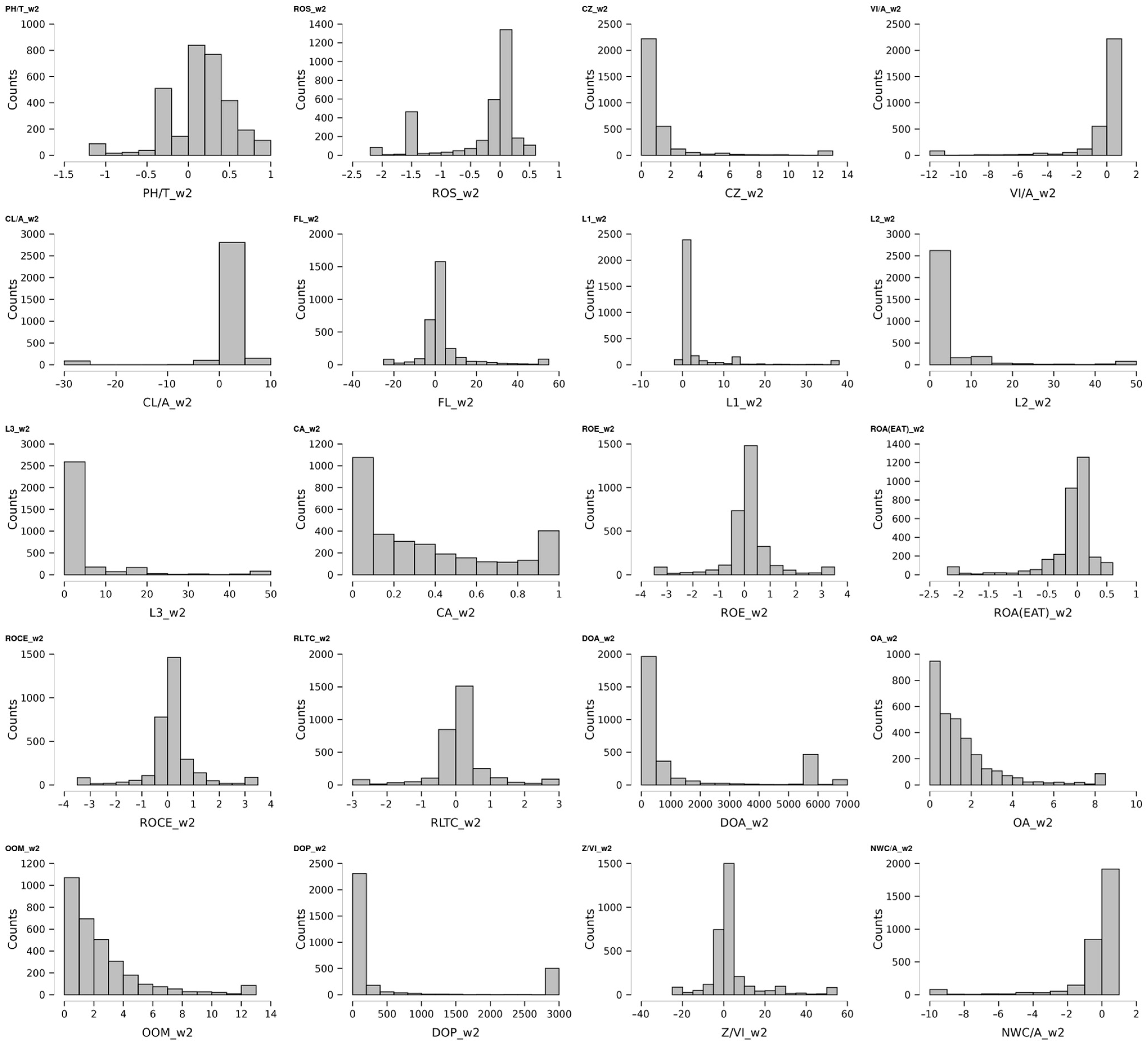
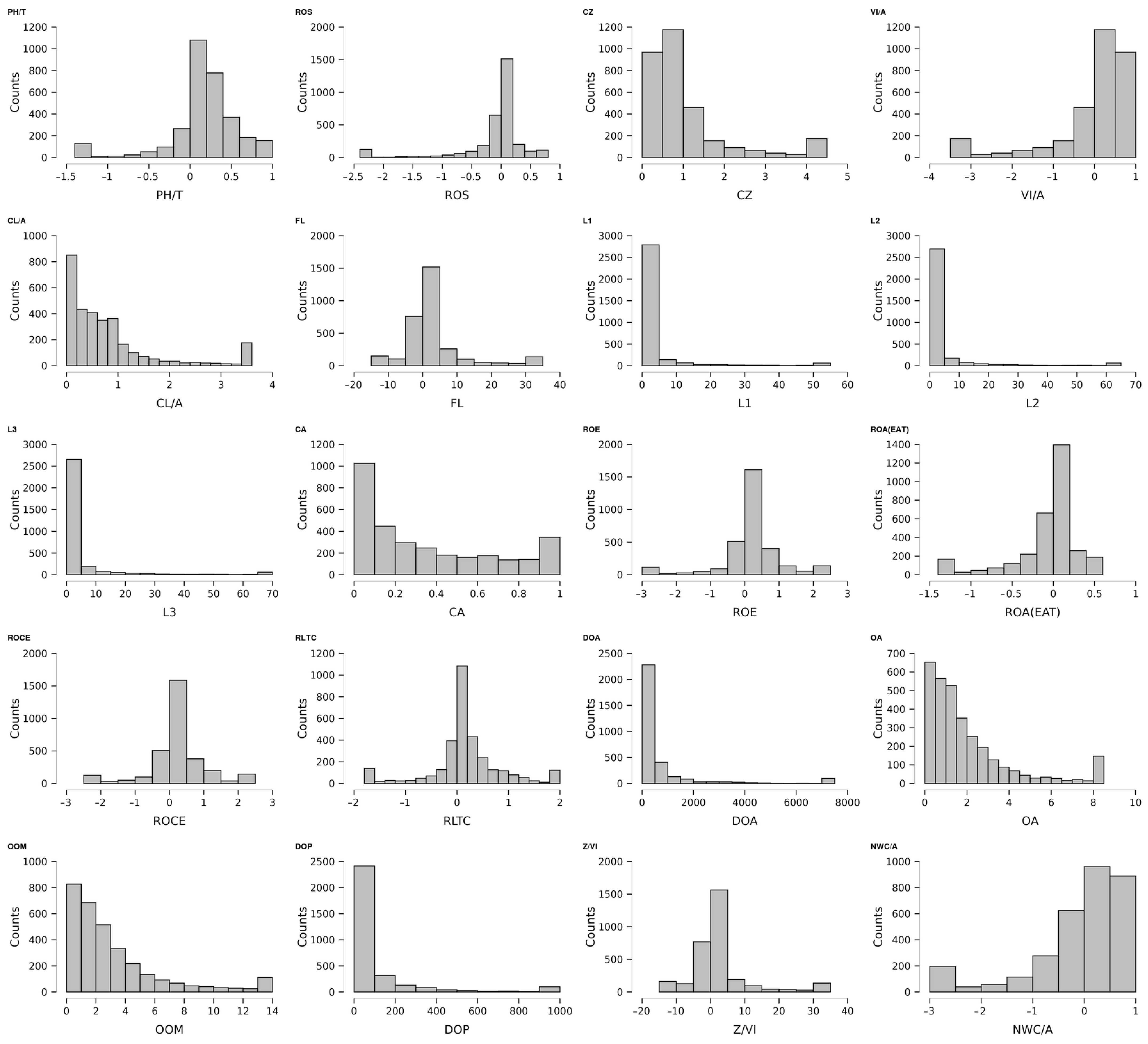
After preprocessing, the dataset was analyzed, and modeling was conducted using LR, SVMs, DTs, and ANNs. The descriptive statistics of the 2020 dataset are presented in

Table A1. Descriptive statistics of data (2020) before normalization.

	PH/T	ROS	CZ	VI/A	CL/A	FL	L1	L2	L3	CA	ROE	ROA	ROCE	RLTC	DOA	OA	OOM	DOP	Z/VI	NWC/A
Mean	0.126	−0.293	1.328	−0.329	0.244	3.638	2.924	4.028	4.311	0.352	0.135	−0.118	0.147	0.116	1431.012	1.558	2.443	569.68	3.165	−0.302
SE Mean	0.007	0.011	0.041	0.041	0.088	0.208	0.126	0.164	0.167	0.006	0.018	0.008	0.017	0.015	38.399	0.032	0.048	18.80	0.217	0.034
Std. Dev	0.413	0.641	2.303	2.302	4.932	11.671	7.059	9.207	9.370	0.340	1.030	0.468	0.968	0.821	2153.062	1.804	2.702	1054.5	12.155	1.890
IQR	0.391	0.422	0.764	0.762	0.792	3.899	1.335	2.054	2.181	0.538	0.383	0.184	0.388	0.314	931.813	1.679	2.682	204.1	4.291	0.867
Variance	0.170	0.411	5.302	5.301	24.328	136.206	49.833	84.766	87.797	0.115	1.061	0.219	0.936	0.674	4.6 × 10+6	3.255	7.302	1.1 × 10+6	147.74	3.571
Skewness	−0.891	−1.351	3.814	−3.814	−4.304	2.249	3.450	3.704	3.639	0.750	−0.275	−2.699	−0.132	−0.108	1.508	2.123	1.915	1.738	2.036	−3.551
SE Skew.	0.044	0.044	0.044	0.044	0.044	0.044	0.044	0.044	0.044	0.044	0.044	0.044	0.044	0.044	0.044	0.044	0.044	0.044	0.044	0.044
Kurtosis	1.263	0.560	14.904	14.903	22.369	7.511	12.143	14.148	13.670	−0.822	5.425	8.406	5.354	5.071	0.487	4.917	3.914	1.134	5.903	13.340
SE Kurt.	0.087	0.087	0.087	0.087	0.087	0.087	0.087	0.087	0.087	0.087	0.087	0.087	0.087	0.087	0.087	0.087	0.087	0.087	0.087	0.087
Range	2.063	2.627	12.705	12.705	36.566	72.752	36.272	49.156	49.720	1.000	6.966	2.667	6.554	5.506	6762.849	8.465	12.358	2939.1	72.658	10.433
Min.	−1.198	−2.123	0.000	−11.705	−26.679	−20.673	−1.8 × 10−5	0.003	0.005	5.15 × 10−5	−3.483	−2.115	−3.199	−2.713	38.991	0.000	0.000	0.000	−21.579	−9.433
Max.	0.866	0.504	12.705	1.000	9.887	52.079	36.272	49.160	49.724	1.000	3.483	0.552	3.355	2.792	6801.840	8.465	12.358	2939.1	51.079	1.000

and

Table A2. Descriptive statistics of data (2020) after preprocessing.

	PH/T	ROS	CZ	VI/A	CL/A	FL	L1	L2	L3	CA	ROE	ROA	ROCE	RLTC	DOA	OA	OOM	DOP	Z/VI	NWC/A
Mean	0.641	0.698	0.105	0.895	0.740	0.333	0.081	0.083	0.087	0.353	0.522	0.750	0.512	0.515	0.204	0.186	0.199	0.191	0.340	0.875
Std. Dev.	0.199	0.243	0.181	0.181	0.125	0.160	0.196	0.189	0.190	0.341	0.148	0.172	0.149	0.151	0.317	0.214	0.219	0.356	0.167	0.180
IQR	0.188	0.152	0.060	0.060	0.022	0.054	0.036	0.042	0.045	0.540	0.055	0.068	0.059	0.057	0.138	0.203	0.218	0.068	0.060	0.084
Variance	0.040	0.059	0.033	0.033	0.016	0.026	0.038	0.036	0.036	0.116	0.022	0.030	0.022	0.023	0.101	0.046	0.048	0.127	0.028	0.032
Skewness	−0.903	−1.377	3.827	−3.827	−4.561	2.268	3.441	3.686	3.627	0.748	−0.134	−2.743	−0.094	−0.062	1.523	2.090	1.891	1.763	2.050	−3.573
SE Skew.	0.047	0.047	0.047	0.047	0.047	0.047	0.047	0.047	0.047	0.047	0.047	0.047	0.047	0.047	0.047	0.047	0.047	0.047	0.047	0.047
Kurtosis	1.290	0.645	15.011	15.010	26.486	7.657	12.011	13.943	13.506	−0.838	5.397	8.783	5.266	5.007	0.539	4.745	3.788	1.228	6.001	13.562
SE Kurt.	0.093	0.093	0.093	0.093	0.093	0.093	0.093	0.093	0.093	0.093	0.093	0.093	0.093	0.093	0.093	0.093	0.093	0.093	0.093	0.093
Range	1.000	1.000	1.000	1.000	1.000	1.000	1.000	1.000	1.000	1.000	1.000	1.000	1.000	1.000	1.000	1.000	1.000	1.000	1.000	1.000
Min.	0.000	0.000	0.000	0.000	0.000	0.000	0.000	0.000	0.000	0.000	0.000	0.000	0.000	0.000	0.000	0.000	0.000	0.000	0.000	0.000
Max.	1.000	1.000	1.000	1.000	1.000	1.000	1.000	1.000	1.000	1.000	1.000	1.000	1.000	1.000	1.000	1.000	1.000	1.000	1.000	1.000

(Appendix A), while Figure A1 (Appendix B) illustrates the distribution density of individual indicators. The descriptive statistics for the 2022 dataset are provided in

Table A3. Descriptive statistics of data (2022) before normalization.

	PH/T	ROS	CZ	VI/A	CL/A	FL	L1	L2	L3	CA	ROE	ROA	ROCE	RLTC	DOA	OA	OOM	DOP	Z/VI	NWC/A
Mean	0.160	−0.108	1.037	−0.035	0.808	3.128	2.961	4.036	4.451	0.351	0.161	−0.080	0.190	0.146	751.063	1.991	3.145	107.477	2.116	−0.088
SE Mean	0.008	0.010	0.018	0.018	0.016	0.158	0.156	0.191	0.200	0.006	0.015	0.007	0.014	0.012	25.991	0.036	0.057	3.506	0.158	0.017
Std. Dev	0.426	0.549	1.010	1.006	0.902	8.892	8.743	10.740	11.239	0.330	0.858	0.410	0.813	0.688	1460.612	2.050	3.230	197.020	8.859	0.952
IQR	0.333	0.180	0.798	0.798	0.800	4.139	1.128	1.754	1.898	0.544	0.465	0.210	0.481	0.407	428.078	1.919	3.079	83.308	4.137	0.944
Variance	0.181	0.302	1.020	1.012	0.813	79.061	76.448	115.347	126.305	0.109	0.736	0.168	0.662	0.473	2.13 × 10+6	4.202	10.433	38,816.7	78.483	0.907
Skewness	−1.443	−2.477	1.777	−1.765	1.819	1.873	4.482	4.316	4.237	0.727	−1.065	−1.666	−0.681	−0.395	3.555	1.790	1.773	3.111	1.882	−1.460
SE Skew.	0.044	0.044	0.044	0.044	0.044	0.044	0.044	0.044	0.044	0.044	0.044	0.044	0.044	0.044	0.044	0.044	0.044	0.044	0.044	0.044
Kurtosis	3.595	6.897	2.700	2.653	2.721	4.379	20.707	19.200	18.530	−0.848	3.713	3.116	2.744	2.066	12.503	2.769	2.772	9.597	4.426	1.740
SE Kurt.	0.087	0.087	0.087	0.087	0.087	0.087	0.087	0.087	0.087	0.087	0.087	0.087	0.087	0.087	0.087	0.087	0.087	0.087	0.087	0.087
Range	2.203	2.953	4.064	4.038	3.523	45.310	52.393	63.390	65.999	0.999	4.740	1.966	4.386	3.589	7424.429	8.377	13.590	952.218	45.251	3.770
Min.	−1.276	−2.211	0.010	−3.048	0.005	−11.871	4.98 × 10−4	0.023	0.048	0.001	−2.737	−1.367	−2.343	−1.785	40.531	0.043	0.071	0.000	−12.841	−2.780
Max.	0.927	0.741	4.074	0.990	3.528	33.440	52.393	63.413	66.047	1.000	2.003	0.599	2.044	1.804	7464.960	8.420	13.661	952.218	32.410	0.989

and

Table A4. Descriptive statistics of data (2022) after preprocessing.

	PH/T	ROS	CZ	VI/A	CL/A	FL	L1	L2	L3	CA	ROE	ROA	ROCE	RLTC	DOA	OA	OOM	DOP	Z/VI	NWC/A
Mean	0.652	0.713	0.253	0.746	0.228	0.331	0.057	0.063	0.067	0.350	0.611	0.654	0.577	0.538	0.096	0.233	0.226	0.113	0.331	0.714
Std. Dev	0.193	0.186	0.249	0.249	0.256	0.196	0.167	0.169	0.170	0.330	0.181	0.209	0.185	0.192	0.197	0.245	0.238	0.207	0.196	0.253
IQR	0.151	0.061	0.196	0.198	0.227	0.091	0.022	0.028	0.029	0.545	0.098	0.107	0.110	0.114	0.058	0.229	0.227	0.087	0.091	0.250
Variance	0.037	0.035	0.062	0.062	0.066	0.039	0.028	0.029	0.029	0.109	0.033	0.044	0.034	0.037	0.039	0.060	0.056	0.043	0.038	0.064
Skewness	−1.443	−2.477	1.777	−1.765	1.819	1.873	4.482	4.316	4.237	0.727	−1.065	−1.666	−0.681	−0.395	3.555	1.790	1.773	3.111	1.882	−1.460
SE Skew.	0.044	0.044	0.044	0.044	0.044	0.044	0.044	0.044	0.044	0.044	0.044	0.044	0.044	0.044	0.044	0.044	0.044	0.044	0.044	0.044
Kurtosis	3.595	6.897	2.700	2.653	2.721	4.379	20.707	19.200	18.530	−0.848	3.713	3.116	2.744	2.066	12.503	2.769	2.772	9.597	4.426	1.740
SE Kurt.	0.087	0.087	0.087	0.087	0.087	0.087	0.087	0.087	0.087	0.087	0.087	0.087	0.087	0.087	0.087	0.087	0.087	0.087	0.087	0.087
Range	1.000	1.000	1.000	1.000	1.000	1.000	1.000	1.000	1.000	1.000	1.000	1.000	1.000	1.000	1.000	1.000	1.000	1.000	1.000	1.000
Min.	0.000	0.000	0.000	0.000	0.000	0.000	0.000	0.000	0.000	0.000	0.000	0.000	0.000	0.000	0.000	0.000	0.000	0.000	0.000	0.000
Max.	1.000	1.000	1.000	1.000	1.000	1.000	1.000	1.000	1.000	1.000	1.000	1.000	1.000	1.000	1.000	1.000	1.000	1.000	1.000	1.000

(Appendix A), and Figure A2 (Appendix B) depicts their distribution densities. A correlation analysis was performed, and strongly correlated indicators were excluded to prevent multicollinearity. Due to strong correlations among several indicators, eight predictors were excluded from further analysis (CZ, L1, L2, ROS, FL, ROCE, RLTC, and OOM). CZ showed a high correlation with VI/A and, to a lesser extent, with NWC/A, and was therefore removed. Among the liquidity indicators L1, L2, and L3, only L3 was retained due to their strong mutual correlation. ROS was excluded because of its correlation with PH/T and ROA. Although DOA and DOP exhibited some correlation, it was not substantial enough to warrant exclusion at the outset. CL/A was moderately correlated with VI/A but remained acceptable for further analysis. FL was highly correlated with Z/VI and partly with ROE, leading to its removal. Similarly, ROCE and RLTC were strongly correlated with ROE, so only ROE was retained. OOM was excluded due to its high correlation with OA. DOA and DOP provided limited explanatory value and contained a large proportion of missing data, while PH/T and CL/A demonstrated low predictive power in empirical tests and were therefore omitted. Empirical experiments confirmed that VI/A, L3, CA, ROA, NWC/A, OA, ROE, and Z/VI possessed predictive potential. The final models utilized VI/A, L3, CA, ROA, and NWC/A, as these variables consistently produced stable and reliable predictions. Although OA, ROE, and Z/VI also exhibited predictive ability, their marginal contribution and lower stability led to their exclusion from the final models. Certain ratios, specifically FL and CZ, were omitted from the models also due to their direct involvement in the definition of bankruptcy. Although the literature identifies these variables as strong predictors (Gavurova et al., 2022; Michalkova & Ponisciakova, 2025; Jenčová et al., 2020; Letkovský et al., 2024), their inclusion posed a risk of bias, as they are fundamentally linked to the bankruptcy classification itself. To mitigate this issue and ensure a more robust prediction model, these ratios were excluded from the modeling process. Empirical experiments with these predictors did not result in any significant improvement in model performance. Moreover, given their correlation with CZ and VI/A, it was reasonable to retain only one of them. Similarly, the simultaneous inclusion of FL and CZ consistently led to the model identifying one of them as redundant, as their shared information content caused only one to contribute meaningfully to the prediction.

3.2. Methods

The LR model remains one of the most widely applied techniques in bankruptcy prediction (Papana & Spyridou, 2020; Tomczak & Staszkiewicz, 2020; Kuiziniene et al., 2022; Billios et al., 2024). Systematic studies by Alaka et al. (2018), Tomczak and Staszkiewicz (2020), Clement et al. (2022), and Kuiziniene et al. (2022) highlight LR as a dominant approach, alongside AI-based models such as ANNs, SVMs, and DTs. However, due to the scope of this study, other approaches—particularly ensemble techniques that have gained popularity in recent years—were not tested. ANNs, SVMs, and DTs are considered fundamental classification models in bankruptcy prediction research. We consider these models to be basic or foundational techniques, widely applied due to their interpretability, availability in standard software packages, and strong theoretical foundations. In contrast, methods such as RF and GA are more often used as optimization tools, as performance enhancers for basic models, or as components within hybrid systems. Furthermore, ensemble methods—including boosting and bagging—are regarded as extension techniques that aggregate multiple classifiers to increase prediction accuracy and reduce overfitting. While other methods also appear in the literature, they are less frequently applied, making them more challenging to implement and validate due to limited empirical guidance and less established performance benchmarks.

3.2.1. Logistic Regression (LR)

The aim of the LR method is to identify the most appropriate and well-fitting model that explains the relationship between the output (dependent variable) and a set of input independent variables (predictors), commonly referred to as covariates. The model approximates a linear relationship for a binary outcome, differing primarily in the choice of the parametric model and its underlying assumptions (Hosmer & Lemeshow, 2000). LR is a widely used classical statistical method for prediction. It is a fundamental statistical method when applied to binary classification (predicting one of two possibilities, such as bankruptcy/non-bankruptcy). LR discusses in detail (Hosmer & Lemeshow, 2000). It models the relationship between independent variables and a discrete dependent variable. The independent variables can be continuous, categorical, or discrete.

LR applies a logit transformation to the dependent variable, effectively predicting the logit of Y from the set of independent variables X. The logit represents the natural logarithm of the odds of the event occurring, that is, the ratio of the probability that Y = 1 to the probability that Y = 0. In multiple LR, we consider y as the dependent variable (bankruptcy), as well as a set of k independent interval variables, which can be denoted by the vector x = [x₁, x₂ … x_k]^T. In the case of nominal variables, it is necessary to use a surrogate encoding of these values. The resulting probability condition is P(Y = 1|x) = π(x), and the logit of multiple LR will be given by

$$g(x)=a+b_1{x}_1+b_2{x}_2+\dots +b_k{x}_k$$

(1)

where fitting the model assumes a vector of estimation coefficients b = [a, b₁, … b_k]^T and the LR model is

$$\pi (x)={\displaystyle \frac{e^{g(x)}}{1+e^{g(x)}}}$$

(2)

The probability equations for j = 1, 2,…, k can be expressed as follows

$${\displaystyle {\sum }_i^n\left[y_i-\pi (x_i)\right]}=0\hspace{1em}\mathrm{and}\hspace{1em}{\displaystyle {\sum }_i^n{x}_{ij}\left[y_i-\pi (x_i)\right]}=0$$

(3)

The dependent variable can be transformed into a continuous variable using the odds ratio:

$$\mathrm{logit}(\pi )=\ln \left({\displaystyle \frac{\pi }{1-\pi }}\right)$$

(4)

where π represents the probability that the event will occur, i.e., p(Y = 1|x), and 1 − π represents the probability that the event (bankruptcy) will not occur. LR transforms nonlinear relationships into a linear form and assumes a logistic probability distribution:

$$\ln \left({\displaystyle \frac{\pi }{1-\pi }}\right)=\ln \left[e^{\left(a+b_1{x}_1+b_2{x}_2+\dots +b_k{x}_k\right)}\right]=a+b_i$$

(5)

where π is the probability of the event, a is the intercept, b_i represents regression coefficients, and x_i represents predictors. LR predicts log-odds of the outcome (Formula (5)). This means each coefficient represents the effect of a unit change in the predictor on the log-odds of the event. The logistic function represents an exponential function:

$$p(Y=1)={\displaystyle \frac{1}{1+e^{-\left(a+b_1{x}_1+b_2{x}_2+\dots +b_k{x}_k\right)}}}={\displaystyle \frac{1}{1+e^{-z}}}$$

(6)

Unlike linear regression, which produces a continuous output, LR applies the logistic (sigmoid) function to transform a linear combination of predictors into a value between 0 and 1. This value represents the probability of the outcome being 1 (i.e., the company going bankrupt). LR assumes that the predictors are not highly correlated and that the sample size is sufficiently large. A classification threshold of 0.5 was used in this study as the optimal value for a balanced dataset; however, as noted by Brygała (2022), this cut-off may be adjusted to improve classification performance. The probability can be expressed as a function of the vector of explanatory variables and their corresponding coefficients (Formula (6)).

The logit is defined as the natural logarithm of the odds ratio between the probability of bankruptcy and the probability of non-bankruptcy. When both probabilities are equal (p = 0.5), the logit equals zero. A positive logit value indicates p > 0.5, whereas a negative value indicates p < 0.5 (Iscaro et al., 2022).

In empirical model development, a null model (one without regressors) is first estimated to establish a baseline likelihood. Subsequently, the model including explanatory variables is tested using the likelihood ratio test. This test evaluates whether the inclusion of predictors significantly improves the model’s fit compared to the null model. The likelihood ratio statistic follows a chi-square distribution and can be calculated as

$${\chi }^2=-2\left(\ln L_0-\ln L_1\right)$$

(7)

where L₀ is the likelihood of the null model, and L₁ is the likelihood of the fitted model. A statistically significant result (p < 0.05) indicates that the fitted model performs better than the null model, confirming the appropriateness of applying logistic regression. Additionally, LR may incorporate regularization techniques to prevent overfitting (Máté et al., 2023).

3.2.2. Support Vector Machine (SVM)

The SVM method has been successfully applied in numerous studies on bankruptcy prediction (López Iturriaga & Sanz, 2015; Shin et al., 2005; Yoon & Kwon, 2010; Zhou et al., 2012; Barboza et al., 2017; Wei et al., 2024; Horak et al., 2020). The fundamental principle of SVMs is to identify hyperplanes in the feature space that maximize the separation between data points. Mathematically expressed separation of hyperplanes (Hamdi et al., 2024):

$$w\cdot x+b=0$$

(8)

where w is the vector of weighted coefficients, x is the input vector, and b is the bias. SVMs attempt to find the optimal values of w and b so that it constructs a hyperplane that best separates the two classes. The goal is not only to separate the classes, but also to maximize the margin, defined as the distance between the hyperplane and the nearest data points from each class (called support vectors). A larger margin indicates a clearer and more robust boundary, leading to better generalization on unseen data (Hamdi et al., 2024).

It is considered equivalent to quadratic optimization. One key advantage of SVMs is their ability to extract optimal decision boundaries even from small datasets, which is particularly beneficial in Slovakia, where prediction samples are often limited. Using support vectors, the SVM generates an estimation function for nonlinear class boundaries, with the support vectors representing the closest points to the optimal separation.

The SVM incorporates the principle of structural risk minimization, which enhances its generalization ability and makes it highly effective in pattern recognition. The SVM classification problem is formulated as a linearly constrained quadratic programming optimization task, in which support vectors are identified and the parameters w_i and b are estimated. Conceptually, SVM learning has some similarity to training a two-layer backpropagation neural network. However, rather than minimizing classification errors directly, SVMs maximize the margin between classes. This margin-based objective, derived from statistical learning theory, is designed to improve generalization performance, prioritizing robustness over simply fitting the training data (Shin et al., 2005).

It supports both classification and regression tasks and can handle continuous as well as categorical variables (Ptak-Chmielewska, 2019). A detailed discussion of SVM is provided in Vapnik (1995). For non-linear classification, SVMs employ the kernel trick, which replaces the standard dot product x_i^Tx_j with a kernel function K(x_i, x_j). This kernel implicitly maps the data into a higher-dimensional feature space, where linear separation becomes possible. The final SVM decision function is defined as (Vapnik, 19995):

$$f(x)=sign\left[{\displaystyle \sum _{i\in SV}{w}_i\cdot y_i\cdot K\left(x_i,x\right)+b}\right]$$

(9)

where the summation is performed only over support vectors (SV). This makes the model efficient and parsimonious, since only a subset of the training data contributes to the final classifier, y_i is the class label of the training example x_i, w_i are the learned weights, b is the bias term, and K(x_i, x) is the chosen kernel function.

3.2.3. Decision Tree (DT)

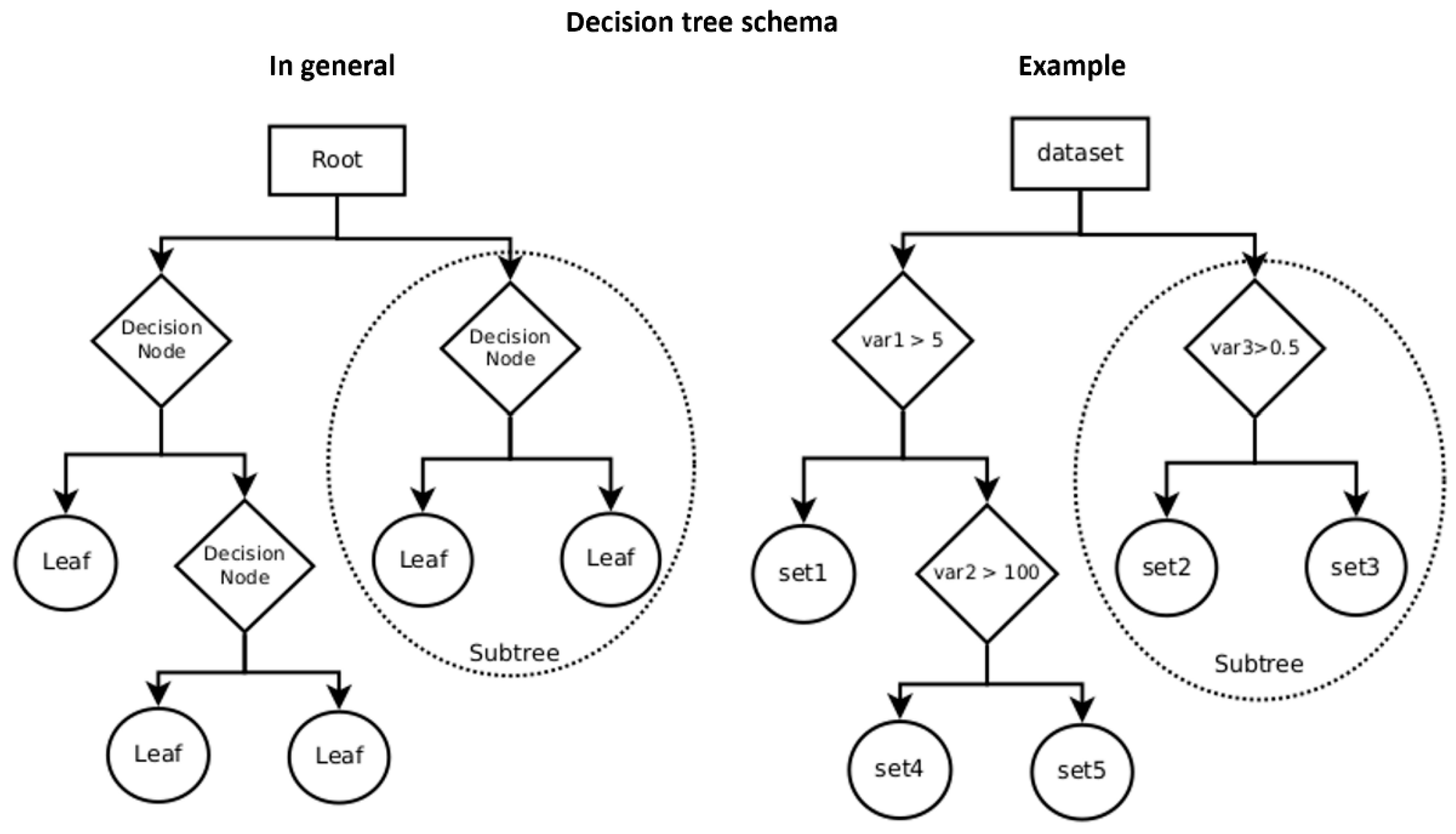
The DT method is based on the creation of decision rules that are hierarchically structured according to their importance. The process systematically segments the dataset into a tree-like structure. It begins with the entire dataset as the root, then applies rules to divide it into smaller subsets (nodes), and continues until reaching the leaves, which can no longer be split (Figure 2). Unlike regression-based models, DTs do not rely on coefficients or complex calculations during the process. However, like all ML methods, they are prone to overfitting.

The DT method constructs a model by creating a sequence of binary decision rules during the training to predict the class of a new sample. Each decision rule evaluates one of the independent input variables and splits the data into two groups based on that variable. This process continues recursively, forming branches of the tree. At the end of each branch (leaf node), a prediction of the output variable is assigned based on the majority class (for classification) or the average value (for regression) of the samples in that leaf. At each step, the algorithm selects the variable and split point that maximizes the separation of the data into internal homogeneous groups with respect to the output variable (Hamdi et al., 2024).

The key advantage of DTs is their transparent structure, which allows for easy interpretation of decision rules. They can handle both continuous and categorical variables. However, their primary drawback is a tendency to overfit, especially when trained on limited datasets. Additionally, DTs are sensitive to small variations in the data. The equation for training a decision tree can be written as (Máté et al., 2023):

$$h(x)=T(x,\theta ),$$

(10)

where h(x) is the prediction at certain points, represented by x; T forms the tree structure; and θ includes the parameters.

DTs create a set of rules that explain the relationship between dependent and independent variables. Their popularity has grown due to the simplicity with which the generated rules can be interpreted. DTs are particularly well-suited for variable selection, owing to their classification capabilities. The model works by dividing a heterogeneous group into smaller, more homogeneous subsets (Cho et al., 2010). For a decision tree (DT) to function effectively, a sufficiently large dataset with an adequate number of cases explaining the dependent variable is required. While outliers do not prevent the model’s use or validity, they can introduce distortions in the results. A DT does not rely on coefficients; instead, it is entirely based on partitioning rules that recursively split the dataset into groups. These rules are determined during the learning process and form the structure of the resulting model. The quality of each partition for a binary dependent variable is typically evaluated using Pearson’s χ² test, which measures the degree of association between the split and the outcome, and the Gini coefficient, which assesses the degree of impurity reduction achieved by the partition. A key advantage of DTs is their easy interpretability, as well as their robustness to missing data (Ptak-Chmielewska, 2019).

3.2.4. Artificial Neural Network (ANN)

The fundamental unit of an ANN is the artificial neuron, which functions similarly to a biological neuron. Its primary role is to aggregate input information using weight coefficients and transform this information into an output through an activation function. Various activation functions can be used, including sigmoid, hyperbolic tangent, softmax, linear, ReLU, and RBF. An innovative approach is the use of wavelets, as explored by Alexandridis and Zapranis (2013) and Lee and Su (2015). Neurons serve different functions, and by connecting identical neurons, layers are formed. These interconnected layers create a network. At a minimum, a network consists of two layers (input and output), but it can also include multiple hidden layers. The number of layers is not strictly predetermined; rather, it is a modeling decision. The number of input neurons corresponds to the number of input variables, while the number of output neurons depends on the classification task. In bankruptcy prediction, the output typically consists of either a single neuron with a value between 0 and 1 (indicating the probability of bankruptcy) or two neurons representing the classification classes (bankrupt/healthy). Although there is no strict limit on the maximum number of hidden nodes, Kolmogorov’s theorem suggests using 2n − 1 hidden neurons, where n represents the number of input variables.

The error in an ANN is typically quantified using the Root Mean Square Error (RMSE), which is a standard metric for measuring the difference between the predicted output and the actual values. RMSE represents the average magnitude of the error in the same units as the output variable, with lower values indicating better predictive performance. This metric is sensitive to outliers because it squares the differences between predicted and actual values. During training, the network iteratively adjusts the synaptic weights to minimize this error. Mathematically, RMSE can be expressed as:

$$RMSE=\sqrt{{\displaystyle \frac{1}{n}}{\displaystyle \sum _i{\left(y_i-{\widehat{y}}_i\right)}^2}},$$

(11)

where n is the number of samples, y_i is the actual value, and ${\widehat{y}}_i$ is the predicted value.

The most commonly used network types for prediction are multilayer perceptrons (MLP) with a feedforward (FF) structure and backpropagation (BP) learning. However, Igel and Hüsken (2003) found that the resilient propagation (RPROP) algorithm achieves better performance. López Iturriaga and Sanz (2015) highlight that ANNs do not require assumptions about data distribution, enabling them to establish complex relationships between predictors and dependent variables. ANNs offer high predictive performance, work well for both linear and nonlinear problems, and are relatively easy to implement (Aydin et al., 2022). Formally, the network can be represented as:

$$y=f\left({\displaystyle \sum _i{x}_i{w}_i}\right),$$

(12)

where y is the output, x_i are the inputs, w_i are the synaptic weights, and f is the activation function (

Table 3. Activation function.

Function	Graphic Representation	Equation
Linear		$f\left(x\right)=x$
H-tangent		$\tanh \left(x\right)={\displaystyle \frac{e^x-e^{-x}}{e^x+e^{-x}}}$
Step		$f\left(x\right)=\left[0,1\right]$
Treshold		$\theta \left(x\right)=x\theta \left(x\right)$
Sigmoid		$\sigma \left(x\right)={\displaystyle \frac{1}{1+e^{-x}}}$
RBF		$f\left(x\right)=e^{-x^2}$

).

3.2.5. Model Evaluation

The evaluation model was constructed using a confusion matrix, a 2 × 2 table that displays the classification frequencies of all cases in the sample. The primary metric for assessing classification performance is accuracy, which represents the proportion of correctly predicted cases. Its advantages include ease of implementation and interpretability.

Additional performance metrics include:

• Sensitivity (Recall)—the ratio of correctly predicted bankruptcies (true positives) to the total actual bankruptcies, measuring the model’s ability to identify bankrupt firms.
• Specificity—the ratio of correctly classified non-bankrupt firms (true negatives) to the total actual non-bankrupt firms, indicating the model’s effectiveness in detecting financially stable businesses.
• Precision—the ratio of correctly predicted bankruptcies (true positives) to all predicted bankruptcies, reflecting the reliability of bankruptcy classification.
  Mathematically, these metrics are expressed as follows:

  $$accuracy={\displaystyle \frac{TP+TN}{TP+TN+FP+FN}},$$

  (13)

  $$sensitivity={\displaystyle \frac{TP}{TP+FN}},$$

  (14)

  $$specificity={\displaystyle \frac{TN}{TN+FP}},$$

  (15)

  $$precision={\displaystyle \frac{TP}{TP+FP}},$$

  (16)

  where TP is True Positive, TN is True Negative, FP is False Positive, and FN is False Negative. To provide a more comprehensive comparison of the predictive performance across all models, this study utilizes the F-measure (specifically, the F1-score). The F-measure represents the harmonic means of precision and sensitivity (recall), offering a balanced evaluation of model performance. Its interpretation is straightforward and reliable, making it a robust metric, particularly when dealing with imbalanced datasets. Mathematically, the F-measure is expressed as:

  $$F\text{-}measure={\displaystyle \frac{2\cdot precision\cdot sensitivity}{precision+sensitivity}},$$

  (17)

When using LR, there is no direct equivalent to the R² statistic found in linear regression. Instead, pseudo-R² statistics are used to assess model fit. In this study, alternative measures of R² were applied to the LR model, specifically McFadden’s R², Nagelkerke’s R², and Cox and Snell’s R² indices. To achieve the goal of creating prediction models during the crisis and post-crisis period and comparing the accuracy of LR with AI-based models, the following approach was taken:

• Based on prior research, SVMs, DTs, and ANNs were selected as the most commonly used AI methods for comparison.
• The dataset was obtained from the Statistical Office of the Slovak Republic and Register of Financial Statements of the Slovak Republic databases.
• The year 2020 was chosen as the modeling period due to the unprecedented external economic disruptions, while 2022 represented the post-crisis period.
• Bankruptcy classification was conducted in accordance with Slovak legislation.
• Data preprocessing was performed prior to the analysis.
• Financial ratios were selected based on their prevalence in the literature and prior empirical studies.
• Modeling and evaluation were carried out.

The primary comparison of models was based on the F-measure, which balances precision and sensitivity. Additionally, a statistical test was conducted to evaluate the contribution of qualitative indicators to the LR model. This evaluation employed McFadden’s R² (McFadden, 1972), Nagelkerke’s R² (Nagelkerke, 1991), and Cox and Snell’s R² (Cox & Snell, 1989). Values approaching 1 (or 0.75) indicate a substantial improvement in model fit resulting from the inclusion of additional variables, whereas values close to zero suggest that the new model exhibits a similar fit to the baseline model—implying that the qualitative indicators had minimal or no effect on explanatory power.

Since there is no universally accepted method for selecting predictors, and the literature presents different approaches without a clear consensus, a pragmatic variable selection procedure was applied. First, a correlation analysis was performed, and only indicators that did not show strong mutual correlation were retained for the final model. To further verify the absence of multicollinearity, the Variance Inflation Factor (VIF) was calculated. While a VIF value below 10 is commonly regarded as acceptable, this study adopted a more conservative threshold of VIF < 4. This approach ensured that the selected variables were not excessively collinear, thereby enhancing the statistical robustness and interpretability of the model.

Additional techniques used for model evaluation included the Receiver Operating Characteristic (ROC) curve, which assesses the model’s performance in binary classification tasks. The ROC curve plots sensitivity (true positive rate) on the vertical axis against 1—specificity (false positive rate) on the horizontal axis. The Area Under the Curve (AUC) is a summary measure used to compare model performance, with values close to 1 indicating perfect classification and values near 0 representing complete misclassification. AUC is computed as the sum of the areas of trapezoidal segments formed between points of sensitivity and 1—specificity. This metric is scale-invariant, as it evaluates the model’s ranking ability rather than its absolute prediction values. Another commonly applied evaluation metric is the Gini index, which is derived from AUC of the ROC curve (Hand, 2009; Brown & Mues, 2012; Adeodato & Melo, 2022). It is widely used in credit scoring and bankruptcy prediction to assess the discriminatory power of classification models. Mathematically, the Gini index is calculated as:

$$Gini=2\cdot AUC-1.$$

(18)

The Gini index represents a linear transformation of the AUC and provides the same measure of classification performance on a different scale. A Gini value of 0 corresponds to a model with no discriminatory ability (i.e., random performance), whereas a value of 1 indicates perfect classification. Negative values suggest that the model performs worse than random guessing.

4. Results and Discussion

The selection of ML methods for comparison with the LR model was primarily based on the comparative study by Alaka et al. (2018), which found that ANNs, SVMs, and DTs performed similarly to LR. Their study also reported the frequency of use of various methods in the literature, showing that NN were the most frequently employed, followed by LR, SVM, multiple discriminant analysis (MDA), and DT. Another key source was du Jardin (2018), whose findings also indicated no statistically significant performance differences among basic classification methods. His work extended the comparison to ensemble and hybrid techniques. Although these advanced models often demonstrate superior predictive performance, they were not implemented in this study due to their higher requirements for model design, data processing, and computational complexity—factors that fall outside the intended scope of our research. Based on the popularity of the individual methods reported by the authors and summarized in Table 1, a statistical overview was created to identify the techniques most frequently used and those most often evaluated as the best-performing (see

Table 4. Frequency of use of prediction methods.

	DA	LR	SVM	DT	NN	RF	Specific
Summarized	13	24	16	15	27	9	21
As best-performing	1	2	3	3	8	2	17

). According to the frequency of use, NNs, LR, SVMs, and DTs emerged as the most applied methods, generally achieving the best results (when specific model variations are not considered). Consequently, these methods were selected for use in this study. While ensemble methods—by enhancing base learners through various optimization strategies—are considered highly promising, they are better categorized as advanced tools rather than basic classification methods. Similarly, hybrid models can be advantageous but involve substantial design and implementation complexity. For these reasons, the present study focuses exclusively on the comparison of basic methods, excluding ensemble and hybrid approaches.

The prediction results for all models are summarized in

Table 5. Prediction results of all models.

		LR		SVM		DT		ANN
	Only Financial	−	+	−	+	−	+	−	+
2020	Accuracy	0.840	0.844	0.840	0.851	0.880	0.858	0.893	0.884
	Sensitivity	0.834	0.848	0.840	0.851	0.880	0.858	0.893	0.884
	Specificity	0.860	0.840	0.839	0.851	0.880	0.854	0.893	0.883
	Precision	0.844	0.841	0.840	0.851	0.887	0.863	0.897	0.884
	F-measure	0.839	0.845	0.840	0.851	0.880	0.857	0.892	0.884
	AUC	0.820	0.831	0.839	0.851	0.880	0.854	0.895	0.883
	Gini	0.640	0.662	0.678	0.702	0.760	0.708	0.790	0.766
2022	Accuracy	0.865	0.861	0.882	0.870	0.866	0.872	0.898	0.891
	Sensitivity	0.863	0.867	0.882	0.870	0.866	0.872	0.898	0.891
	Specificity	0.867	0.855	0.882	0.870	0.866	0.874	0.898	0.890
	Precision	0.865	0.857	0.882	0.870	0.872	0.879	0.898	0.892
	F-measure	0.864	0.862	0.882	0.870	0.866	0.871	0.898	0.891
	AUC	0.877	0.877	0.882	0.870	0.866	0.874	0.897	0.885
	Gini	0.754	0.754	0.764	0.740	0.732	0.748	0.794	0.770

Note: LR—logistic regression; SVM—support vector machine; DT—decision tree; and ANN—artificial neural network. + denotes that only financial data has been used.

. For a comprehensive comparison, the F-measure metric was chosen, as it provides a more balanced assessment of model performance compared to accuracy. The results obtained from all applied methods were highly similar. One possible explanation is that the available data may not contain sufficient additional information to improve prediction accuracy without increasing the risk of overfitting. To better distinguish the performance of individual methods, a larger research sample, the inclusion of more—particularly qualitative—variables, or testing across different datasets (e.g., from different time periods, industries, or countries) would be necessary. Although LR achieved the lowest score in all cases, the difference was statistically very small. The comparable performance between LR and ML models suggests that LR is equally capable of capturing the relationship between financial indicators and the likelihood of bankruptcy. Another explanatory factor may be the use of identical input variables for all models, which may have limited each model abilities to fully leverage its unique strengths. While each method offers distinct methodological advantages, the aim of this study was to evaluate them under consistent conditions rather than to achieve optimal predictive accuracy.

Accuracy is a commonly used metric for evaluating model performance. However, its effectiveness diminishes considerably when applied to unbalanced datasets. Although the dataset in this study is balanced, the F-measure was chosen as the primary evaluation metric to enhance reliability. The F-measure considers both precision and recall, providing a more robust and informative indicator of predictive performance. The F-measure reflects the overall predictive ability and accuracy of the model. Additional metrics, such as accuracy, sensitivity, specificity, and precision, also serve as by-products of the evaluation process. Sensitivity helps determine Type I error (i.e., a bankrupt company incorrectly classified as healthy), while specificity helps determine Type II error (i.e., a healthy company incorrectly classified as bankrupt). The F-measure results of all models demonstrate strong predictive performance, confirming the validity of the modeling approach. A comparison of these models, presented in

Table 6. Comparison of model accuracy in studies from Slovakia and across the EU.

Author	Model	Accuracy [%]	F-Measure	AUC
Mihalovič (2018)	MDA	64.4	0.61
Mihalovič (2018)	NN	84.8	0.82
Mihalovič (2018)	GA-NN	91.2	0.89
Gregova et al. (2020)	LR			0.88
Gregova et al. (2020)	NN			0.89
Gregova et al. (2020)	RF			0.88
Jenčová et al. (2020)	LR	94.0	0.97	0.95
Horváthová et al. (2021)	MDA	83.3	0.91
Horváthová et al. (2021)	NN	97.2	0.97
Gavurova et al. (2022)	LR		0.94	0.9
Gavurova et al. (2022)	NN	99.8	1
Papík and Papíková (2023)	Boost (avg)	82.8		0.87
Letkovský et al. (2024)	LR	95.8	0.61	0.87
Letkovský et al. (2024)	NN, SVM, DT	96.1	0.96	0.75
Valaskova et al. (2023)	MDA	88.7	0.64
Horak et al. (2020)	SVM	76.1
Horak et al. (2020)	NN	82.8
Vochozka et al. (2020)	NN (LSTM)	89.8	0.93
Karas and Režňáková (2021)	MDA (avg)			0.75

, under similar conditions in Slovakia aligns with findings from previous studies (Horváthová et al., 2021; Papík & Papíková, 2023; Gregova et al., 2020; Gavurova et al., 2022; Tumpach et al., 2020; Jenčová et al., 2020; Letkovský et al., 2024; Brozyna et al., 2016; Mihalovič, 2018; Valaskova et al., 2023). Comparable research has also been conducted in the Czech Republic (Vochozka et al., 2020; Horak et al., 2020) and across the EU (Csikosova et al., 2019; Karas & Režňáková, 2021).

While the developed models demonstrate competitive predictive performance, direct comparisons are challenging due to variations in datasets and methodologies. For example, Jenčová et al. (2020) and Horváthová et al. (2021) focused on specific industries, enabling more precise differentiation between bankrupt and non-bankrupt companies, as financial data varies significantly across industries. Nonetheless, the models developed in this study could be applied in other EU countries with similar economic conditions, demonstrating their broader applicability and relevance.

Overall, the models exhibited a slight improvement in accuracy during the post-crisis period; however, this difference was not statistically significant. The comparison of model performance was conducted using the nonparametric McNemar test, which is designed to evaluate differences in paired nominal data within the same sample. The performance of DT, SVM, and ANN models was statistically compared to that of LR. The results of the McNemar test are presented in

Table 7. Comparison of performance metrics.

Models	Statistic	p-Value
LR—DT	92.6	0.0952
LR—SVM	41.0	0.7465
LR—ANN	62.3	0.2156
LR—DT (only financial ratio)	83.6	0.0863
LR—SVM (only financial ratio)	19.0	0.1189
LR—ANN (only financial ratio)	59.3	0.1092

. This observation can be partly explained by the increased sample size in the post-crisis dataset, which reflects the expanding number of enterprises within the Slovak industrial sector. The relative accuracy of the models suggests that no significant changes occurred during the crisis period that would render traditional prediction methods ineffective. While a slight decrease in accuracy is likely, this aligns with Papík and Papíková (2023), who demonstrated that economic crises negatively impact model accuracy compared to pre-crisis periods. However, the present study did not specifically quantify the magnitude of this effect due to its scope.

The primary objective was to determine whether bankruptcy prediction remains feasible during a crisis period using similar methods and to evaluate whether the LR model continues to perform comparably to AI-based techniques under such conditions.

The results indicate that all evaluated models exhibit relatively strong predictive performance, with only minor differences in their effectiveness. When only financial indicators were used, the LR model recorded the lowest F-measure, with values of 0.845 in 2020 and 0.862 in 2022. After the inclusion of qualitative indicators, achieving an F-measure of 0.839 in 2020 and 0.864 in 2022; however, the variation across models remained minimal. The highest predictive performance was observed for the ANN, which reached an F-measure of 0.892 (2020) and 0.898 (2022). In both cases, the LR model recorded the lowest performance among models using all available indicators, though the differences were not significant. Overall, ML models—specifically SVMs, DTs, and ANNs—outperformed the classical LR model in terms of predictive accuracy. When the predictions were repeated without including additional variables such as company size, the results were largely comparable. An interesting phenomenon can be observed in the slight increase in accuracy following the inclusion of the firm size variable in the LR and SVM models, accompanied by a decrease in accuracy in the DT and NN models in 2020. In the post-crisis period (2022), this relationship was reversed, with a decline in accuracy in the LR and SVM models and an improvement in the DT and NN models. However, these differences cannot be considered statistically significant. This reversal may indicate that the importance of firm size as a predictive variable changed between the crisis and post-crisis periods. During the crisis, firm size could have acted as a stabilizing factor, improving the performance of linear models such as LR and SVMs, whereas in the post-crisis environment, non-linear models like DTs and NNs may have been better able to capture the more complex relationships between firm size and financial distress. Although a slight decrease in accuracy was observed, the difference was negligible, suggesting that these variables did not significantly enhance predictive performance. The relative importance of individual predictors in the DT model is presented in

Table 8. Relative importance of features and multicollinearity diagnostics.

	2020			2022
Variable	Relative Importance	Tolerance	VIF	Relative Importance	Tolerance	VIF
VI/A	37.440	0.469	2.134	37.307	0.547	1.828
L3	21.268	0.707	1.415	21.879	0.797	1.255
CA	21.108	0.525	1.904	21.599	0.590	1.694
ROA	11.276	0.937	1.067	14.165	0.899	1.112
NWC/A	6.421	0.445	2.247	2.945	0.530	1.885
size	2.488	0.634	1.570	2.104	0.643	1.555

.

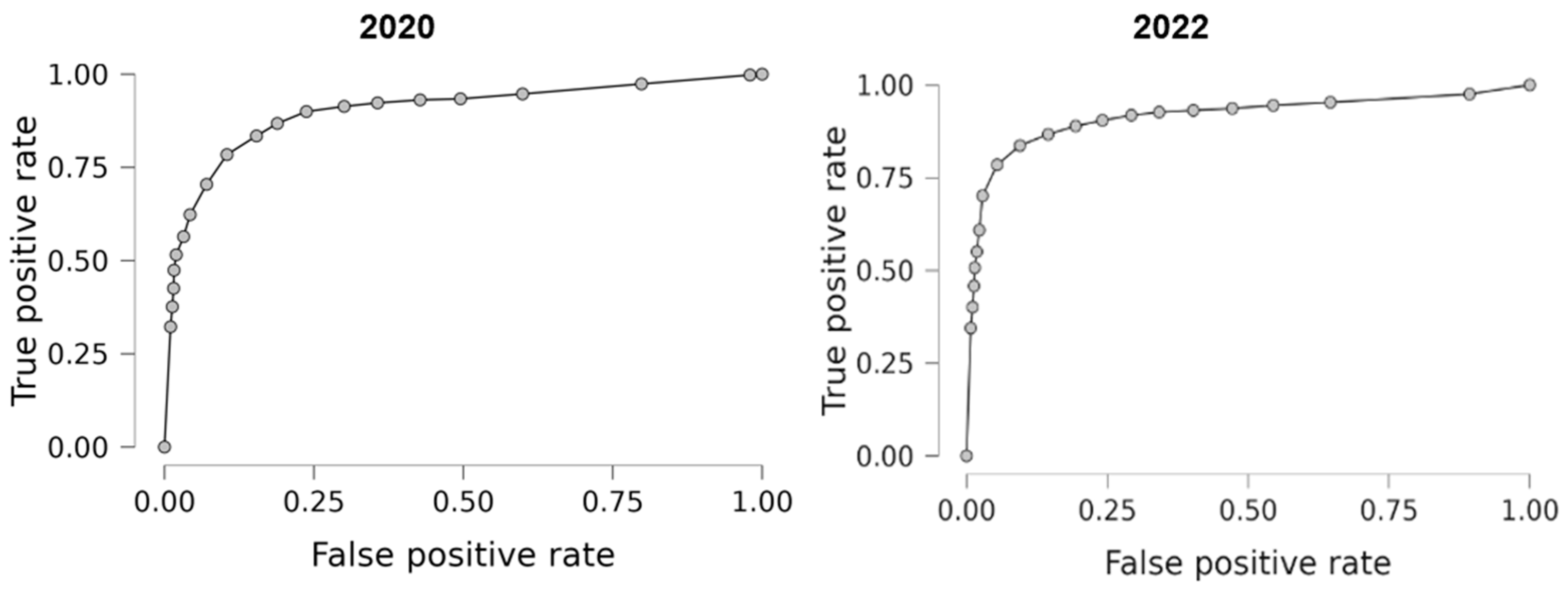
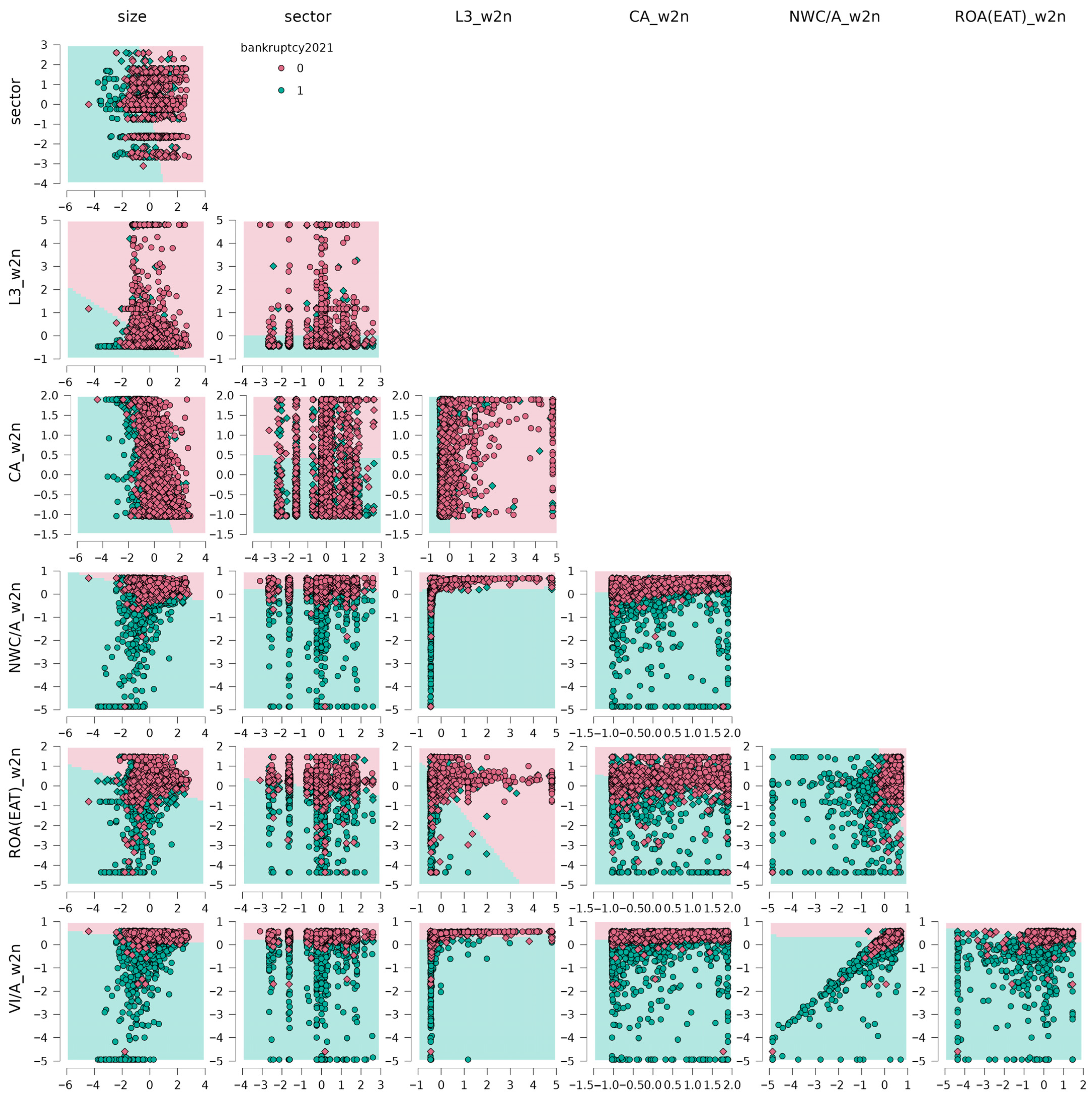
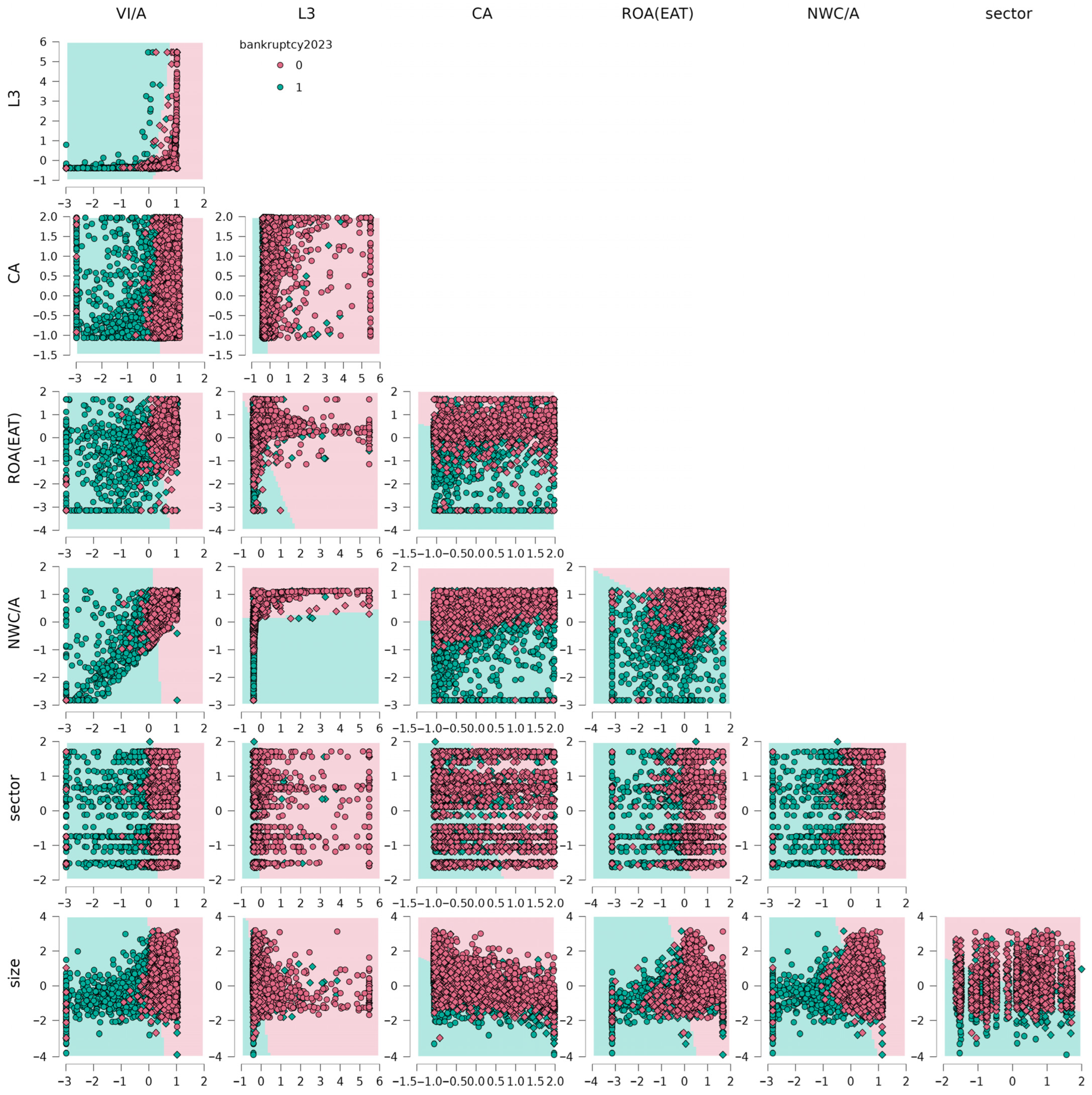
The analysis reveals that the company size is the least significant predictor, contributing to only 2%. In the LR model, size is identified as a significant variable (p < 0.001), with a negative effect on the dependent variable. This finding aligns with the study by Papík and Papíková (2023), which also demonstrated that adding categorical non-financial variables did not enhance prediction accuracy significantly. A possible explanation is that only SMEs were included in the dataset, and these enterprises operate under similar conditions in Slovakia. Consequently, these non-financial variables do not provide meaningful information for bankruptcy prediction. To quantify the impact of this factor, the statistics in

Table 9. Model summary of importance of nonfinancial predictors.

Year	Model	Deviance	AIC	BIC	df	χ2	p	McFadden R2	Nagelkerke R2	Cox and Snell R2
2020	M0	2415.882	2427.882	2463.406	2748			0.000	0.000	0.000
	M1	2371.863	2385.863	2427.309	2747	44.019	<0.001	0.018	0.027	0.016
2022	M0	2467.819	2479.819	2516.139	3138			0.000	0.000	0.000
	M1	2411.655	2425.655	2468.028	3137	56.164	<0.001	0.023	0.033	0.018

Note: Null model contains nuisance parameters: VI/A, L3, CA, ROA, NWC/A.

were calculated, comparing a model without company size (M₀) to a model including it (M₁). The low values of McFadden R², Nagelkerke R², and Cox and Snell R² confirm that the model incorporating this predictor provides only a negligible improvement over the null model. The LR coefficients are presented in

Table 10. Logistic regression coefficients.

							Wald Test			95% Conf. Inter.
Year	Model		Estimate	Std. Error	Odds Ratio	z	Wald Statistic	df	p	Lower	Upper
2020	M0	(Intercept)	44.471	2.146	2.059 × 10+19	20.719	429.287	1	<0.001	40.264	48.678
		VI/A	−42.786	2.691	2.621 × 10−19	−15.897	252.708	1	<0.001	−48.061	−37.510
		L3	−0.080	0.391	0.923	−0.204	0.042	1	0.838	−0.846	0.686
		CA	−0.202	0.220	0.817	−0.919	0.844	1	0.358	−0.632	0.229
		ROA	−2.359	0.563	0.095	−4.190	17.559	1	<0.001	−3.463	−1.256
		NWC/A	−0.068	1.676	0.934	−0.041	0.002	1	0.967	−3.353	3.216
		size	−0.459	0.070	0.632	−6.538	42.748	1	<0.001	−0.596	−0.321
	M2	(Intercept)	45.117	1.961	3.926 × 10+19	23.004	529.184	1	<0.001	41.273	48.961
		VI/A	−43.787	1.974	9.625 × 10−20	−22.186	492.231	1	<0.001	−47.656	−39.919
		ROA	−2.378	0.562	0.093	−4.230	17.892	1	<0.001	−3.480	−1.276
		size	−0.423	0.061	0.655	−6.980	48.716	1	<0.001	−0.542	−0.304
2022	M0	(Intercept)	17.533	0.765	4.115 × 10+7	22.933	525.902	1	<0.001	16.034	19.031
		VI/A	−16.271	0.899	8.578 × 10−8	−18.107	327.875	1	<0.001	−18.033	−14.510
		L3	0.522	0.449	1.686	1.164	1.356	1	0.244	−0.357	1.402
		CA	−0.677	0.222	0.508	−3.048	9.289	1	0.002	−1.112	−0.242
		ROA	−1.115	0.457	0.328	−2.441	5.958	1	0.015	−2.011	−0.220
		NWC/A	−0.753	0.593	0.471	−1.269	1.611	1	0.204	−1.916	0.410
		size	−0.595	0.081	0.552	−7.329	53.711	1	<0.001	−0.754	−0.436
	M2	(Intercept)	17.365	0.742	3.480 × 10+7	23.398	547.460	1	<0.001	15.910	18.820
		VI/A	−16.640	0.732	5.932 × 10−8	−22.739	517.076	1	<0.001	−18.075	−15.206
		CA	−0.734	0.212	0.480	−3.464	12.000	1	<0.001	−1.149	−0.319
		ROA	−1.145	0.457	0.318	−2.507	6.283	1	0.012	−2.041	−0.250
		size	−0.606	0.081	0.546	−7.505	56.327	1	<0.001	−0.764	−0.448

, and the ROC curves illustrating models’ performance are shown in Figure 3. The LR model labeled M₀ includes all five selected (uncorrelated) financial indicators, together with a non-financial variable (company size). Based on the Wald test, which indicated that some predictors contributed minimally to the model (i.e., exhibited high p-values), a reduced model labeled M₂ was developed. Model M₂ retains only the three (2020) and four (2022) most significant predictors: company size, VI/A, ROA in 2020, and CA in 2022. The reduction process followed the backward stepwise elimination method, in which variables are systematically removed to optimize model simplicity without compromising predictive power. The model verification statistics presented in

Table 11. Model summary for reduced predictor importance.

Year	Model	Deviance	AIC	BIC	df	χ2	p	McFadden R2	Nagelkerke R2	Cox and Snell R2
2020	M0	2371.179	2379.179	2402.863	2750			0.000	0.000	0.000
	M2	2371.863	2385.863	2427.309	2747	0.000		0.000	0.000	0.000
2022	M0	2414.088	2424.088	2454.354	3139			0.000	0.000	0.000
	M2	2411.655	2425.655	2468.028	3137	2.433	0.296	0.001	0.001	7.736 × 10−4

Note: Null model contains nuisance parameters: VI/A, ROA, size (2020) and VI/A, CA, ROA, size (2022).

—including McFadden R², Nagelkerke R², and Cox and Snell R²—show values close to zero, confirming that the reduced model performs comparably to the full model. Furthermore, the predictive accuracy of the LR model using M₂ remained largely unchanged, supporting the conclusion that the excluded indicators did not significantly improve or decrease model performance. Similarly, for the SVM model, the decision boundary matrix across all predictors is shown in Figure A3 for 2020 and Figure A4 for 2022 in Appendix C. Stepwise selection is generally discouraged in ML because it can lead to overfitting, relies on unstable statistical tests, ignores potential non-linear relationships between variables, and does not optimize predictive performance. Therefore, in this study, it was applied only to the LR model and not to ML methods.

Our analysis identified five key predictors that significantly contributed to bankruptcy prediction, achieving an accuracy level between 84% and 90%. Among these, VI/A emerged as one of the most influential indicators, with a relative importance of 37% according to the DT model. This metric reflects the extent of self-financing within a company and its capital structure, making it a strong predictor of financial stability. Its significance in bankruptcy prediction is supported by studies such as (Shin et al., 2005; Ptak-Chmielewska, 2019). VI/A also indirectly indicates indebtedness, providing complementary information to total debt levels. Given its close relationship with financial leverage, it would be valuable to exclude this predictor from the analysis to assess its impact on prediction accuracy. Liquidity predictors also played a crucial role, with the current ratio (L3) accounting for 21% of importance in the DT model. This differs from the LR model, where the indicator was found to be insignificant (p = 0.838 in 2020 and p = 0.244 in 2022). This ratio measures a company’s ability to promptly meet short-term obligations and reflects solvency. Its predictive relevance is consistent with findings of previous studies (Cheraghali & Molnár, 2025; Alexandridis & Zapranis, 2013; Nagelkerke, 1991; Cox & Snell, 1989). Similarly, NWC/A, which represents the proportion of working capital allocated to assets, contributed 21% to the prediction accuracy in the DT model. In the LR model, this indicator was marked as insignificant (p = 0.967 in 2020 and p = 0.204 in 2022). This metric highlights a company’s ability to cover short-term liabilities with available assets, an essential aspect of financial health. Its relevance in bankruptcy prediction has been previously demonstrated by several studies (Jabeur, 2017; Ogachi et al., 2020; Letkovský et al., 2024; Yousaf & Bris, 2021), with its importance tracking back to Altman’s seminal research (Altman, 1968). Another critical predictor, ROA, reflects the efficiency of asset utilization, indicating the proportion of profit generated relative to total assets. Its significance in bankruptcy prediction is intuitive, as a company that fails to generate sufficient returns from its assets is at a higher risk of financial instability. Insufficient profitability and a shortage of short-term assets can serve as early warning signals of impending failure. Finally, CA, which measures liquidity relative to assets, also proved to be a strong predictor, in line with the findings of Korol (2020). However, this indicator was marked as insignificant or irrelevant across all models.

The LR model (M₂) indicates that all three predictors (size, VI/A, ROA) have odds ratios lower than 1, suggesting a negative relationship with the likelihood of bankruptcy. Low value of odds ratio for company size confirms the well-established notion in the literature that firm size acts as a strong protective factor, as larger firms typically possess greater access to financing, higher diversification, and stronger market positions, which enhance their financial stability. The odds ratio for the equity-to-total-assets ratio (9.625 × 10⁻²⁰ in 2020 and 5.932 × 10⁻⁸ in 2022) indicates a strong negative relationship with bankruptcy likelihood. This suggests that firms with higher equity relative to their total assets are substantially less likely to go bankrupt. In economic terms, equity-rich firms have greater financial resilience and lower dependence on external debt, which significantly improves their solvency position. The odds ratio for the return on assets (ROA) variable was found to be 0.093 (or 0.318), depending on the model specification. In both cases, the value is below 1, which indicates a negative relationship between ROA and the likelihood of bankruptcy. This means that as profitability increases, the probability of bankruptcy decreases. Specifically, a one-unit increase in ROA reduces the odds of bankruptcy by approximately 90.7% when the odds ratio is 0.093 (2020), and by 68.2% when the odds ratio is 0.318 (2022). These results confirm that ROA is a strong protective indicator of financial health and stability. Firms with higher profitability are therefore significantly less likely to experience financial distress. The differences in the magnitude of the odds ratio across models may be attributed to variations in model specification, data structure, or the inclusion of other correlated indicators. Nonetheless, the consistent direction of the effect across models reinforces the importance of profitability as a determinant of bankruptcy risk. Similarly, the cash-to-assets ratio (CA) has an odds ratio of 0.48, meaning that a one-unit increase in liquidity corresponds to a 52% reduction in the odds of bankruptcy. This finding highlights the importance of liquidity in maintaining operational continuity and meeting short-term obligations. Overall, the results demonstrate that larger, more liquid firms with stronger asset-related financial ratios are significantly less likely to go bankrupt. These predictors, therefore, serve as important protective factors in bankruptcy prediction models.

According to the results obtained, although the set of predictors remained unchanged, their relative weights shifted slightly, which is a natural outcome. These predictors appear to be reliable and stable indicators, even during the crisis period. The prediction accuracy increased slightly in the post-crisis period, which is expected, as forecasting tends to be more accurate under stable economic conditions. This finding further supports the conclusion that bankruptcy is more predictable in non-crisis periods.

It is also likely that, thanks to government support measures, many SMEs managed to survive this unprecedented crisis period, whereas under normal circumstances, they might not have been able to. Consequently, when analyzing the data, we do not observe the dramatic structural changes in bankruptcy patterns that might have been expected. The impact of the pandemic seems to have spread out over time, thereby reducing its intensity. Of course, there is no doubt about the negative impact on businesses, as evidenced by the increased number of bankruptcies observed in the post-crisis period. This trend is partly attributable to the overall rise in the number of active entities.

Some studies have reported improvements in accuracy when applying the LASSO method, raising the question of whether alternative selection techniques could extract additional information and enhance model performance (e.g., Cheraghali & Molnár, 2025; Ozturkkal & Wahlstrøm, 2025; Pereira et al., 2016). Based on the results of the Wald statistic in the LR model, several indicators exhibited high p-values, indicating a limited contribution to the model’s explanatory power. Consequently, a hypothesis test was conducted to evaluate the effect of omitting the indicators L3, NWC/A, and CA in 2020. A likelihood ratio test comparing the reduced model, including only the indicators size, VI/A, and ROA in 2020, and CA in 2022—with the full model confirmed that the predictive accuracy remained virtually unchanged. Therefore, the LR model can be effectively applied using only these three key indicators.

The applied hyperparameters of the ML models were selected based on prior experience from previous research (Gavurova et al., 2022; Letkovský et al., 2024) and recommendations provided by other authors (Perez, 2006; Kim & Kang, 2010; Yoon & Kwon, 2010; López Iturriaga & Sanz, 2015; Thanh-Long & Hong-Chuong, 2022; Sigrist & Leuenberger, 2023). Subsequently, the final configuration was fine-tuned empirically. When training the DT, a minimum of 20 observations was required for node splitting, and at least 7 observations were required for terminal nodes. The maximum iteration depth was set to 30. The SVM algorithm was configured with a linear kernel function, a termination tolerance of 0.001, and an insensitive loss function parameter (epsilon) of 0.01. To control the trade-off between margin maximization and classification error, the regularization parameter C (cost of constraint violation) was fixed at 1. For the ANN model, an MLP with an FF architecture was used, as it is one of the most common NN structures in predictive modeling and has demonstrated strong performance. The optimal configuration included three nodes in the hidden layer, balancing model simplicity and predictive power. Empirical experiments demonstrated that increasing the number of nodes did not improve accuracy and instead led to overfitting. Likewise, varying the number of hidden layers had little effect on predictive performance, as networks with a single hidden layer achieved accuracy comparable to those with multiple layers. This finding aligns with observations by Gavurová et al. (Gavurova et al., 2022). The network architecture consisted of one input layer with seven nodes corresponding to the selected indicators and one output layer with a single node representing the binary classification (1 = bankrupt, 0 = healthy). The hyperbolic tangent function was used as the activation function. Although the BP learning algorithm is widely used in similar research (Shin et al., 2005; Tumpach et al., 2020; Thanh-Long & Hong-Chuong, 2022; Letkovský et al., 2024), the RPROP+ algorithm was employed in our study, as initial empirical experiments showed superior performance with this dataset. The effectiveness of different RPROP variants has been studied by Igel and Hüsken (2003), who identified iRPROP+ as the best-performing version. In this analysis, RPROP+ was preferred over BP due to its advantages in learning performance. Given the scope of the study, additional learning algorithms that might have marginally improved prediction accuracy were not explored in detail, although a general comparison of significance and accuracy was performed.

The issue of undetected bankruptcy probability can be partly attributed to the reduced quality of published financial data. The data used in this study were collected from publicly available financial statements, whose reliability may be limited due to both unintentional inaccuracies and deliberate manipulations by experienced financial managers (Mućko & Adamczyk, 2023). Furthermore, financial statement analyses are based on historical cost accounting and, therefore, disregard the time value of money. This methodological limitation further decreases data quality and, consequently, the reliability of predictive models. Additionally, the dataset contains missing values. While some missing data points can be estimated or imputed, such procedures inevitably introduce uncertainty. Excluding all observations with at least one missing value would, however, significantly reduce the sample size, particularly affecting the already limited number of bankrupt firms. This exclusion approach has been employed in studies such as (Hosaka, 2019; Gavurova et al., 2022; Andresson & Lukason, 2024; Letkovský et al., 2024), whereas others, including (Calabrese, 2023; López Iturriaga & Sanz, 2015; Wei et al., 2024; Pereira et al., 2016), opted for value imputation. To preserve an adequate sample quality, this study did not employ missing value imputation. Another challenge was the inability to adequately incorporate enterprise size as a variable. In most cases, data on the number of employees were either unavailable or outdated. As a result, firm size was approximated using total assets as a proxy variable. The potential benefits of incorporating qualitative data in bankruptcy prediction have been demonstrated by several studies (Karas & Režňáková, 2021; Korol & Fotiadis, 2022; Kaleem et al., 2024; Wei et al., 2024; Tobback et al., 2017; Arcuri & Levratto, 2020; Kwon & Lee, 2018; Asgarnezhad Nouri & Soltani, 2016). However, access to qualitative data remains a significant barrier in our context, as such data are available for only a limited number of firms. This limitation necessitates a primary focus on quantitative indicators. As a compromise, two qualitative variables—industry sector and firm size—were included. Nevertheless, sector affiliation demonstrated minimal explanatory power regarding the dependent variable. Given the categorical nature of the sector variables, the machine learning test revealed that it possessed virtually no explanatory power, and its contribution to the prediction performance was negligible or non-existent. Consequently, this variable was excluded from the subsequent models, as it was considered redundant and unnecessary for improving predictive accuracy. Firm size, when calculated using asset size, effectively becomes a quantitative measure, the quality of which remains low. If actual firm-level data (e.g., employee counts) were available, this variable would likely be of higher quality and could reduce uncertainty in the analysis; however, obtaining such information was not possible in our study. Furthermore, the usefulness of size and sector is constrained by the fact that the sample consists exclusively of SMEs, where variability in these characteristics is relatively small. A higher contribution of these variables could be expected if the dataset included large enterprises and corporations.

The application of a data reduction method presents both advantages and disadvantages. One of its principal benefits is the balancing of the dataset, which enables the models to focus more effectively on the minority class (bankrupt firms). The substantial reduction in dataset size also shortens the training time of machine learning models and lowers computational demands. Furthermore, redundant information arising from highly correlated observations may be partially eliminated. However, this approach also entails certain risks. The omission of samples may result in the loss of valuable information that reflects real-world conditions. Such information loss may reduce the model’s ability to generalize its learned patterns when applied to new data. Additionally, random selection may decrease the representativeness of the sample. This risk could be mitigated by employing more sophisticated, strategically designed sampling techniques rather than purely random selection methods.

Table 12. Key processing/modeling decisions.

n	Process	Sub-Process	Decision	Result
1	Data processing	Data collection	Company size, country, environment	Slovak SMEs–manufacturing
2			Period	Crisis (2020–2021), post-crisis (2022–2023) 1-year prediction
3		Feature selection	Financial ratio selection	Based on prior research, empirical experiments, availability = PH/T, ROS, CZ, VI/A, CL/A, FL, L1, L2, L3, CA, ROE, ROA, ROCE, RLTC, DOA, OA, OOM, DOP, Z/VI, NWC/A
4			Non-financial ratio selection	Company size
5			Multicollinearity	Strongly correlated ratio removed (CZ, L1, L2, ROS, FL, ROCE, RLTC, and OOM)
6		Preprocessing	Data consistency	Remove poor data completeness (lacking sufficient data)
7			Handle outliers	Winsorization (keep sample size) = 97.5th percentile, 2.5th percentile
8			Scaling	Normalization (0–1 range)
9			Balance	Under-sampling according to number of bankruptcy samples
10	Modeling		Select ML methods to compare LR	SVMs, DTs, ANNs
11			Dataset split for training	80:20 = random 80% for training
12			LR model	Cutoff point = 0.5, stepwise
13			SVM model	Linear kernel, termination 0.001, epsilon 0.01, fixed C = 1
14			DT model	Min. 20 observations for splitting, 7 for terminal, depth = 30
15			ANN model	MLP, FF, 1 hidden layer, 3–20 nodes, RPROP+
16	Model evaluation		Performance metrics	Accuracy, AUC, F-measure, Gini

presents a summary of important decisions in the research process.

5. Conclusions

Business risk assessment is an essential aspect of financial management, both for companies that need to continuously monitor their financial health to prevent crises and remain attractive to investors and for creditors who must make informed investment decisions. Different predictive methods are often comparable, making it essential not to rely on a single model but to validate predictions across multiple approaches to minimize the risk of misinterpretation.

The results indicate that effective predictive models can be developed using crisis-period data in a manner similar to standard periods. LR proves to be a reliable prediction method, maintaining comparable accuracy to AI techniques even during a crisis, without a significant decline in performance. This study focused on ML models—SVMs, NNs, and DTs—within the specific context of Slovakia, using a sample of SMEs during a period still influenced by the effects of COVID-19. The accuracy of these models was compared with LR, which, although a solid method, exhibited the lowest predictive accuracy. However, the differences between the models were not substantial enough to establish clear superiority. These findings suggest that ML models possess slightly higher potential for bankruptcy prediction than LR, though the difference in accuracy is modest, indicating room for further improvement. Given the scope of this study, not all ML approaches, such as RF or k-nearest neighbors (kNN), were explored.

The analysis did not reveal any distinct characteristics or vulnerabilities that could clearly indicate a forthcoming decline or provide management with an early warning to mitigate crisis impacts. Overall, the proposed models proved to be robust prediction tools, performing effectively not only under standard economic conditions but also during crisis periods.

One limitation of this study is the quality and scope of the dataset. The selection criteria included the number of employees, which many companies do not report, and a secondary criterion based on turnover or asset size. Additionally, only specific industries were included, limiting the applicability of the models to other sectors. Data quality is also a concern, as many companies fail to report even basic financial figures. The definition of bankruptcy used in the study serves as a theoretical framework but may not reflect actual business conditions; some companies meeting the defined criteria may continue operating and recover. Another limitation is the short two-year crisis period covered by the analysis, heavily influenced by the COVID-19 pandemic, as well as the two-year post-crisis period, which may make the results less representative of normal economic conditions.

Another limitation of this study concerns the configuration of the ML models. The hyperparameter search was conducted empirically, with parameter combinations selected according to their observed performance. Although this approach yielded satisfactory results, it does not guarantee identification of the global optimum. A more rigorous approach would involve a systematic exploration of the entire hyperparameter space (e.g., grid search or randomized search), which is computationally very demanding. Similarly, model validation was based on a single division of the dataset into training and testing subsets. For greater robustness and generalizability, multi-fold cross-validation would be preferable, as it repeatedly alternates validation subsets and produces an averaged performance estimate across multiple splits, thereby reducing the risk of sampling bias.

The selected crisis and immediate post-crisis period also represent an important limitation. The COVID-19 pandemic was an unprecedented economic shock, during which companies adopted extraordinary measures to ensure survival. Consequently, the quality and structure of publicly available financial data may have been more distorted than under normal market conditions. In addition, extensive state aid programs subsidized certain firms, temporarily preventing bankruptcies and altering natural market mechanisms. Such interventions may have weakened the relationship between financial distress indicators and actual bankruptcy events, potentially affecting the ability of the models to correctly identify distress patterns. In 2020, legislative measures (e.g., temporary moratoriums protecting debtors from bankruptcy proceedings) further influenced the observed outcomes. Moreover, external influences such as global market developments and foreign policy measures were not incorporated into the analysis, despite the fact that many companies operate internationally and are therefore directly or indirectly affected by cross-border economic conditions.

A major limitation of this study is the restricted access to qualitative data in the public conditions of the Slovak Republic. Financial indicators alone may not fully capture the true condition and prospects of companies. Prior research suggests that relying exclusively on financial variables may limit predictive performance, as the inclusion of qualitative information has been shown to enhance bankruptcy prediction accuracy. Future research should therefore consider incorporating additional variables such as the number of customers, order volumes, supplier relationships, management characteristics, and relevant macroeconomic indicators. A further limitation lies in the construction of the dataset through the application of random undersampling. While this approach helps to address class imbalance, it carries the risk of losing potentially valuable information and may not fully reflect real-world conditions. Future research should therefore consider more strategic sampling procedures or more sophisticated selection techniques, such as methods based on cluster centroids.

Additionally, the absence of verified information on the actual bankruptcy status of individual companies restricts the conclusions to a more theoretical level and limits the possibility of fully validating the predictive performance of the models.

Future research should apply the same methodology to different countries and industries, where higher-quality data may better reveal the real potential of ML in bankruptcy prediction. These results contribute to the literature by introducing AI-based models tailored to Slovakia’s SMEs and demonstrating that ML techniques provide high accuracy in bankruptcy estimation while maintaining stability compared with traditional statistical methods, such as LR.

One of the main contributions of this study is the development of bankruptcy detection models for SMEs in the Slovak industrial sector. These models have practical applications for financial managers and creditors and serve as valuable references for the academic community. The research further contributes through a comprehensive literature review on bankruptcy prediction and the implementation of the most frequently used methods within the context of Slovakia’s rapidly developing SME economy. Conducting this analysis during a period of economic crisis provides a meaningful benchmark for future comparisons in non-crisis conditions. From a scientific standpoint, examining models created during crisis periods is highly relevant, as key indicators may differ significantly from those observed in stable economic environments. This raises an important research question: do the key predictors identified during a crisis really differ from those in normal times? The study also contributes to the expansion of the knowledge base in financial management, with a notable aspect being the comparison of ML techniques with traditional LR. Both approaches yielded similarly strong results on the analyzed sample, supporting the view that LR remains a valid and effective prediction tool. These findings offer practitioners a practical and cost-efficient method to maintain competitiveness, enhance financial analysis, improve economic monitoring, and strengthen debt management.

This study focuses on two distinct periods: the crisis and the immediate post-crisis phase. By comparing predictive models under these specific conditions, the research contributes to a deeper understanding of bankruptcy detection across different economic environments. The sample analyzed originates from an economy predominantly composed of small and medium-sized enterprises, which may respond differently to crisis situations. On the one hand, SMEs tend to demonstrate greater flexibility and adaptability to rapidly changing conditions. On the other hand, they often lack sufficient capital resilience to withstand unexpected shocks. The study further contributes to the field of bankruptcy prediction by providing a literature review with a particular emphasis on SMEs, as well as empirical evidence on the application of LR and machine learning methods, achieving comparable levels of predictive accuracy. Moreover, it offers an empirical examination of the crisis period in the context of bankruptcy prediction and a subsequent comparison with the post-crisis period.

Future research should place greater emphasis on qualitative indicators and explore alternative sources of information beyond purely financial data. It would also be beneficial to expand the range of models to include additional ensemble techniques and to examine periods more distant from the crisis to assess the longer-term stability and robustness of predictive performance. Bankruptcy risk can be mitigated through proactive financial management, including careful monitoring of revenues and expenditures, increased operational efficiency, and effective communication with creditors. Furthermore, management is encouraged to draw upon research of this nature and to utilize predictive models as early warning tools for identifying potential financial difficulties at an early stage.

References

1. Addo, P. M., Guegan, D., & Hassani, B. (2018). Credit risk analysis using machine and deep learning models. Risks, 6(2), 38. [Google Scholar] [CrossRef]
2. Adeodato, P., & Melo, S. (2022, July 18–23). A geometric proof of the equivalence between AUC_ROC and Gini index area metrics for binary classifier performance assessment [Paper Presentation]. 2022 International Joint Conference on Neural Networks (IJCNN), Padua, Italy. [Google Scholar] [CrossRef]
3. Agarwal, A. (1999). Abductive networks for two-group classification: A comparison with neural networks. Journal of Applied Business Research (JABR), 15(2), 1–12. [Google Scholar] [CrossRef]
4. Alaka, H. A., Oyedele, L. O., Owolabi, H. A., Kumar, V., Ajayi, S. O., Akinade, O. O., & Bilal, M. (2018). Systematic review of bankruptcy prediction models: Towards a framework for tool selection. Expert Systems with Applications, 94, 164–184. [Google Scholar] [CrossRef]
5. Alexandridis, A. K., & Zapranis, A. D. (2013). Wavelet neural networks: A practical guide. Neural Networks, 42, 1–27. [Google Scholar] [CrossRef] [PubMed]
6. Altman, E. I. (1968). Financial ratios, discriminant analysis and the prediction of corporate bankruptcy. The Journal of Finance, 23, 589–609. [Google Scholar] [CrossRef]
7. Andresson, A., & Lukason, O. (2024). Corporate default prediction with payment disturbances in managers’ earlier entrepreneurial practices. Cogent Business & Management, 11(1), 2302203. [Google Scholar] [CrossRef]
8. Andrikopoulos, P., & Khorasgani, A. (2018). Predicting unlisted SMEs’ default: Incorporating market information on accounting-based models for improved accuracy. The British Accounting Review, 50(5), 559–573. [Google Scholar] [CrossRef]
9. Arcuri, G., & Levratto, N. (2020). Early stage SME bankruptcy: Does the local banking market matter? Small Business Economics, 54(2), 421–436. [Google Scholar] [CrossRef]
10. Asgarnezhad Nouri, B., & Soltani, M. (2016). Designing a bankruptcy prediction model based on account, market and macroeconomic variables (case study: Cyprus stock exchange). Iranian Journal of Management Studies, 9(1), 125–147. [Google Scholar]
11. Aydin, N., Sahin, N., Deveci, M., & Pamucar, D. (2022). Prediction of financial distress of companies with artificial neural networks and decision trees models. Machine Learning with Applications, 10, 100432. [Google Scholar] [CrossRef]
12. Bakhtiari, S., Breunig, R., Magnani, L., & Zhang, J. (2020). Financial constraints and small and medium enterprises: A review. Economic Record, 96(315), 506–523. [Google Scholar] [CrossRef]
13. Barboza, F., Kimura, H., & Altman, E. (2017). Machine learning models and bankruptcy prediction. Expert Systems with Applications, 83, 405–417. [Google Scholar] [CrossRef]
14. Beade, Á., Rodríguez, M., & Santos, J. (2024). Business failure prediction models with high and stable predictive power over time using genetic programming. Operational Research, 24(3), 52. [Google Scholar] [CrossRef]
15. Beaver, W. H. (1966). Financial ratios as predictors of failure. Journal of Accounting Research, 4, 71. [Google Scholar] [CrossRef]
16. Becerra-Vicario, R., Alaminos, D., Aranda, E., & Fernández-Gámez, M. A. (2020). Deep recurrent convolutional neural network for bankruptcy prediction: A case of the restaurant industry. Sustainability, 12(12), 5180. [Google Scholar] [CrossRef]
17. Belaid, F., Boussaada, R., & Belguith, H. (2017). Bank-firm relationship and credit risk: An analysis on Tunisian firms. Research in International Business and Finance, 42, 532–543. [Google Scholar] [CrossRef]
18. Billios, D., Seretidou, D., & Stavropoulos, A. (2024). The power of numerical indicators in predicting bankruptcy: A systematic review. Journal of Risk and Financial Management, 17(10), 433. [Google Scholar] [CrossRef]
19. Botsari, A., Gvetadze, S., & Lang, F. (2024). The European small business finance outlook 2024 (EIF Working Paper No. 2024/101). European Investment Fund (EIF). Available online: https://www.econstor.eu/bitstream/10419/313620/1/1919672362.pdf (accessed on 8 March 2026).
20. Brown, I., & Mues, C. (2012). An experimental comparison of classification algorithms for imbalanced credit scoring data sets. Expert Systems with Applications, 39(3), 3446–3453. [Google Scholar] [CrossRef]
21. Brozyna, J., Mentel, G., & Pisula, T. (2016). Statistical methods of the bankruptcy prediction in the logistics sector in Poland and Slovakia. Transformations in Business & Economics, 15(1), 93–114. [Google Scholar]
22. Brygała, M. (2022). Consumer bankruptcy prediction using balanced and imbalanced data. Risks, 10(2), 24. [Google Scholar] [CrossRef]
23. Calabrese, R. (2023). Contagion effects of UK small business failures: A spatial hierarchical autoregressive model for binary data. European Journal of Operational Research, 305(2), 989–997. [Google Scholar] [CrossRef]
24. Callejón, A. M., Casado, A. M., Fernández, M. A., & Peláez, J. I. (2013). A system of insolvency prediction for industrial companies using a financial alternative model with neural networks. International Journal of Computational Intelligence Systems, 6(1), 29–37. [Google Scholar] [CrossRef][Green Version]
25. Campa, D. (2015). The impact of SME’s pre-bankruptcy financial distress on earnings management tools. International Review of Financial Analysis, 42, 222–234. [Google Scholar] [CrossRef]
26. Chen, Y. S., Lin, C. K., Lo, C. M., Chen, S. F., & Liao, Q. J. (2021). Comparable studies of financial bankruptcy prediction using advanced hybrid intelligent classification models to provide early warning in the electronics industry. Mathematics, 9(20), 2622. [Google Scholar] [CrossRef]
27. Cheraghali, H., & Molnár, P. (2025). SME default prediction: A systematic methods evaluation. Journal of Small Business Management, 63(4), 1466–1517. [Google Scholar] [CrossRef]
28. Cho, S., Hong, H., & Ha, B. C. (2010). A hybrid approach based on the combination of variable selection using decision trees and case-based reasoning using the Mahalanobis distance: For bankruptcy prediction. Expert Systems with Applications, 37(4), 3482–3488. [Google Scholar] [CrossRef]
29. Clement, C., David, M., & Jemna, D. V. (2022). Bankruptcy prediction using machine learning—A meta-analysis. Journal of Public Administration, Finance and Law, 26, 63–77. [Google Scholar] [CrossRef]
30. Cowling, M., Brown, R., & Rocha, A. (2020). Did you save some cash for a rainy COVID-19 day? The crisis and SMEs. International Small Business Journal, 38(7), 593–604. [Google Scholar] [CrossRef] [PubMed]
31. Cox, D. R., & Snell, E. J. (1989). Analysis of binary data (2nd ed.). Chapman & Hall. [Google Scholar]
32. Csikosova, A., Janoskova, M., & Culkova, K. (2019). Limitation of financial health prediction in companies from post-communist countries. Journal of Risk and Financial Management, 12(1), 15. [Google Scholar] [CrossRef]
33. Dasilas, A., & Rigani, A. (2024). Machine learning techniques in bankruptcy prediction: A systematic literature review. Expert Systems with Applications, 255, 124761. [Google Scholar] [CrossRef]
34. Dhamo, Z., Gjeçi, A., Zibri, A., & Prendi, X. (2025). Business distress prediction in Albania: An analysis of classification methods. Journal of Risk and Financial Management, 18(3), 118. [Google Scholar] [CrossRef]
35. du Jardin, P. (2018). Failure pattern-based ensembles applied to bankruptcy forecasting. Decision Support Systems, 107, 64–77. [Google Scholar] [CrossRef]
36. Duricova, L., Kovalova, E., Gazdíková, J., & Hamranova, M. (2025). Refining the best-performing V4 financial distress prediction models: Coefficient re-estimation for crisis periods. Applied Sciences, 15(6), 2956. [Google Scholar] [CrossRef]
37. Eurostat. (2022). Business bankruptcy declarations—Quarterly data. European Commission. [Google Scholar]
38. Fasano, F., Adornetto, C., Zahid, I., La Rocca, M., Montaleone, L., Greco, G., & Cariola, A. (2024). The dilemma of accuracy in bankruptcy prediction: A new approach using explainable AI techniques to predict corporate crises. European Journal of Innovation Management, 28(11), 1–22. [Google Scholar] [CrossRef]
39. Fischer, T., & Krauss, C. (2018). Deep learning with long short-term memory networks for financial market predictions. European Journal of Operational Research, 270(2), 654–669. [Google Scholar] [CrossRef]
40. Fitzpatrick, P. J. (1932). A comparison of ratios of successful industrial enterprises with those of failed firm. Certified Public Accountant, 6, 727–731. [Google Scholar]
41. Garcia, J. (2022). Bankruptcy prediction using synthetic sampling. Machine Learning with Applications, 9, 100343. [Google Scholar] [CrossRef]
42. Gavurova, B., Jencova, S., Bačík, R., Miskufova, M., & Letkovský, S. (2022). Artificial intelligence in predicting the bankruptcy of non-financial corporations. Oeconomia Copernicana, 13(4), 1215–1251. [Google Scholar] [CrossRef]
43. Gregova, E., Valaskova, K., Adamko, P., Tumpach, M., & Jaros, J. (2020). Predicting financial distress of slovak enterprises: Comparison of selected traditional and learning algorithms methods. Sustainability, 12(10), 3954. [Google Scholar] [CrossRef]
44. Gupta, J., Gregoriou, A., & Healy, J. (2015). Forecasting bankruptcy for SMEs using hazard function: To what extent does size matter? Review of Quantitative Finance and Accounting, 45(4), 845–869. [Google Scholar] [CrossRef]
45. Hamdi, M., Mestiri, S., & Arbi, A. (2024). Artificial intelligence techniques for bankruptcy prediction of tunisian companies: An application of machine learning and deep learning-based models. Journal of Risk and Financial Management, 17(4), 132. [Google Scholar] [CrossRef]
46. Han, I., Chandler, J. S., & Liang, T. P. (1996). The impact of measurement scale and correlation structure on classification performance of inductive learning and statistical methods. Expert Systems with Applications, 10(2), 209–221. [Google Scholar] [CrossRef]
47. Hand, D. J. (2009). Measuring classifier performance: A coherent alternative to the area under the ROC curve. Machine Learning, 77(1), 103–123. [Google Scholar] [CrossRef]
48. Hanweck, G. (1977). Predicting bank failures (Research Papers in Banking and Financial Economics, 19). Board of Governors of the Federal Reserve System (U.S.). Available online: https://ideas.repec.org/p/fip/fedgbf/19.html (accessed on 8 March 2026).
49. Horak, J., Vrbka, J., & Suler, P. (2020). Support vector machine methods and artificial neural networks used for the development of bankruptcy prediction models and their comparison. Journal of Risk and Financial Management, 13(3), 60. [Google Scholar] [CrossRef]
50. Horváthová, J., Mokrišová, M., & Petruška, I. (2021). Selected methods of predicting financial health of companies: Neural networks versus discriminant analysis. Information, 12(12), 505. [Google Scholar] [CrossRef]
51. Hosaka, T. (2019). Bankruptcy prediction using imaged financial ratios and convolutional neural networks. Expert Systems with Applications, 117, 287–299. [Google Scholar] [CrossRef]
52. Hosmer, D. W., & Lemeshow, S. (2000). Applied logistic regression. John Wiley & Sons. [Google Scholar]
53. Huo, Y., Chan, L. H., & Miller, D. (2024). Bankruptcy prediction for restaurant firms: A comparative analysis of multiple discriminant analysis and logistic regression. Journal of Risk and Financial Management, 17(9), 399. [Google Scholar] [CrossRef]
54. Igel, C., & Hüsken, M. (2003). Empirical evaluation of the improved Rprop learning algorithms. Neurocomputing, 50, 105–123. [Google Scholar] [CrossRef]
55. Iscaro, V., Castaldi, L., Maresca, P., & Mazzoni, C. (2022). Digital transformation in the economics of complexity: The role of predictive models in strategic management. Journal of Strategy and Management, 15(3), 450–467. [Google Scholar] [CrossRef]
56. Jabeur, S. B. (2017). Bankruptcy prediction using partial least squares logistic regression. Journal of Retailing and Consumer Services, 36, 197–202. [Google Scholar] [CrossRef]
57. Jenčová, S., Štefko, R., & Vašaničová, P. (2020). Scoring model of the financial health of the electrical engineering industry’s non-financial corporations. Energies, 13(17), 4364. [Google Scholar] [CrossRef]
58. Kaleem, M., Raza, H., Ashraf, S., Almeida, A. M., & Machado, L. P. (2024). Does ESG predict business failure in Brazil? An application of machine learning techniques. Risks, 12(12), 185. [Google Scholar] [CrossRef]
59. Karas, M. (2017). The stability of bankruptcy predictors in the construction and manufacturing industries at various times before bankruptcy. E+M Economics and Management, 20(2), 116–133. [Google Scholar] [CrossRef]
60. Karas, M., & Režňáková, M. (2021). The role of financial constraint factors in predicting SME default. Equilibrium. Quarterly Journal of Economics and Economic Policy, 16(4), 859–883. [Google Scholar] [CrossRef]
61. Khashei, M., Etemadi, S., & Bakhtiarvand, N. (2024). A new discrete learning-based logistic regression classifier for Bankruptcy prediction. Wireless Personal Communications, 134(2), 1075–1092. [Google Scholar] [CrossRef]
62. Kim, M. J., & Kang, D. K. (2010). Ensemble with neural networks for bankruptcy prediction. Expert Systems with Applications, 37(4), 3373–3379. [Google Scholar] [CrossRef]
63. Kitowski, J., Kowal-Pawul, A., & Lichota, W. (2022). Identifying symptoms of bankruptcy risk based on bankruptcy prediction models—A case study of Poland. Sustainability, 14(3), 1416. [Google Scholar] [CrossRef]
64. Korol, T. (2020). Long-term risk class migrations of non-bankrupt and bankrupt enterprises. Journal of Business Economics and Management, 21(3), 783–804. [Google Scholar] [CrossRef]
65. Korol, T., & Fotiadis, A. (2022). Implementing artificial intelligence in forecasting the risk of personal bankruptcies in Poland and Taiwan. Oeconomia Copernicana, 13, 407–438. [Google Scholar] [CrossRef]
66. Kristóf, T., & Virág, M. (2020). A comprehensive review of corporate bankruptcy prediction in Hungary. Journal of Risk and Financial Management, 13(2), 35. [Google Scholar] [CrossRef]
67. Kuiziniene, D., Krilavičius, T., Damaševičius, R., & Maskeliūnas, R. (2022). Systematic review of financial distress identification using artificial intelligence methods. Applied Artificial Intelligence, 36(1), 2138124. [Google Scholar] [CrossRef]
68. Kurani, A., Doshi, P., Vakharia, A., & Shah, M. (2023). A comprehensive comparative study of artificial neural network (ANN) and support vector machines (SVM) on stock forecasting. Annals of Data Science, 10(1), 183–208. [Google Scholar] [CrossRef]
69. Kwon, T. Y., & Lee, Y. (2018). Industry specific defaults. Journal of Empirical Finance, 45, 45–58. [Google Scholar] [CrossRef]
70. Lee, M. C., & Su, L. E. (2015). Comparison of wavelet network and logistic regression in predicting enterprise financial distress. International Journal of Computer Science & Information Technology, 7(3), 83–96. [Google Scholar] [CrossRef]
71. Letkovský, S., Jenčová, S., & Vašaničová, P. (2024). Is artificial intelligence really more accurate in predicting bankruptcy? International Journal of Financial Studies, 12(1), 8. [Google Scholar] [CrossRef]
72. López Iturriaga, F. J., & Sanz, I. P. (2015). Bankruptcy visualization and prediction using neural networks: A study of US commercial banks. Expert Systems with Applications, 42(6), 2857–2869. [Google Scholar] [CrossRef]
73. Máté, D., Raza, H., & Ahmad, I. (2023). Comparative analysis of machine learning models for bankruptcy prediction in the context of Pakistani companies. Risks, 11(10), 176. [Google Scholar] [CrossRef]
74. McFadden, D. (1972). Conditional logit analysis of qualitative choice behavior. Available online: https://escholarship.org/uc/item/61s3q2xr (accessed on 25 March 2025).
75. Michalkova, L., & Ponisciakova, O. (2025). Bankruptcy prediction, financial distress and corporate life cycle: Case study of central European enterprises. Administrative Sciences, 15(2), 63. [Google Scholar] [CrossRef]
76. Mihalovič, M. (2018). Applicability of scoring models in firms’ default prediction. The case of Slovakia. Politická Ekonomie, 66(6), 689–708. [Google Scholar] [CrossRef]
77. Mrockova, N. (2022). Resolving SME insolvencies: An analysis of new Chinese rules. Journal of Corporate Law Studies, 22(1), 469–503. [Google Scholar] [CrossRef]
78. Mućko, P., & Adamczyk, A. (2023). Does the bankrupt cheat? Impact of accounting manipulations on the effectiveness of a bankruptcy prediction. PLoS ONE, 18(1), e0280384. [Google Scholar] [CrossRef] [PubMed]
79. Nagelkerke, N. J. (1991). A note on a general definition of the coefficient of determination. Biometrika, 78(3), 691–692. [Google Scholar] [CrossRef]
80. Nagy, M., & Valaskova, K. (2023). An Analysis of the financial health of companies concerning the business environment of the V4 countries. Folia Oeconomica Stetinensia, 23(1), 170–193. [Google Scholar] [CrossRef]
81. Noh, S.-H. (2023). Comparing the performance of corporate bankruptcy prediction models based on imbalanced financial data. Sustainability, 15(6), 4794. [Google Scholar] [CrossRef]
82. Nyitrai, T., & Virág, M. (2019). The effects of handling outliers on the performance of bankruptcy prediction models. Socio-Economic Planning Sciences, 67, 34–42. [Google Scholar] [CrossRef]
83. Odom, M. D., & Sharda, R. (1990, June 17–21). A neural network model for bankruptcy prediction. 1990 IJCNN International Joint Conference on Neural Networks, San Diego, CA, USA. [Google Scholar]
84. OECD. (2022). OECD Economic surveys: Slovak Republic 2022. OECD Publishing. [Google Scholar] [CrossRef]
85. Ogachi, D., Ndege, R., Gaturu, P., & Zoltan, Z. (2020). Corporate bankruptcy prediction model, a special focus on listed companies in Kenya. Journal of Risk and Financial Management, 13(3), 47. [Google Scholar] [CrossRef]
86. Ohlson, J. A. (1980). Financial ratios and the probabilistic prediction of bankruptcy. Journal of Accounting Research, 18, 109. [Google Scholar] [CrossRef]
87. Ozturkkal, B., & Wahlstrøm, R. R. (2025). Explaining mortgage defaults using SHAP and LASSO. Computational Economics, 66(4), 3291–3325. [Google Scholar] [CrossRef]
88. Papana, A., & Spyridou, A. (2020). Bankruptcy prediction: The case of the Greek market. Forecasting, 2(4), 505–525. [Google Scholar] [CrossRef]
89. Papík, M., & Papíková, L. (2023). Impacts of crisis on SME bankruptcy prediction models’ performance. Expert Systems with Applications, 214, 119072. [Google Scholar] [CrossRef]
90. Pereira, J. M., Basto, M., & Da Silva, A. F. (2016). The logistic lasso and ridge regression in predicting corporate failure. Procedia Economics and Finance, 39, 634–641. [Google Scholar] [CrossRef]
91. Perez, M. (2006). Artificial neural networks and bankruptcy forecasting: A state of the art. Neural Computing and Applications, 15, 154–163. [Google Scholar] [CrossRef]
92. Ptak-Chmielewska, A. (2019). Predicting micro-enterprise failures using data mining techniques. Journal of Risk and Financial Management, 12(1), 30. [Google Scholar] [CrossRef]
93. Rikkers, F., & Thibeault, A. E. (2011). Default prediction of small and medium-sized enterprises with industry effects. International Journal of Banking, Accounting and Finance, 3(2–3), 207–231. [Google Scholar] [CrossRef]
94. Samarina, N. S., Oslopova, M. V., & Gadzhibek, V. P. (2022). Methodical approach to bankruptcy prediction model development. Revista de Investigaciones Universidad del Quindío, 34(S2), 399–406. [Google Scholar] [CrossRef]
95. Serrasqueiro, Z., Leitão, J., & Smallbone, D. (2021). Small-and medium-sized enterprises (SME) growth and financing sources: Before and after the financial crisis. Journal of Management & Organization, 27(1), 6–21. [Google Scholar] [CrossRef]
96. Shetty, S., Musa, M., & Brédart, X. (2022). Bankruptcy prediction using machine learning techniques. Journal of Risk and Financial Management, 15(1), 35. [Google Scholar] [CrossRef]
97. Shin, K. S., Lee, T. S., & Kim, H. J. (2005). An application of support vector machines in bankruptcy prediction model. Expert Systems with Applications, 28(1), 127–135. [Google Scholar] [CrossRef]
98. Sigrist, F., & Leuenberger, N. (2023). Machine learning for corporate default risk: Multi-period prediction, frailty correlation, loan portfolios, and tail probabilities. European Journal of Operational Research, 305(3), 1390–1406. [Google Scholar] [CrossRef]
99. Silva, A. F. D., Brito, J. H., Lourenço, M., & Pereira, J. M. (2023). Sustainability of transport sector companies: Bankruptcy prediction based on artificial intelligence. Sustainability, 15(23), 16482. [Google Scholar] [CrossRef]
100. Statista. (2024). Number of small and medium-sized enterprises (SMEs) in the European Union from 2008 to 2024, by number of enterprises. Available online: https://www.statista.com/statistics/878412/number-of-smes-in-europe-by-size/ (accessed on 15 May 2025).
101. Tetteh, B., & Ntsiful, E. (2023). A comparative analysis of the performances of macroeconomic indicators during the Global Financial Crisis, COVID-19 Pandemic, and the Russia-Ukraine War: The Ghanaian case. Research in Globalization, 7, 100174. [Google Scholar] [CrossRef]
102. Thanh-Long, N., & Hong-Chuong, L. (2022). A back propagation neural network model with the synthetic minority over-sampling technique for construction company bankruptcy prediction. International Journal of Sustainable Construction Engineering and Technology, 13(3), 68–79. [Google Scholar] [CrossRef]
103. Tobback, E., Bellotti, T., Moeyersoms, J., Stankova, M., & Martens, D. (2017). Bankruptcy prediction for SMEs using relational data. Decision Support Systems, 102, 69–81. [Google Scholar] [CrossRef]
104. Tomczak, S. K., & Staszkiewicz, P. (2020). Cross-country application of manufacturing failure models. Journal of Risk and Financial Management, 13(2), 34. [Google Scholar] [CrossRef]
105. Tumpach, M., Surovičová, A., Juhászová, Z., Marci, A., & Kubaščíková, Z. (2020). Prediction of the bankruptcy of Slovak companies using neural networks with SMOTE. Ekonomický Časopis, 68(10), 1021–1039. [Google Scholar] [CrossRef]
106. Valaskova, K., Gajdosikova, D., & Belas, J. (2023). Bankruptcy prediction in the post-pandemic period: A case study of Visegrad group countries. Oeconomia Copernicana, 14(1), 253–293. [Google Scholar] [CrossRef]
107. Vapnik, V. N. (1995). The nature of statistical learning theory. Springer. [Google Scholar] [CrossRef]
108. Vochozka, M., Vrbka, J., & Suler, P. (2020). Bankruptcy or success? The effective prediction of a company’s financial development using LSTM. Sustainability, 12(18), 7529. [Google Scholar] [CrossRef]
109. Wei, L., Lin, J., & Cen, W. (2024). Stronger relationships higher risk? Credit risk evaluation based on SMEs network microstructure. Emerging Markets Review, 62, 101189. [Google Scholar] [CrossRef]
110. Yoon, J. S., & Kwon, Y. S. (2010). A practical approach to bankruptcy prediction for small businesses: Substituting the unavailable financial data for credit card sales information. Expert Systems with Applications, 37(5), 3624–3629. [Google Scholar] [CrossRef]
111. Yousaf, M., & Bris, P. (2021). Assessment of bankruptcy risks in Czech companies using regression analysis. Problems and Perspectives in Management, 19(3), 46–55. [Google Scholar] [CrossRef] [PubMed]
112. Zavgren, C. (1983). The prediction of corporate failure: The state of the art. Institute for Research in the Behavioral, Economic, and Management Sciences, Krannert Graduate School of Management, Purdue University. [Google Scholar]
113. Zhou, L., Lai, K. K., & Yen, J. (2012). Empirical models based on features ranking techniques for corporate financial distress prediction. Computers & Mathematics with Applications, 64(8), 2484–2496. [Google Scholar] [CrossRef]
114. Zmijewski, M. (1984). Methodological issues related to the estimation of financial distress prediction models. Journal of Accounting Research, 22, 59–82. [Google Scholar] [CrossRef]
Figure 1. Methodology process. Source: own processing.
Admsci 16 00148 g001
Figure 2. General and example decision tree schemas. Source: own processing.
Admsci 16 00148 g002
Figure 3. ROC curves for M2 LR performance (2020 vs. 2022).
Admsci 16 00148 g003