Abstract
The monitoring of air pollutant concentration within cities is crucial for environment management and public health policies in order to promote sustainable cities. In this study, we present an approach to estimate the concentration of particulate matter of less than 10 µm diameter (PM10) using an empirical land use regression (LUR) model and considering different remote sensing data as the input. The study area is Quito, the capital of Ecuador, and the data were collected between 2013 and 2017. The model predictors are the surface reflectance bands (visible and infrared) of Landsat-7 ETM+, Landsat-8 OLI/TIRS, and Aqua-Terra/MODIS sensors and some environmental indexes (normalized difference vegetation index—NDVI; normalized difference soil index—NDSI, soil-adjusted vegetation index—SAVI; normalized difference water index—NDWI; and land surface temperature (LST)). The dependent variable is PM10 ground measurements. Furthermore, this study also aims to compare three different sources of remote sensing data (Landsat-7 ETM+, Landsat-8 OLI, and Aqua-Terra/MODIS) to estimate the PM10 concentration, and three different predictive techniques (stepwise regression, partial least square regression, and artificial neuronal network (ANN)) to build the model. The models obtained are able to estimate PM10 in regions where air data acquisition is limited or even does not exist. The best model is the one built with an ANN, where the coefficient of determination (R2 = 0.68) is the highest and the root-mean-square error (RMSE = 6.22) is the lowest among all the models. Thus, the selected model allows the generation of PM10 concentration maps from public remote sensing data, constituting an alternative over other techniques to estimate pollutants, especially when few air quality ground stations are available.
1. Introduction
Due to some factors such as air pollutants permanency over the time, the air quality has decreased in recent years, all over the world. One of the direct indicators of air quality is particulate matter with an aerodynamic diameter lower than 10 µm, usually called PM10 [1]. It is well-known that PM10 has a negative environmental impact on outdoor air quality and that it that is linked to public health problems such as cardiovascular and respiratory diseases [2,3]. Many cities around the world are monitoring PM10 in order to prevent environmental problems. However, this monitoring process needs to be improved in order to establish reliable environmental policies [4]. Thus, understanding the spatial distribution of PM10 requires a scientific and accurate basis to locate the possible sources of this pollutant in cities, in order to avoid environmental problems linked to air quality.
The air quality monitoring network (AQMN) is a classical procedure to monitor PM10 in cities. However, some difficulties are found, for instance, high maintenance cost by station [5], a low quantity of stations in large cities, or non-representative spatial distribution [6]. An alternative could be high resolution air ground measures with the implement of low-cost sensors [7,8], however, they are an investment of the local governments, and most of the time is not possible to realize it. An example of where there is insufficient information provided by AQMN stations and a lack of PM10 measures is in Quito, Ecuador [9,10,11,12], where there is not enough information to establish environmental strategies. Quito, the capital of Ecuador, is a special geographic zone, considering its high elevation altitude (2800 m) in the middle of the Andean region. Considering the difficulties of a city like Quito, one valid alternative to complement AQMN monitoring is applying land-use regression models (LUR) [13]. LUR models use different geographical variables as predictors (remote sensing data, meteorological data, road density, vehicular traffic, land use, emission inventory, etc.) [13,14,15,16]. However, oftentimes this information cannot be easily accessed. Moreover, these geographical variables are not frequently updated by government institutions. In the case of remote sensing data, the predictors most commonly used in LUR models to retrieve PM10 are aerosol optical depth (AOD) and normalized difference vegetation index (NDVI) from moderate-resolution imaging spectroradiometer (MODIS) products [17,18,19,20]. MODIS products have a low spatial resolution that limits their application in medium or small cities [21,22,23], but they are an efficient alternative to retrieve pollutants in regional (large cities/regions) or national (countries) areas. Consequently, a possible alternative to MODIS products is Landsat data. Nowadays, the operational Landsat satellites are Landsat-7 and Landsat-8 [24,25]. Landsat data have a higher spatial resolution compared with MODIS (30 m instead of 250 m) [23]. Several strategies to retrieve AOD from Landsat data have already been established [24]. Nevertheless, these strategies require AOD ground station data in the study area to have aerosol information in a medium spatial resolution [25,26]. Considering this limitation, other studies suggest that the visible bands of Landsat sensors can be used to invert PM10 [27]. The strategy proposed in this work is useful and effective when the AOD stations are limited.
In order to construct empirical LUR models, some studies have used multiple linear regression (MLR) [26], considering a subset of variables through the stepwise regression (STW) algorithm [28,29]. Nevertheless, the use of MLR cannot analyze the possible multicollinearity between variables, because we have a high correlation between near bands in the spectrum [30]. Moreover, it is well-known that multicollinearity exists between remote sensing variables [31], producing a source of error in MLR empirical models. However, an alternative that allows the computing of more accurate models, avoiding multicollinearity, is to use partial least square (PLS) regression [32,33,34] or an artificial neuronal network (ANN) [35]. Generally, ANNs give more accurate results in comparison with traditional linear methods, considering the complexity of modeling air pollutants. Some atmospheric studies use a multilayer perceptron (MLP) in the context of ANN in order to obtain a predictor model [26,36].
In Alvarez-Mendoza et al. [12], only remote sensing data were considered to compute the LUR model based in a MLR without a method to select predictors. In this work, three main objectives are proposed: (i) Using only remote sensing data will be used to establish LUR models without any AOD predictor; (ii) making a comparison between three different remote sensing satellite/sensors (MODIS, Landsat-7, and Landsat-8) to retrieve long-term PM10 considering only a selection of predictors and; (iii) comparing the accuracy of different techniques (STW, PLS, and MLP) in the generation of the predictive models. The two last items are the new contributions of this work.
2. Materials and Methods
2.1. Study Area
The study area is the urban zone of Quito, the capital of Ecuador. Quito comprises 45 urban parishes or parroquias, distributed between the latitudes 0°30′ S and 0°10′ N and the longitudes 78°10′ W and 78°40′ W (Figure 1). The average elevation is around 2800 meters above sea level. The city is located in the middle of the Andean Region. The mean minimum and maximum temperatures are approximately 9.0 °C and 25.4 °C, respectively. On the other hand, Quito is a region without four seasons because it is in the tropical area, near to the equatorial line. This area was chosen considering the influence of nine AQMN stations.
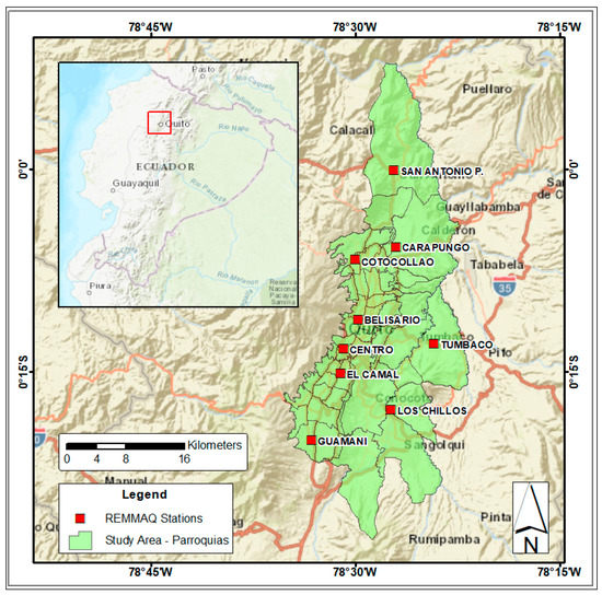
Figure 1.
Map of the study area (red dots for REEMAQ (Red Metropolitana de Monitoreo Atmosférico de Quito) stations and green polygons for urban parishes).
2.2. PM10 Data from AQMN Stations
In order to monitor air quality in Quito, nine stations have been acquiring air pollutants since 2002 (Figure 1). Together they form the “Red Metropolitana de Monitoreo Atmosférico de Quito” (REMMAQ) [37]. REEMAQ is the AQMN of Quito, where one of the air pollutants daily measured is PM10. These data are public and free to download (http://www.quitoambiente.gob.ec/ambiente/index.php/datos-horarios-historicos). The PM10 concentration is measured in micrograms per cubic meter (µg/m3). In this study, we use three-month-averages from 2013 to 2017, matching with the dates of the remote sensing data (time when the satellite passes over the study area). The main reasons to use three-month-averages are the few available remote sensing data and REMMAQ stations (stations without data in some months or with negative data values). In this study, PM10 three-month-averages are used as the dependent variable.
2.3. Remote Sensing Data Predictors
In this study, three different types of remote sensing data were used to retrieve PM10 between 2013 and 2017: Landsat-7 ETM+, Landsat-8 OLI/TIRS and MODIS/Terra and Aqua (Table 1). The remote sensing data are free to download from the United States Geological Survey (USGS) website (http://earthexplorer.usgs.gov). Moreover, only images with less than 10% cloud cover were considered in the study, because one of the main problems in these regions is the presence of a high cloud density [38,39]. According to this limitation, just 40% of remote sensing data was considered.

Table 1.
Characteristics of satellites and sensors used in the study.
The predictors or independent variables (surface reflectance bands and environmental indexes) are listed in Table 1. The selection of remote sensing predictors was related to their possible correlation with the PM10 concentration [9,40,41,42]. In the case of the environmental indexes, the most popular indexes in LUR studies to retrieve PM10 were used. They were computed as (1), (2), (3), (4), and (5) in Table 2, respectively.

Table 2.
Remote sensing predictors used to build the model for each sensor.
2.4. LUR Models
LUR models are an alternative to predict the spatialization of air pollutants, particularly when the number of AQMN stations is limited. They use different geographical variables such as roads, traffic information, meteorological and remote sensing data, and other environmental variables, in order to build a model to retrieve air pollutants. However, often several geographical variables are not available. Thus, we should use simple alternatives, such as free remote sensing data, as variables to approach a LUR model.
In most cases, LUR uses MLR to establish the model [47,48]. MLR allows an easy and simple model construction. In our case, the dependent variable is the quarterly PM10 value and the independent variables or spatial predictors are the remote sensing data in each coordinate of the AQMN station, considering the free cloud pixel value. Equation (6) shows the original LUR model, considering all the remote sensing predictors in MLR.
where I is the intercept, NDVI is normalized difference vegetation index, NDSI is the normalized difference soil index, SAVI is the soil-adjusted vegetation index, NDWI is the normalized difference water index, LST is the land surface temperature, B is the blue band, G is the green band, R is the red band, NIR is the near infrared band, SWIR is the shortwave infrared band, Y is the year of image acquisition, S is the three-month-averages of image acquisition (January–March—1, April–June—2, July–September—3, and October–November—4), a, b, …, l, are the coefficients in each predictor. The other variables are described in Table 1.
Nevertheless, considering that multicollinearity exists between remote sensing variables [31], different predictor techniques should be employed to compute the LUR model. We compare three techniques, namely, MLR with STW, PLS, and ANN, in order to find the fittest model (Figure 2).
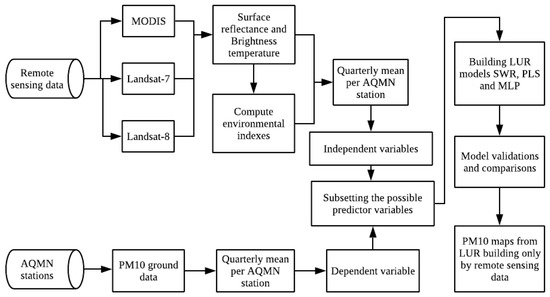
Figure 2.
Workflow of the methodology proposed to establish the land use regression (LUR) models.
In the first model, we use MLR considering an STW. It contemplates different parameters in order to identify the most adequate/influencing variables as predictors. The parameters used to subset the variables are: (i) The residual sum of squares for each model (RSS); (ii) the adjusted regression coefficient R2 (Adj. R2); (iii) Mallows’ Cp (CP) and; (iv) Bayesian information criterion (BIC).
The second model uses PLS with the STW criteria to select the predictors. The main challenge when using PLS is to avoid multicollinearity, finding an alternative when we have few data and a significant number of predictors [49]. PLS generates new latent variables or components in a lineal way.
Finally, the last model uses an ANN in an MLP, with a hidden layer and six hidden nodes to compute the predictive model. The nodes are computed according to [50]. In this model, we use all the predictors. This method is used when the model is complex, giving a different weight to each predictor corresponding to its importance. Additionally, we use a non-linear activation function with backpropagation. The training data to build the MLP consider 75% of the dataset and the remaining 25% for test. We use a backpropagation approach to train the algorithm. The R studio software was used in this study to extract the data and to compute all the models.
3. Results
PM10 ground measurements and remote sensing data are matched in a table with the same date. Thus, the unique condition is to consider remote sensing data with less than 10% cloud density. So, the three-month-averages matching tables for each sensor contain 35 observations for Landsat-7, 93 observations for Landsat-8, and 108 observations for MODIS. The main reasons to have only these numbers of observations are the high cloud density in the study area and the incomplete/not available air pollution data. Furthermore, the criteria to select predict variables consider five dependent variables for Landsat-7, eight dependent variables for Landast-8, and six dependent variables for MODIS, for each STW and PLS model, as shown in Table 3. They were obtained according to STW criteria (RSS, Adj. R2, CP, and BIC). The variables common to all the three cases considered are blue band, near infrared (NIR) band, and normalized difference vegetation index (NDVI).

Table 3.
Number of observations and predictors per satellite to build the LUR models.
The LUR models are computed considering STW and PLS regressions in a linear way and MLP in a non-linear way. They are shown and compared in Table 4 (Equations (7)–(12)). In the case of Landsat-7, the STW shows a coefficient of determination (R2) of 0.37, the PLS a R2 of 0.36, and, for MLP, a R2 of 0.46. The lowest root-mean-square error (RMSE) was obtained for STW with a value of 9.47. For Landsat-8, in STW a R2 of 0.42 was obtained, and a R2 of 0.43 for PLS, and a R2 of 0.68 for MLP (Figure 3). The lowest RMSE obtained was for MLP. Finally, for MODIS, a R2 of 0.15 for STW, a R2 of 0.19 for PLS and a R2 of 0.25 for MLP were obtained. The lowest RMSE was for STW.

Table 4.
LUR models for each sensor with different regression techniques. In the case of multilayer perceptron (MLP), the model is not linear.
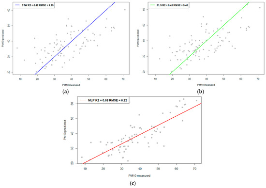
Figure 3.
Comparison between R2 and root mean square error (RMSE) in the model results for Landsat-8 data: (a) stepwise regression (STW); (b) partial least square (PLS); (c) MLP.
The results in Table 4 show that Landsat-8 data with MLP are the fittest model. The MLP employed (Figure 4) has one hidden layer with six hidden nodes.
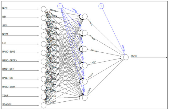
Figure 4.
MLP diagram for Landsat-8 data.
Figure 5 shows the relative variable importance according to the assigned weights, where the red band is the most significant in the model, while LST presented the lowest significance.
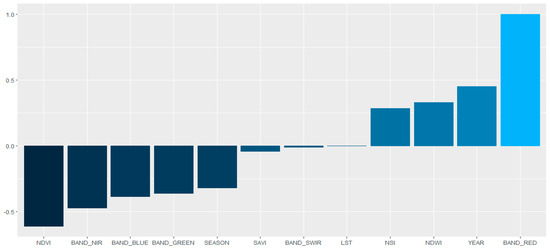
Figure 5.
Relative variable importance in Landsat-8 MLP. The scale is between −0.5 and 1, where 0 is the lowest (null) importance.
The Landsat-8 LUR-MLP model is chosen to predict PM10, considering the highest R2 and the lowest RMSE. In Figure 6, the quarterly maps show the PM10 spatial concentration during 2015, in a color scale in µg/m3. The white gaps showed in the maps are clouds with a high density.
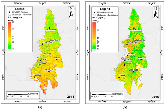
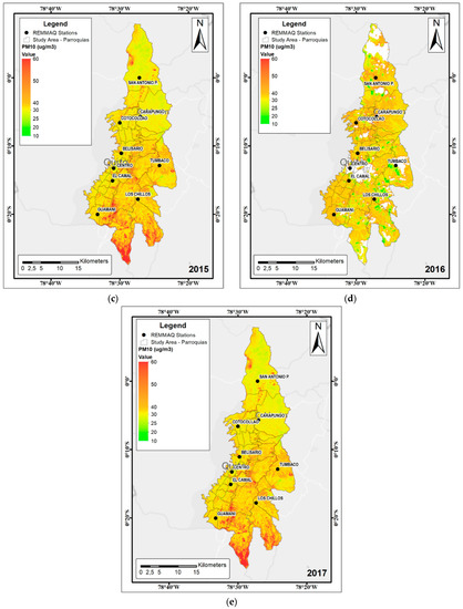
Figure 6.
PM10 concentrations during the season 4 (July to September) with Landsat-8 LUR-MLP model in: (a) 2013; (b) 2014; (c) 2015; (d) 2016; (e) 2017. The white gaps represent areas with a high cloud density.
4. Discussion
As demonstrated in this study, LUR models are an interesting alternative to model air quality, specifically PM10 concentrations, when the in-situ air quality measures are insufficient. Usually, most of the predictors are geographical variables (such as roads), traffic, meteorological data, and others [13]. LUR models are usually applied in small cities or regions where AQMN stations are limited [51], and where spatial interpolation techniques, such as ordinary kriging or inverse distance weighting, cannot be applied, considering the low number of ground measurements available [52]. One of the main problems with these geographic variables is the low accessibility to the data and the time of acquisition. Sometimes, these variables are obsolete, and they are not enough to establish a possible trend.
In this study, we propose an alternative, considering only free remote sensing variables. We apply this approach to the city of Quito, Ecuador, during the period between 2013 and 2017, in order to compare three different satellite data. Quito is growing in new poles. When REEMAQ was established in 2002, Quito did not have its current size and configuration. Now, REEMAQ is an obsolete air quality network, especially in the distribution of stations, which urgently needs improvement. Air pollutant spatial models are techniques based on interpolation or geostatistics approaches, which can be useful if a reasonable number of stations are available with a good spatial distribution [53]. In this study, only nine stations are available. Moreover, in some cases, the data are incomplete during some months. Additionally, according to some authors [7,8], it is possible to have more air ground data with low-cost sensors, however they must be implemented in the cities in order to monitor the air quality. The alternative to improve the air quality model in Quito is to establish different spatiotemporal LUR models, considering only remote sensing data as predictor variables. A preliminary study shows the use of only remote sensing variables but using an MLR in order to build the model. The limitation is the use of all remote sensing predictors without considering the collinearity [12]. In order to establish the models, three different remote sensing data were tested (Landsat-7, Landsat-8, and MODIS) and three techniques for modeling (STW, PLS, and MLP) were employed. The selected variables to compute the model are the visible NIR and SWIR bands of the three sensors, different environmental indices (NDVI, NDSI, SAVI, NDWI), and LST, computed from the data retrieved from each sensor. Most of the studies published use aerosol optical thickness (AOT) derived from MODIS (MOD04) [54] as the input in LUR models, however, this product has a low spatial resolution (3 × 3 km) [55]. This resolution is not practicable when considering cities like Quito, where the maximum width is near to 10 km. On the other hand, some MODIS products do not have a suitable quality for local studies [56]. Other studies use Landsat-8 combined with AOT ground stations to spatially model the AOT [24]. This could be a good alternative, however in our study area, we do not have access to this information between 2013 and 2017.
Comparing the LUR models established, we found that Landsat-8 is the most adequate sensor to model PM10 concentration, considering the 93 records and according to a previous study [12]. MLP is the fittest alternative to model PM10, with a R2 of 0.68 and a RMSE of 6.22. In this context, the non-linear model (MLP) has a fitter result when compared to the linear models (STW and PLS) [26]. Therefore, the LUR-MLP model was chosen to map the spatial concentration of PM10 in Quito, between 2013 to 2017. MODIS presents the lowest R2 with a value of 0.19, considering the PLS regression. This could be related to the lowest spatial resolution. Thus, most of the LUR models use MLR or STW. MLR is easy to implement. However, one of the main problems could be the multicollinearity, because MLR does not analyze the correlation between predictors [57]. On the other hand, the linear PLS helps to avoid the multicollinearity creating new latent variables with few observations [34]. In a future work, a possible combination between STW (in order to select the predictor variables), non-linear PLS (in order to avoid the multicollinearity between remote sensing data), and a machine learning technique (as ANN) can improve the LUR models [58].
In the case of the predictors, all the models present, in all the cases, the variables blue band, NIR, and NDVI. In the case of NDVI, a possible reason is the direct influence of vegetation on the PM10 concentration and distribution [18]. On the other hand, the red band has the most importance in MLP, because there could be a relationship between the retrieval of PM10 with the blue and red bands [27]. In most of the LUR studies, the authors use traffic, roads, meteorological, land use, population, and other predictors, reporting values of R2 according to the reality of each local [26]. These models also considered different time periods (monthly, quarterly, yearly). The main difference of our approach is the use of remote sensing data only as predictors, which can replace the necessity to have all geographical variables. Another advantage is the data availability and continuity in order to recompute the LUR models. One of the main limitations of our model is the high cloud density presented in the images during all the year [38], making it complicated to use more data in order to improve the model. However, a future work will intend to have more satellite sensors or to find new alternatives to recover remote sensing data contaminated with clouds [39].
Figure 6 shows variations year by year according to PM10 mean concentration based on in-situ data (REEMAQ Stations). We choose the third season to show the variation year by year (2013–2017), because we have more remote sensing data available (without a high cloud density) during this time-window. According to the results presented in Figure 6, an increasing of PM10 concentration between 2013 to 2017 is notorious in the most of the urban parishes [59]. However, some areas showed a decreasing tendency in some years. The lowest PM10 concentration was found in some peripheral parishes during the 2014 year, because the air stations that influence these parishes (Tumbaco and Los Chillos) had a variation in the concentrations. Thus, Tumbaco and Los Chillos stations are in the east part of the study area and began to present the lower values in 2014 followed by 2013, according to the in-situ measures. After 2014, the PM10 values for these stations began to increase. The main reason could be related to the new operation of the new airport of Quito (2013), and the construction of important road infrastructures around it (end of 2014). Another possible explication is the traffic influence during the last years, particularly in the peripheral areas where an increase was registered since 2015 and also the increase of the population in these areas [60]. In the northern parishes, the stations of San Antonio P. and Carapungo are influenced by the presence of stone and sandy point quarries [61]. The stations Centro, Belisario, and El Camal are in the city downtown, and it is the main reason that an increase of PM10 concentration during the last years is verified in the center parishes.
According to our results, several areas presented concentrations higher than 50 µg/m3 (Figure 6), while the World Health Organization (WHO) recommends, in its guidelines, maximum values of 20 µg/m3 as an annual mean and 50 µg/m3 as a 24-h mean [1]. However, some areas do not show values, due to the high cloud density (white areas in Figure 6). Thus, the PM10 concentration maps from the Landsat-8 LUR-MLP model can help local government decision makers to manage air quality concentration and to organize new policies, specifically in the places where the highest concentrations were identified.
5. Conclusions
In this study, three different satellite datasets were compared to retrieve models of PM10 through LUR, in Quito, Ecuador between 2013 and 2017. Additionally, three techniques were compared to compute the LUR models (SWR, PLS, and MLP). From this work, several conclusions could be taken: (i) It is possible to build empirical models established using only remote sensing variables as predictors without any other geographic variables, as traditional LUR models; (ii) in the case of Quito, the study results show that Landsat-8 provides the most suitable satellite data to retrieve PM10, in comparison with Landsat-7 and MODIS; (iii) MLP allows the obtainment of the most robust result in comparison with the other modeling techniques. MLP is the fittest alternative to model PM10, with a R2 of 0.68 and a RMSE of 6.22, and; (iv) the MLP model established helps in the spatial mapping of PM10, where in the time window of this study, were found areas with PM10 values higher than the limit established by WHO. Thus, these models are useful in the management of air quality in the city of Quito and can be applied to other locations with similar characteristics.
Author Contributions
Conceptualization, C.I.A.-M.; data curation, N.T. and V.V.; investigation, C.I.A.-M.; supervision, A.C.T.; writing—review and editing, C.I.A.-M.
Acknowledgments
The study is part of a PhD thesis in Surveying Engineering at the University of Porto, Portugal, supported by the Salesian Polytechnic University, Ecuador. This work was supervised at the University of Porto by Prof. Ana Cláudia Teodoro.
Conflicts of Interest
The authors declare no conflict of interest.
References
- WHO Ambient (Outdoor) Air Quality and Health. Available online: http://www.who.int/news-room/fact-sheets/detail/ambient-(outdoor)-air-quality-and-health (accessed on 30 August 2018).
- Kutlar Joss, M.; Eeftens, M.; Gintowt, E.; Kappeler, R.; Künzli, N. Time to harmonize national ambient air quality standards. Int. J. Public Health 2017, 62, 453–462. [Google Scholar] [CrossRef] [PubMed]
- Kobza, J.; Geremek, M.; Dul, L. Characteristics of air quality and sources affecting high levels of PM10 and PM2.5 in Poland, Upper Silesia urban area. Environ. Monit. Assess. 2018, 190, 515. [Google Scholar] [CrossRef] [PubMed]
- World Health Organization Regional Office for Europe. Health Effects of Particulate Matter; World Health Organization Regional Office for Europe: København, Denmark, 2013. [Google Scholar]
- Ielpo, P.; Paolillo, V.; de Gennaro, G.; Dambruoso, P.R. PM10 and gaseous pollutants trends from air quality monitoring networks in Bari province: Principal component analysis and absolute principal component scores on a two years and half data set. Chem. Cent. J. 2014, 8, 14. [Google Scholar] [CrossRef] [PubMed][Green Version]
- Pope, R.; Wu, J. A multi-objective assessment of an air quality monitoring network using environmental, economic, and social indicators and GIS-based models. J. Air Waste Manag. Assoc. 2014, 64, 721–737. [Google Scholar] [CrossRef] [PubMed]
- Capezzuto, L.; Abbamonte, L.; De Vito, S.; Massera, E.; Formisano, F.; Fattoruso, G.; Di Francia, G.; Buonanno, A. A maker friendly mobile and social sensing approach to urban air quality monitoring. In Proceedings of the IEEE SENSORS 2014, Valencia, Spain, 2–5 November 2014; pp. 12–16. [Google Scholar]
- Hasenfratz, D.; Saukh, O.; Walser, C.; Hueglin, C.; Fierz, M.; Thiele, L. Pushing the spatio-temporal resolution limit of urban air pollution maps. In Proceedings of the 2014 IEEE International Conference on Pervasive Computing and Communications (PerCom), Budapest, Hungary, 24–28 March 2014; pp. 69–77. [Google Scholar]
- Alvarez, C.I.; Padilla Almeida, O.; Álvarez Mendoza, C.I.; Padilla Almeida, O. Estimación de la contaminación del aire por PM10 en Quito a través de índices ambientales con imágenes LANDSAT ETM+. Rev. Cart 2016, 135–147. [Google Scholar]
- Cevallos, V.M.; Díaz, V.; Sirois, C.M. Particulate matter air pollution from the city of Quito, Ecuador, activates inflammatory signaling pathways in vitro. Innate Immun. 2017, 23, 392–400. [Google Scholar] [CrossRef] [PubMed]
- Raysoni, A.U.; Armijos, R.X.; Weigel, M.M.; Montoya, T.; Eschanique, P.; Racines, M.; Li, W.-W. Assessment of indoor and outdoor PM species at schools and residences in a high-altitude Ecuadorian urban center. Environ. Pollut. 2016, 214, 668–679. [Google Scholar] [CrossRef]
- Alvarez-Mendoza, C.I.; Teodoro, A.; Torres, N.; Vivanco, V.; Ramirez-Cando, L. Comparison of satellite remote sensing data in the retrieve of PM10 air pollutant over Quito, Ecuador. In Proceedings of the SPIE - The International Society for Optical Engineering, Berlin, Germany, 9 October 2018. [Google Scholar]
- Yang, X.; Zheng, Y.; Geng, G.; Liu, H.; Man, H.; Lv, Z.; He, K.; de Hoogh, K. Development of PM2.5 and NO2 models in a LUR framework incorporating satellite remote sensing and air quality model data in Pearl River Delta region, China. Environ. Pollut. 2017, 226, 143–153. [Google Scholar] [CrossRef]
- Stafoggia, M.; Schwartz, J.; Badaloni, C.; Bellander, T.; Alessandrini, E.; Cattani, G.; de’ Donato, F.; Gaeta, A.; Leone, G.; Lyapustin, A.; et al. Estimation of daily PM10 concentrations in Italy (2006–2012) using finely resolved satellite data, land use variables and meteorology. Environ. Int. 2017, 99, 234–244. [Google Scholar] [CrossRef]
- Shi, Y.; Lau, K.K.-L.; Ng, E. Incorporating wind availability into land use regression modelling of air quality in mountainous high-density urban environment. Environ. Res. 2017, 157, 17–29. [Google Scholar] [CrossRef]
- Son, Y.; Osornio-Vargas, Á.R.; O’Neill, M.S.; Hystad, P.; Texcalac-Sangrador, J.L.; Ohman-Strickland, P.; Meng, Q.; Schwander, S. Land use regression models to assess air pollution exposure in Mexico City using finer spatial and temporal input parameters. Sci. Total Environ. 2018, 639, 40–48. [Google Scholar] [CrossRef]
- Zou, B.; Chen, J.; Zhai, L.; Fang, X.; Zheng, Z.; Zou, B.; Chen, J.; Zhai, L.; Fang, X.; Zheng, Z. Satellite Based Mapping of Ground PM2.5 Concentration Using Generalized Additive Modeling. Remote Sens. 2016, 9, 1. [Google Scholar] [CrossRef]
- Wu, C.-D.; Chen, Y.-C.; Pan, W.-C.; Zeng, Y.-T.; Chen, M.-J.; Guo, Y.L.; Lung, S.-C.C. Land-use regression with long-term satellite-based greenness index and culture-specific sources to model PM2.5 spatial-temporal variability. Environ. Pollut. 2017, 224, 148–157. [Google Scholar] [CrossRef]
- He, J.; Zha, Y.; Zhang, J.; Gao, J. Aerosol indices derived from MODIS data for indicating aerosol-induced air pollution. Remote Sens. 2014, 6, 1587–1604. [Google Scholar] [CrossRef]
- Just, A.; De Carli, M.; Shtein, A.; Dorman, M.; Lyapustin, A.; Kloog, I.; Just, A.C.; De Carli, M.M.; Shtein, A.; Dorman, M.; et al. Correcting Measurement Error in Satellite Aerosol Optical Depth with Machine Learning for Modeling PM2.5 in the Northeastern USA. Remote Sens. 2018, 10, 803. [Google Scholar] [CrossRef]
- Wan, Z. MODIS Land Surface Temperature Products Users’ Guide; Institute for Computational Earth System Science, University of California: Santa Barbara, CA, USA, 2006. [Google Scholar]
- U.S. Geological Survey. Landsat—Earth Observation Satellites; Version 1.; U.S. Geological Survey: Reston, VA, USA, 2015; Volume 2015–3081.
- Olmanson, L.G.; Brezonik, P.L.; Finlay, J.C.; Bauer, M.E. Comparison of Landsat 8 and Landsat 7 for regional measurements of CDOM and water clarity in lakes. Remote Sens. Environ. 2016, 185, 119–128. [Google Scholar] [CrossRef]
- Bilal, M.; Nichol, J.E.; Bleiweiss, M.P.; Dubois, D. A Simplified high resolution MODIS aerosol retrieval algorithm (SARA) for use over mixed surfaces. Remote Sens. Environ. 2013, 136, 135–145. [Google Scholar] [CrossRef]
- Meng, X.; Fu, Q.; Ma, Z.; Chen, L.; Zou, B.; Zhang, Y.; Xue, W.; Wang, J.; Wang, D.; Kan, H.; et al. Estimating ground-level PM10 in a Chinese city by combining satellite data, meteorological information and a land use regression model. Environ. Pollut. 2016, 208, 177–184. [Google Scholar] [CrossRef]
- Shahraiyni, H.T.; Sodoudi, S. Statistical modeling approaches for pm10prediction in urban areas; A review of 21st-century studies. Atmosphere 2016, 7, 15. [Google Scholar] [CrossRef]
- Vermote, E.; Justice, C.; Claverie, M.; Franch, B. Preliminary analysis of the performance of the Landsat 8/OLI land surface reflectance product. Remote Sens. Environ. 2016, 185, 46–56. [Google Scholar] [CrossRef]
- Ayres-Sampaio, D.; Teodoro, A.C.; Sillero, N.; Santos, C.; Fonseca, J.; Freitas, A. An investigation of the environmental determinants of asthma hospitalizations: An applied spatial approach. Appl. Geogr. 2014, 47, 10–19. [Google Scholar] [CrossRef]
- Naughton, O.; Donnelly, A.; Nolan, P.; Pilla, F.; Misstear, B.D.; Broderick, B. A land use regression model for explaining spatial variation in air pollution levels using a wind sector based approach. Sci. Total Environ. 2018, 630, 1324–1334. [Google Scholar] [CrossRef]
- Li, X.; Zhang, Y.; Bao, Y.; Luo, J.; Jin, X.; Xu, X.; Song, X.; Yang, G. Exploring the Best Hyperspectral Features for LAI Estimation Using Partial Least Squares Regression. Remote Sens. 2014, 6, 6221–6241. [Google Scholar] [CrossRef]
- Chen, G.; Meentemeyer, R. Remote Sensing of Forest Damage by Diseases and Insects. In Remote Sensing for Sustainability; Weng, Q., Ed.; Remote Sensing Applications Series; CRC Press: Boca Raton, FL, USA, 2016; p. 357. ISBN 9781315354644. [Google Scholar]
- Xu, W.; Riley, E.A.; Austin, E.; Sasakura, M.; Schaal, L.; Gould, T.R.; Hartin, K.; Simpson, C.D.; Sampson, P.D.; Yost, M.G.; et al. Use of mobile and passive badge air monitoring data for NO X and ozone air pollution spatial exposure prediction models. J. Expo. Sci. Environ. Epidemiol. 2017, 27, 184–192. [Google Scholar] [CrossRef]
- Rosero-Vlasova, O.A.; Vlassova, L.; Pérez-Cabello, F.; Montorio, R.; Nadal-Romero, E. Modeling soil organic matter and texture from satellite data in areas affected by wildfires and cropland abandonment in Aragón, Northern Spain. J. Appl. Remote Sens. 2018, 12, 1. [Google Scholar] [CrossRef]
- Alvarez-Mendoza, C.I.; Teodoro, A.; Ramirez-Cando, L. Spatial estimation of surface ozone concentrations in Quito Ecuador with remote sensing data, air pollution measurements and meteorological variables. Environ. Monit. Assess. 2019, 191, 155. [Google Scholar] [CrossRef]
- Liu, W.; Li, X.; Chen, Z.; Zeng, G.; León, T.; Liang, J.; Huang, G.; Gao, Z.; Jiao, S.; He, X.; et al. Land use regression models coupled with meteorology to model spatial and temporal variability of NO2 and PM10 in Changsha, China. Atmos. Environ. 2015, 116, 272–280. [Google Scholar] [CrossRef]
- Gardner, M.; Dorling, S. Artificial neural networks (the multilayer perceptron)—A review of applications in the atmospheric sciences. Atmos. Environ. 1998, 32, 2627–2636. [Google Scholar] [CrossRef]
- Secretaria del Ambiente de Quito Red Metropolitana de Monitoreo Atmosférico de Quito. Available online: http://www.quitoambiente.gob.ec/ambiente/index.php/generalidades (accessed on 26 June 2018).
- Alvarez, C.I.; Teodoro, A.; Tierra, A. Evaluation of automatic cloud removal method for high elevation areas in Landsat 8 OLI images to improve environmental indexes computation. In Proceedings of the SPIE 10428, Earth Resources and Environmental Remote Sensing/GIS Applications VIII 1042809, Warsaw, Poland, 5 October 2017; Volume 10428, pp. 1042809–1042812. [Google Scholar]
- Alvarez-Mendoza, C.I.; Teodoro, A.; Ramirez-Cando, L. Improving NDVI by removing cirrus clouds with optical remote sensing data from Landsat-8—A case study in Quito, Ecuador. Remote Sens. Appl. Soc. Environ. 2019, 13, 257–274. [Google Scholar] [CrossRef]
- Othman, N.; Jafri, M.Z.M.; San, L.H. Estimating particulate matter concentration over arid region using satellite remote sensing: A case study in Makkah, Saudi Arabia. Mod. Appl. Sci. 2010, 4, 131. [Google Scholar] [CrossRef]
- Bilguunmaa, M.; Batbayar, J.; Tuya, S. Estimation of PM10 concentration using satellite data in Ulaanbaatar City. SPIE Asia Pac. Remote Sens. 2014, 92591O. [Google Scholar] [CrossRef]
- Ángel, M.; Gutiérrez, R. Uso de Modelos Lineales Generalizados (MLG) para la interpolación espacial de PM10 utilizando imágenes satelitales Landsat para la ciudad de Bogotá, Colombia. Perspectiva Geográfica. 2017, 22, 105–121. [Google Scholar] [CrossRef]
- Lee, J.H.; Ryu, J.E.; Chung, H.I.; Choi, Y.Y.; Jeon, S.W.; Kim, S.H. Development of spatial scaling technique of forest health sample point information. In Proceedings of the International Archives of the Photogrammetry, Remote Sensing and Spatial Information Sciences—ISPRS Archives, Beijing, China, 30 April 2018; Volume 42, pp. 751–756. [Google Scholar]
- Ghaleb, F.; Mario, M.; Sandra, A. Regional Landsat-Based Drought Monitoring from 1982 to 2014. Climate 2015, 3, 563–577. [Google Scholar] [CrossRef]
- Sobrino, J.A.; Jiménez-Muñoz, J.C.; Sòria, G.; Romaguera, M.; Guanter, L.; Moreno, J.; Plaza, A.; Martínez, P. Land surface emissivity retrieval from different VNIR and TIR sensors. IEEE Trans. Geosci. Remote Sens. 2008, 46, 316–327. [Google Scholar] [CrossRef]
- Li, S.; Jiang, G.M. Land Surface Temperature Retrieval from Landsat-8 Data with the Generalized Split-Window Algorithm. IEEE Access 2018, 6, 18149–18162. [Google Scholar] [CrossRef]
- Habermann, M.; Billger, M.; Haeger-Eugensson, M. Land use Regression as Method to Model Air Pollution. Previous Results for Gothenburg/Sweden. Procedia Eng. 2015, 115, 21–28. [Google Scholar] [CrossRef]
- Zhang, J.J.Y.; Sun, L.; Barrett, O.; Bertazzon, S.; Underwood, F.E.; Johnson, M. Development of land-use regression models for metals associated with airborne particulate matter in a North American city. Atmos. Environ. 2015, 106, 165–177. [Google Scholar] [CrossRef]
- Williams, L.J.; Abdi, H.; Williams, L.J. Partial Least Squares Methods: Partial Least Squares Correlation and Partial Least Square Regression. In Computational Toxicology: Volume II.; Reisfeld, B., Mayeno, A.N., Eds.; Humana Press: Totowa, NJ, USA, 2013; Volume 930, pp. 549–579. ISBN 978-1-62703-059-5. [Google Scholar]
- Sheela, K.G.; Deepa, S.N. Review on Methods to Fix Number of Hidden Neurons in Neural Networks. Math. Probl. Eng. 2013, 2013, 1–11. [Google Scholar] [CrossRef]
- Cattani, G.; Gaeta, A.; Di Menno di Bucchianico, A.; De Santis, A.; Gaddi, R.; Cusano, M.; Ancona, C.; Badaloni, C.; Forastiere, F.; Gariazzo, C.; et al. Development of land-use regression models for exposure assessment to ultrafine particles in Rome, Italy. Atmos. Environ. 2017, 156, 52–60. [Google Scholar] [CrossRef]
- Wang, M.; Sampson, P.D.; Hu, J.; Kleeman, M.; Keller, J.P.; Olives, C.; Szpiro, A.A.; Vedal, S.; Kaufman, J.D. Combining Land-Use Regression and Chemical Transport Modeling in a Spatiotemporal Geostatistical Model for Ozone and PM 2.5. Environ. Sci. Technol. 2016, 50, 5111–5118. [Google Scholar] [CrossRef]
- Alexeeff, S.E.; Schwartz, J.; Kloog, I.; Chudnovsky, A.; Koutrakis, P.; Coull, B.A. Consequences of kriging and land use regression for PM2.5 predictions in epidemiologic analyses: Insights into spatial variability using high-resolution satellite data. J. Expo. Sci. Environ. Epidemiol. 2015, 25, 138–144. [Google Scholar] [CrossRef]
- Beloconi, A.; Chrysoulakis, N.; Lyapustin, A.; Utzinger, J.; Vounatsou, P. Bayesian geostatistical modelling of PM10 and PM2.5 surface level concentrations in Europe using high-resolution satellite-derived products. Environ. Int. 2018, 121, 57–70. [Google Scholar] [CrossRef]
- Remer, L.A.; Mattoo, S.; Levy, R.C.; Munchak, L.A. MODIS 3 km aerosol product: Algorithm and global perspective. Atmos. Meas. Tech. 2013, 6, 1829–1844. [Google Scholar] [CrossRef]
- Teodoro, A. A study on the Quality of the Vegetation Index obtainded from MODIS Data. In Proceedings of the 2015 IEEE International Geoscience and Remote Sensing Symposium, Milan, Italy, 26–31 July 2015; pp. 3365–3368. [Google Scholar]
- Saucy, A.; Röösli, M.; Künzli, N.; Tsai, M.Y.; Sieber, C.; Olaniyan, T.; Baatjies, R.; Jeebhay, M.; Davey, M.; Flückiger, B.; et al. Land use regression modelling of outdoor NO2 and PM2.5 concentrations in three low income areas in the western cape province, South Africa. Int. J. Environ. Res. Public Health 2018, 15, 1452. [Google Scholar] [CrossRef]
- Lv, Y.; Liu, J.; Yang, T. Nonlinear PLS Integrated with Error-Based LSSVM and Its Application to NO2 Modeling. Ind. Eng. Chem. Res. 2012, 51, 16092–16100. [Google Scholar] [CrossRef]
- Secretaria del Ambiente de Quito. IAMQ/18; Secretaria del Ambiente de Quito: Quito, Ecuador, 2018.
- Romero, D.; El parque automotor aumenta y complica más la movilidad. El Comer. 2017, 1. Available online: https://www.elcomercio.com/actualidad/aumento-parque-automotor-quito-movilidad.html (accessed on 13 June 2019).
- Todoroski Air Sciences. Air Quality Impact Assessment Sandy Point Quarry Epl Variation; Todoroski Air Sciences: Eastwood, Australia, 2019. [Google Scholar]
© 2019 by the authors. Licensee MDPI, Basel, Switzerland. This article is an open access article distributed under the terms and conditions of the Creative Commons Attribution (CC BY) license (http://creativecommons.org/licenses/by/4.0/).