An Open Source GIS-Based Application for the Assessment of Groundwater Vulnerability to Pollution


Abstract
1. Introduction
2. Materials and Methods
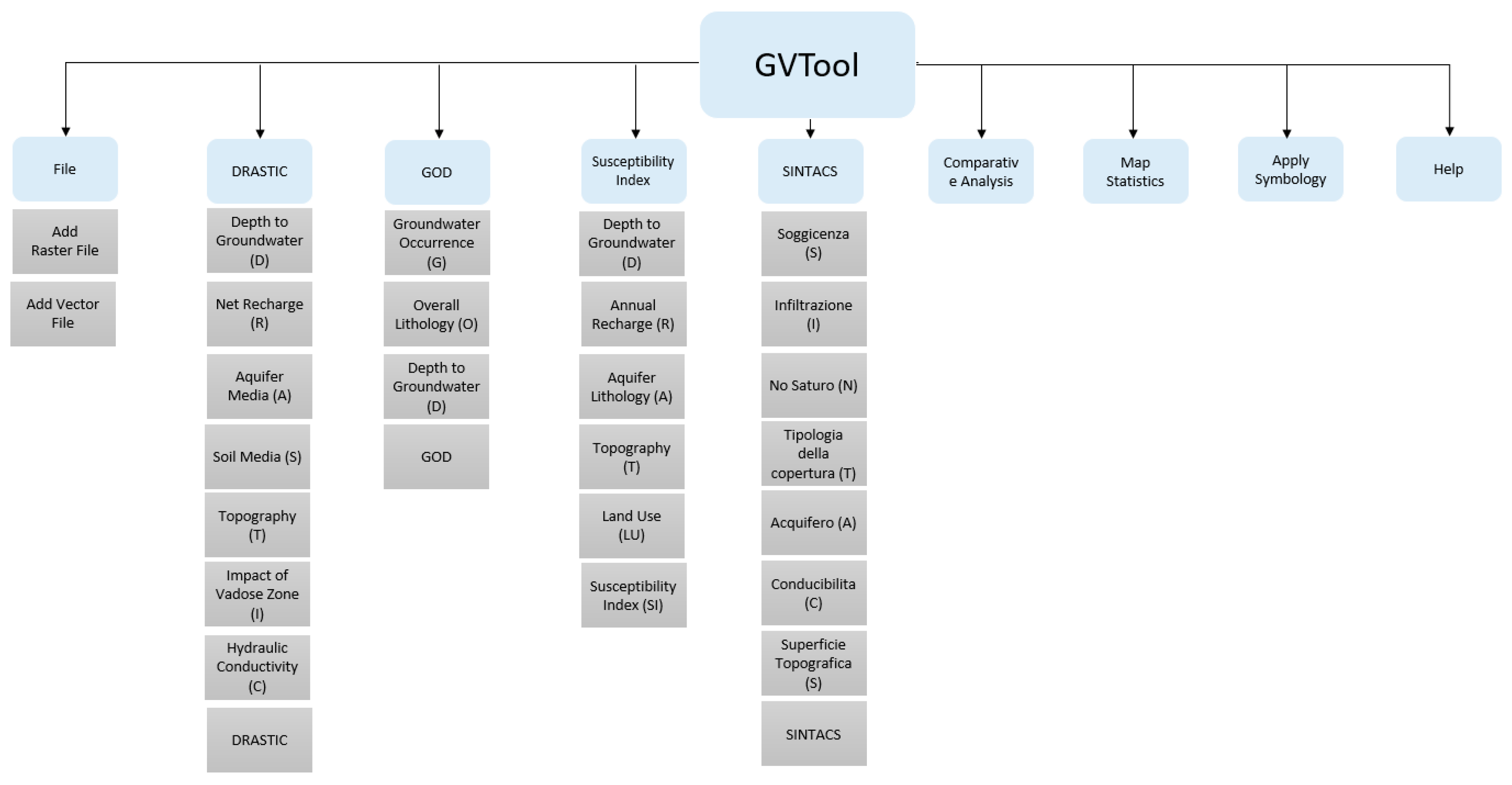
2.1. QGIS Open Source Software
- besides the DRASTIC vulnerability index, the application includes GOD, SINTACS, and SI methods;
- a Comparative Analysis menu, which provides the users several alternatives to compare groundwater vulnerability maps obtained by applying different methods to the same area;
- a Map Statistics menu capable of performing statistical analysis of a raster;
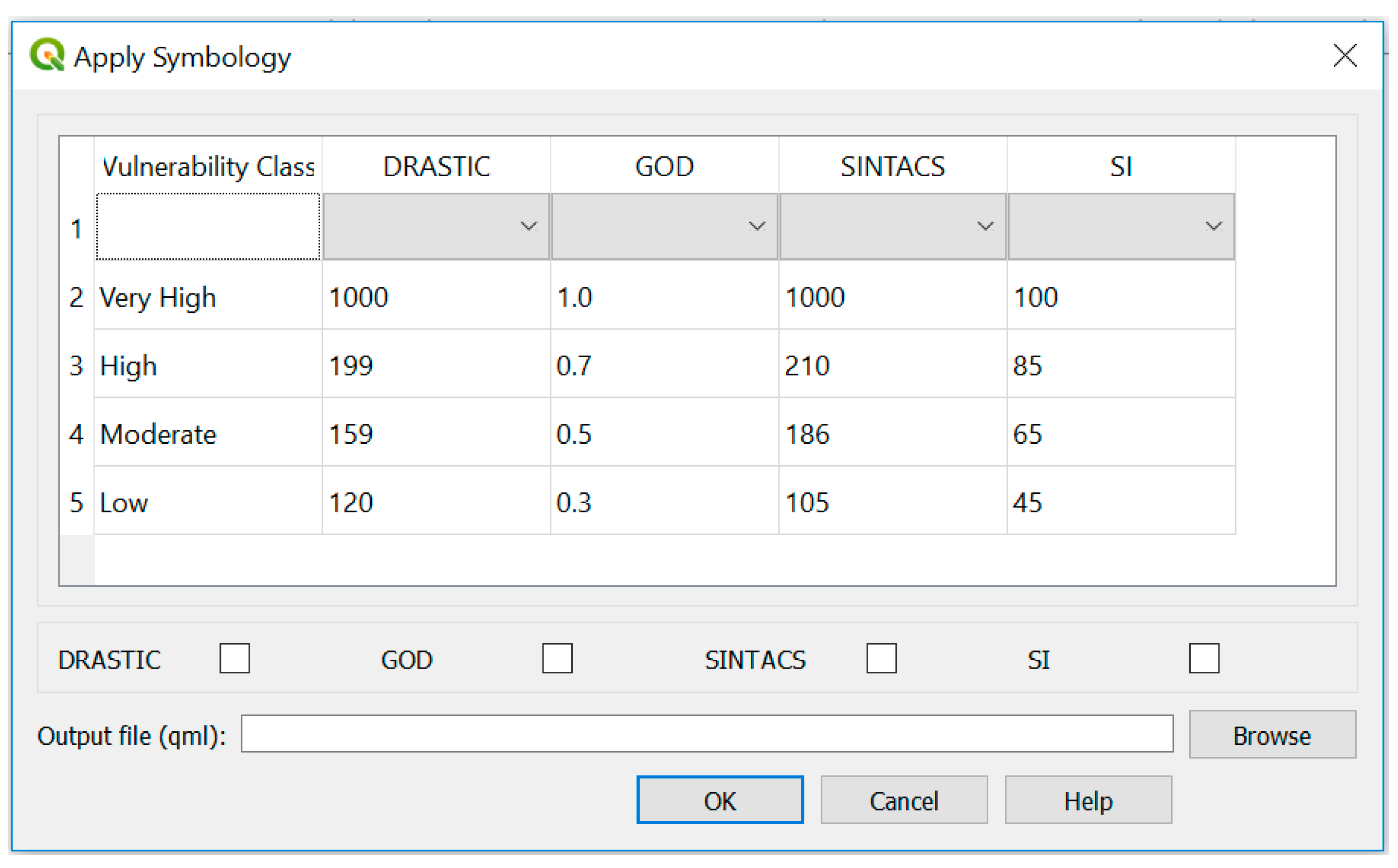
- a Symbology menu was created to provide the user the capability of redefining vulnerability classes and to apply the respective symbology to a map or a set of maps.
2.2. Implemented Groundwater Vulnerability Assessment Methods
2.2.1. DRASTIC
2.2.2. GOD
- the type of groundwater confinement (G factor), varying from 0 (corresponding to none or overflowing) to 1.0 (corresponding to unconfined);
- the characteristics of the overlying strata (O factor), namely, the lithological character and degree of consolidation of the vadose zone or the confining beds (ranging from 0.4 in the case of lacustrine/estuarine clays to 1.0 in the case of karst limestones);
- the D factor encompasses depth to groundwater table (for unconfined aquifers) or to groundwater strike (for confined aquifers), ranging from 0.6 (depth greater than 50 m) to 1.0 (for all depths in the case of karstic aquifers). The GOD index is calculated through the multiplication of these three factors (Equation (2)):GOD = G × O × D
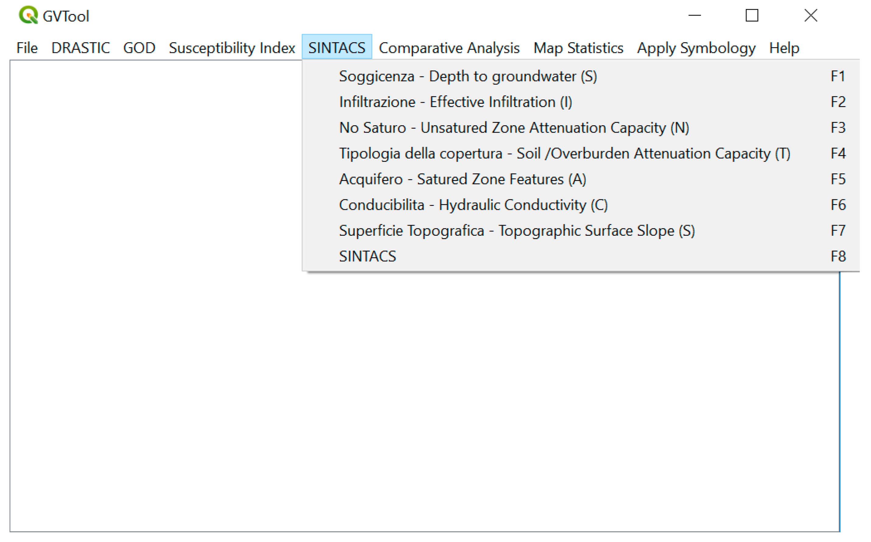
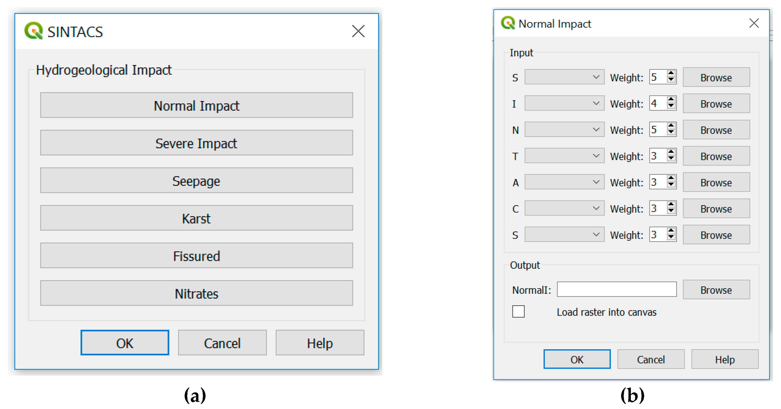
2.2.3. SINTACS
2.2.4. Susceptibility Index (SI)
3. Implementation of GVTool
3.1. Depth to Groundwater
3.2. Net Recharge
3.3. Factors Related to Soil, to The Unsaturated Zone, and to Aquifer Features
3.4. Topography
3.5. Hydraulic Conductivity
3.6. SINTACS Soggicenza, Infiltrazione, Conducibilita, and Superficie Topografica Factors
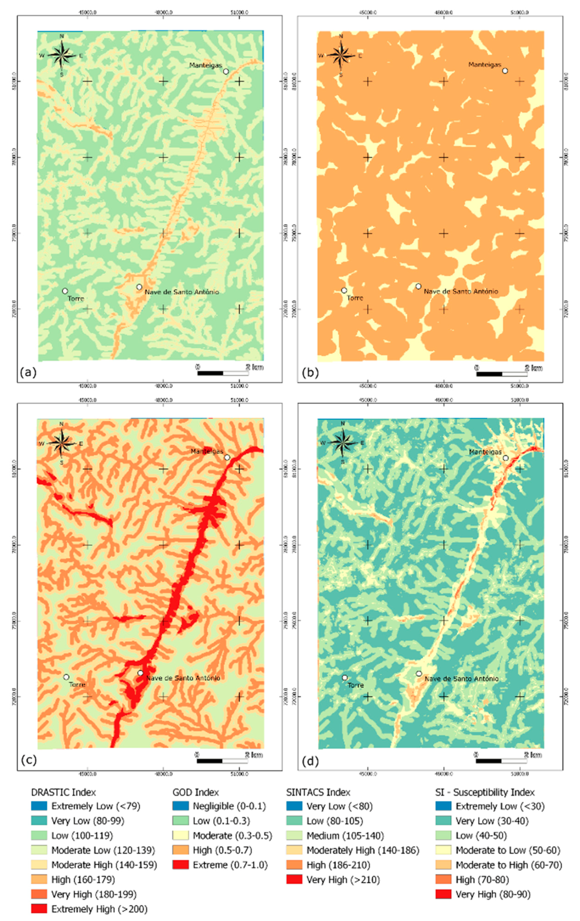
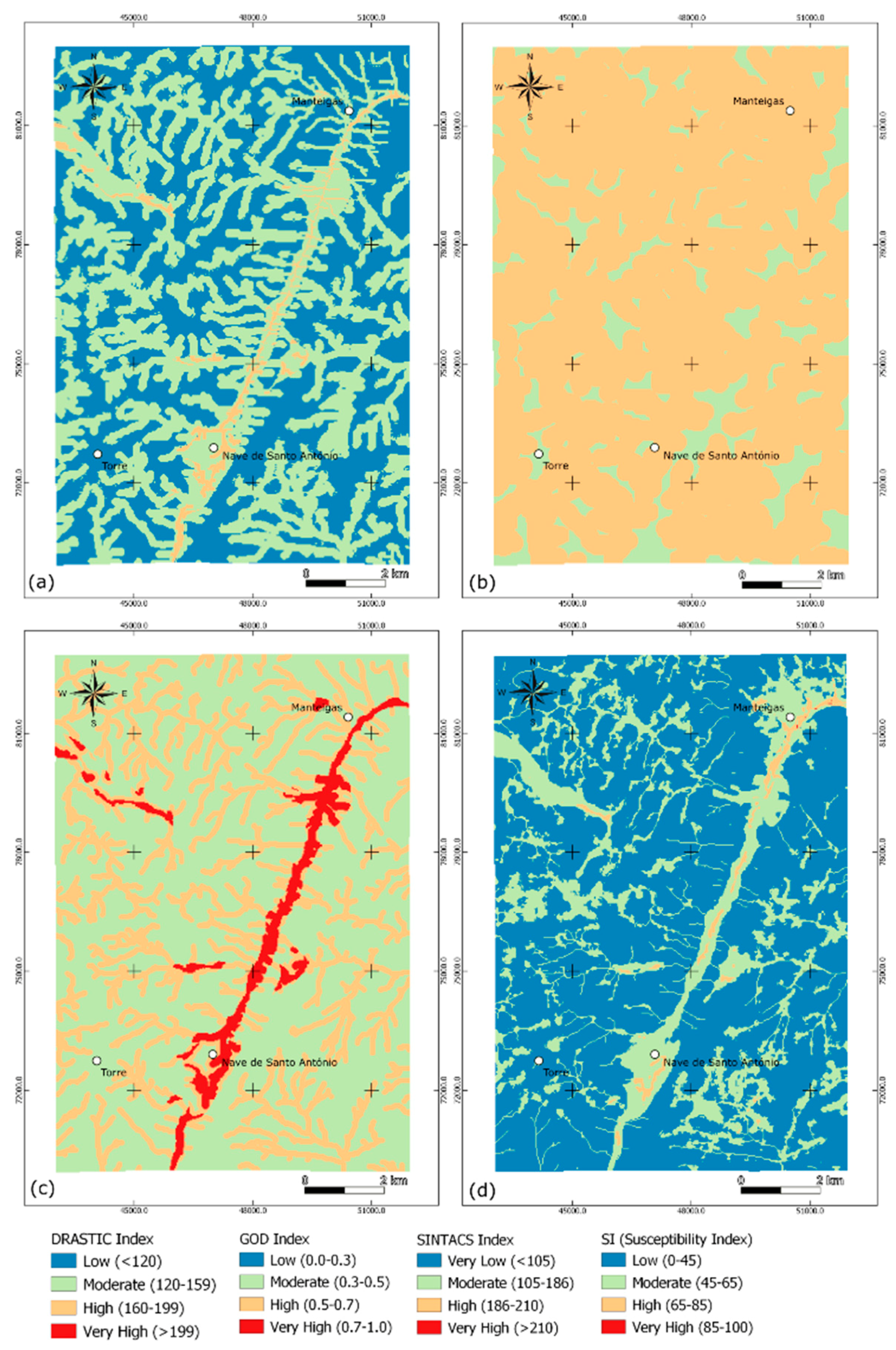
3.7. Final Maps
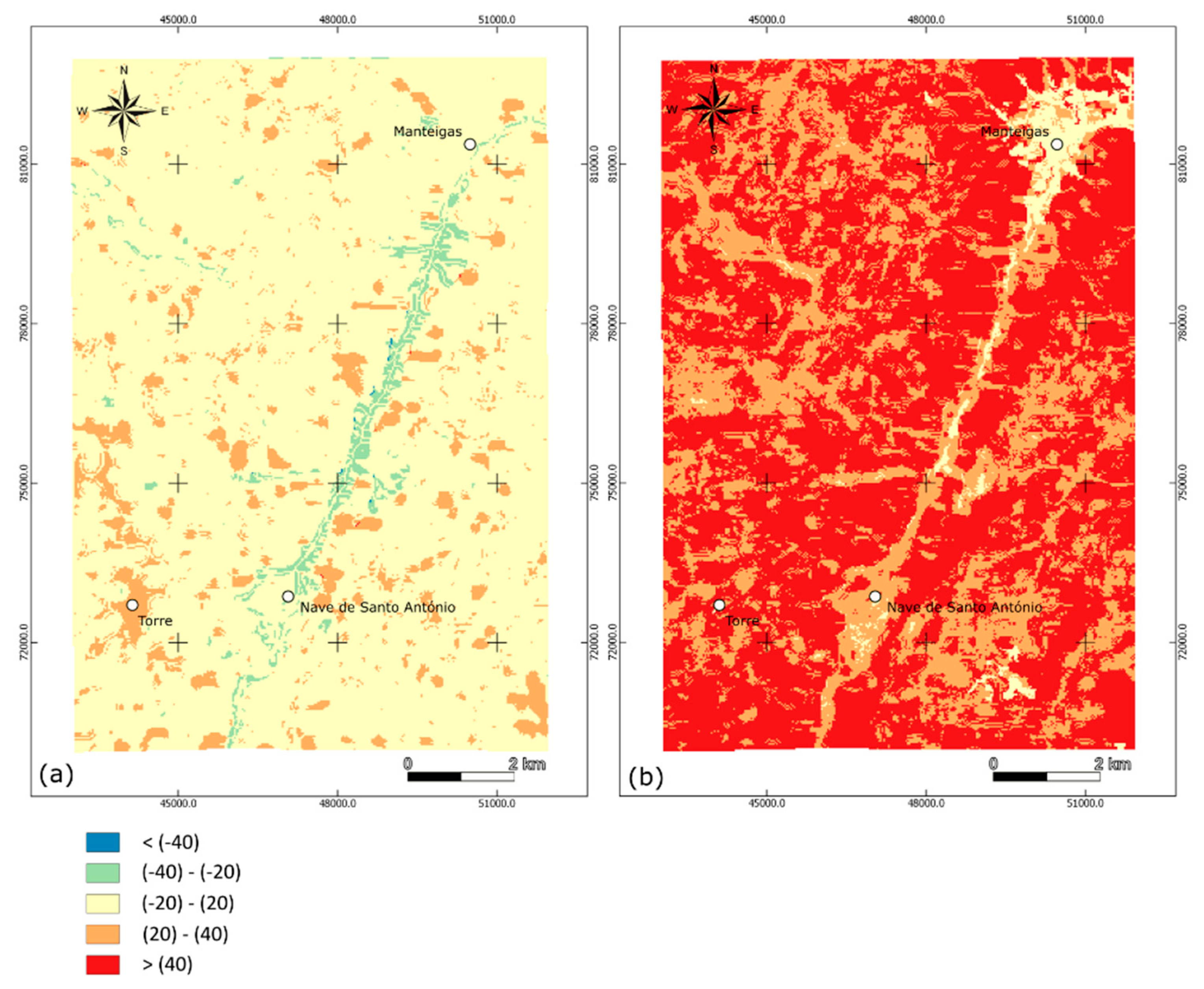
3.8. Comparative Analysis Menu Implementation
3.9. Map Statistics
3.10. Apply Symbology
4. GVTool Illustrative Application
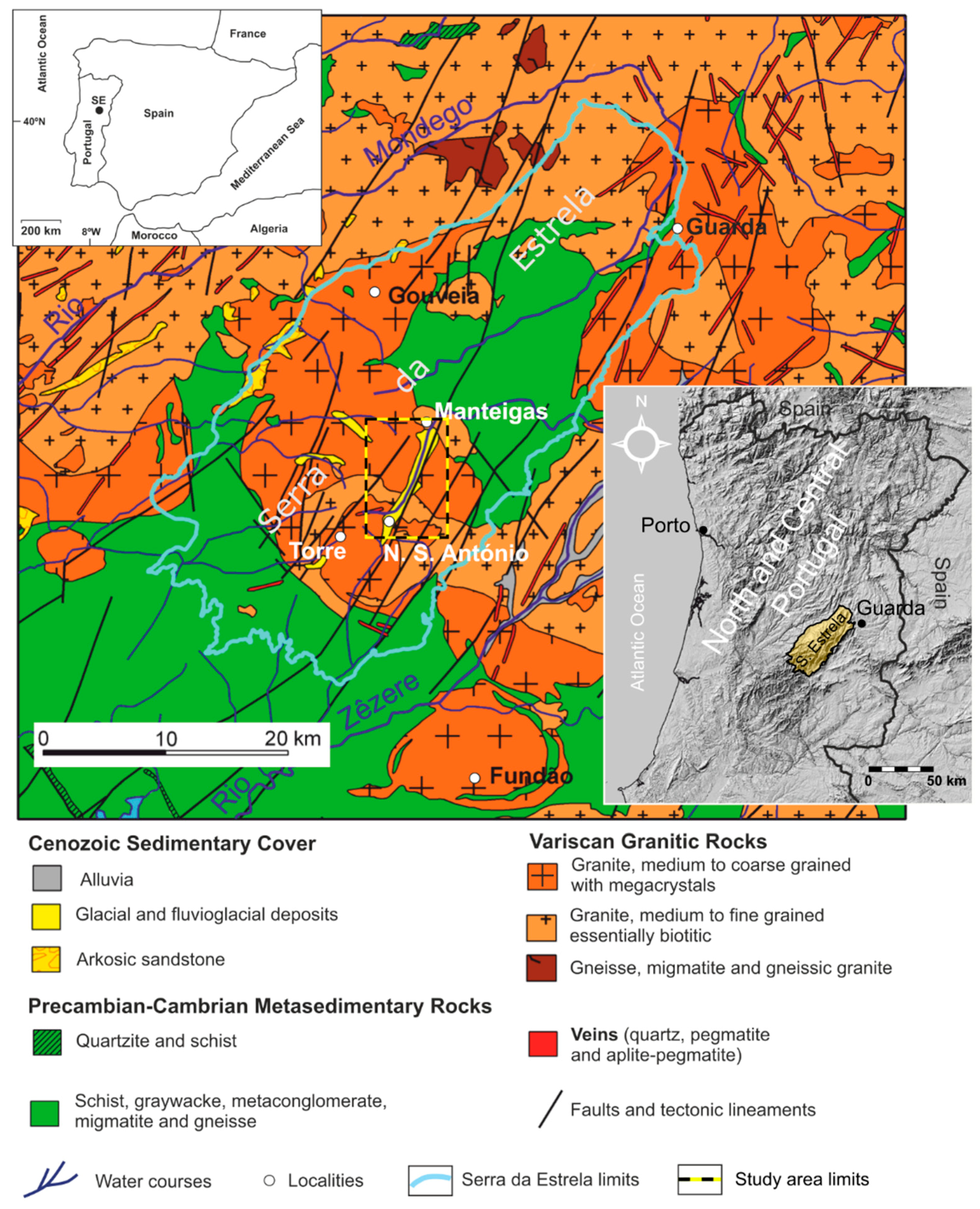
4.1. Hydrogeological Framework
4.2. Application of GVTool to The Region of Serra da Estrela
5. Conclusions
Author Contributions
Acknowledgments
Conflicts of Interest
References
- Ross, A. Groundwater Governance in Australia, the European Union and the Western USA. In Integrated Groundwater Management: Concepts, Approaches and Challenges; Jakeman, A.J., Barreteau, O., Hunt, R.J., Rinaudo, J., Ross, A., Eds.; Springer: Cham, Switzerland, 2016. [Google Scholar] [CrossRef]
- Margat, J.; van der Gun, J. Groundwater around the World, A Geographic Synopsis; CRC Press: Boca Raton, FL, USA, 2013; ISBN 978-0-203-77214-0. [Google Scholar]
- Nwankwoala, H.O. Groundwater and Poverty Reduction: Challenges and Opportunities for Sustainable Development in Nigeria. Hydrol. Curr. Res. 2016, 7, 2. [Google Scholar] [CrossRef]
- EC. Directive 2000/60/EC of the European Parliament and of the Council Establishing a Framework for Community Action in the Field of Water Policy; OJ L 327, 22 December 2000; Office for Official Publications of the European Communities: Luxembourg, 2000. [Google Scholar]
- EC. Directive 2006/118/EC of the European Parliament and of the Council on the Protection of Groundwater Against Pollution and Deterioration; OJ L 372, 27 December 2006; Office for Official Publications of the European Communities: Luxembourg, 2006. [Google Scholar]
- Navarrete, C.M.; Olmedo, J.G.; Valsero, J.J.D.; Gómez, J.D.G.; Espinar, J.A.L.; Gómez, J.A.O. Groundwater protection in Mediterranean countries after the European water framework directive. Environ. Geol. 2008, 54, 537–549. [Google Scholar] [CrossRef]
- Hérivaux, C.; Grémont, M. Valuing a diversity of ecosystem services: The way forward to protect strategic groundwater resources for the future? Ecosyst. Serv. 2019, 35, 184–193. [Google Scholar] [CrossRef]
- Wachniew, P.; Zurek, A.J.; Stumpp, C.; Gemitzi, A.; Gargini, A.; Filippini, M.; Rozanski, K.; Meeks, J.; Kværner, J.; Witczak, S. Toward operational methods for the assessment of intrinsic groundwater vulnerability: A review. Crit. Rev. Environ. Sci. Technol. 2016, 46, 827–884. [Google Scholar] [CrossRef]
- Shende, S.; Chau, K. Forecasting Safe Distance of a Pumping Well for Effective Riverbank Filtration. J. Hazard. Toxic Radioact. Waste 2019, 23. [Google Scholar] [CrossRef]
- Van Duijvenbooden, W.V.; Waegeningh, H.G. Vulnerability of Soil and Groundwater to Pollutants. In Proceedings and Information No. 38 of International Conference Held in the Netherlands; TNO Committee on Hydrological Research: Delft, The Netherlands, 1987. [Google Scholar]
- Krogulec, E. Intrinsic and Specific Vulnerability of Groundwater in a River Valley—Assessment, Verification and Analysis of Uncertainty. Earth Sci. Clim. Chang. 2013, 4. [Google Scholar] [CrossRef]
- Vrba, J.; Zaporozec, A. Guidebook on Mapping Groundwater Vulnerability, IAH, International Contributions to Hydrogeology, 16; Heise: Hannover, Germany, 1994. [Google Scholar]
- Lai, Y.; Wang, F.; Zhang, Y.; Li, S.; Wu, P.; Ou, P.; Fang, Q.; Chen, Z.; Duan, Y. Implementing chemical mass balance model and vulnerability the theories to realize the comprehensive evaluation in an abandoned battery plant. Sci. Total Environ. 2019, 686, 788–796. [Google Scholar] [CrossRef]
- Kong, M.; Zhong, H.; Wu, Y.; Liu, G.; Xu, Y.; Wang, G. Developing and validating intrinsic groundwater vulnerability maps in regions with limited data: A case study from Datong City in China using DRASTIC and Nemerow pollution indices. Environ. Earth Sci. 2019, 78, 262. [Google Scholar] [CrossRef]
- Machiwal, D.; Jha, M.K.; Singh, V.P.; Mohan, C. Assessment and mapping of groundwater vulnerability to pollution: Current status and challenges. Earth-Sci. Rev. 2018, 185, 901–927. [Google Scholar] [CrossRef]
- Aller, L.; Bennett, T.; Lehr, J.H.; Petty, R.J.; Hackett, G. DRASTIC: A Standardized System for Evaluating Ground Water Pollution Potential Using Hydrogeologic Settings; EPA-600/2-87-035; EPA: Washington, DC, USA, 1987.
- Foster, S.; Hirata, R.; Gomes, D.; Delia, M.; Paris, M. Groundwater Quality Protection: A Guide for Water Utilities, Municipal Authorities, and Environment Agencies; The International Bank for Reconstruction and Development; The World Bank: Washington, DC, USA, 2002. [Google Scholar]
- Moore, P.; John, S. SEEPAGE: A System for Early Evaluation of the Pollution Potential of Agricultural Groundwater Environments; Geology Technical Note; USDA, SCS, Northeast Technical Center: Chester, PA, USA, 1990.
- Van Stempvoort, D.; Ewert, L.; Wassenaar, L. Aquifer vulnerability index: A GIS-compatible method for groundwater vulnerability mapping. Can. Water Resour. J. 2013, 18, 25–37. [Google Scholar] [CrossRef]
- Civita, M. Le Carte Della Vulnerabilita Degli acquiferiall’inquinamento Teoria and Practica (Aquifer Vulnerability Maps to Pollution); Pitagora Editrice: Bologna, Italy, 1994. [Google Scholar]
- Civita, M.; De Maio, M. SINTACS Un Sistema Parametrico per la Valutazione e la Cartografia per la Valutazione Della Vulnerabilita`Degli Acquiferi All’inquinamento, Metodologia e Automazione; Pitagora Editrice: Bologna, Italy, 1997. [Google Scholar]
- Doerfliger, N.; Zwahlen, F. EPIK: A new method for outlining of protection areas in karst environment. In Proceedings of the 5th International Symposium and Field Seminar on Karst Waters and Environmental Impacts, Antalya, Turkey, 10–20 September 1995; Gunay, G., Johnson, I., Eds.; Balkema: Rotterdam, The Netherlands, 1995; pp. 117–123. [Google Scholar]
- Civita, M.; De Regibus, C. Sperimentazione di alcune metodologie per la valutazione della vulnerabilita degli aquifer. Quad. Geol. Appl. 1995, 3, 63–72. [Google Scholar]
- Davis, A.D.; Long, A.J.; Wireman, M. KARSTIC: A sensitivity method for carbonate aquifers in karst terrain. Environ. Geol. 2002, 42, 65–72. [Google Scholar] [CrossRef]
- Stigter, T.Y.; Ribeiro, L.; Dill, A.M. Evaluation of an intrinsic and a specific vulnerability assessment method in comparison with groundwater salinisation and nitrate contamination levels in two agricultural regions in the south of Portugal. Hydrogeol. J. 2006, 14, 79–99. [Google Scholar] [CrossRef]
- Jarray, H.; Zammouri, M.; Ouessar, M.; Zerrim, A.; Yahyaoui, H. GIS based DRASTIC Model for Groundwater Vulnerability Assessment: Case Study of the Shallow Mio-Plio Quaternary Aquifer (Southeastern Tunisia). Water Resour. 2017, 44, 595–603. [Google Scholar] [CrossRef]
- Edet, A. An aquifer vulnerability assessment of the Benin Formation aquifer, Calabar, southeastern Nigeria, using DRASTIC and GIS approach. Environ. Earth Sci. 2014, 71, 1747–1765. [Google Scholar] [CrossRef]
- Asadi, P.; Ataie-Ashtiani, B.; Beheshti, A. Vulnerability assessment of urban groundwater resources to nitrate: The case study of Mashhad, Iran. Environ. Earth Sci. 2017, 76, 41. [Google Scholar] [CrossRef]
- Meerkhan, H.; Teixeira, J.; Espinha Marques, J.; Afonso, M.J.; Chaminé, H.I. Delineating Groundwater Vulnerability and Protection Zone Mapping in Fractured Rock Masses: Focus on the DISCO Index. Water 2016, 8, 462. [Google Scholar] [CrossRef]
- Draoui, M.; Vias, J.; Andreo, B.; Targuisti, K.; Stitou El Messari, J. A comparative study of four vulnerability mapping methods in a detritic aquifer under mediterranean climatic conditions. Environ. Geol. 2007, 54, 455–463. [Google Scholar] [CrossRef]
- Aschonitis, V.G.; Castaldelli, G.; Colombani, N.; Mastrocicco, M. A combined methodology to assess the intrinsic vulnerability of aquifers to pollution from agrochemicals. Arab. J. Geosci. 2016, 9, 503. [Google Scholar] [CrossRef]
- Oroji, B. Groundwater vulnerability assessment using GIS-based DRASTIC and GOD in the Asadabad plain. J. Mater. Environ. Sci. 2018, 9, 1809–1816. [Google Scholar]
- Yousefi, H.; Haghizadeh, A.; Yarahmadi, Y.; Hasanpour, P.; Noormohamadi, P. Groundwater pollution potential evaluation in Khorramabad-Lorestan Plain, western Iran. J. Afr. Earth Sci. 2018, 147, 647–656. [Google Scholar] [CrossRef]
- Yildirim, M.; Topkaya, B. Groundwater Protection: A Comparative Study of Four Vulnerability Mapping Methods. Clean 2007, 35, 594–600. [Google Scholar]
- Saida, S.; Tarik, H.; Abdellah, A.; Farid, H.; Hakiml, B. Assessment of Groundwater Vulnerability to Nitrate Based on the Optimised DRASTIC Models in the GIS Environment (Case of Sidi Rached Basin, Algeria). Geosciences 2017, 7, 20. [Google Scholar] [CrossRef]
- Pisciotta, A.; Cusimano, G.; Favara, R. Groundwater nitrate risk assessment using intrinsic vulnerability methods: A comparative study of environmental impact by intensive farming in the Mediterranean region of Sicily, Italy. J. Geochem. Explor. 2015, 156, 89–100. [Google Scholar] [CrossRef]
- Stallman, P. Why ‘Open Source’ Misses the Point of Free Software, GNU Operating System. Available online: http://www.gnu.org/philosophy/open-sourcemisses-the-point.html (accessed on 10 February 2019).
- QGIS Project. Available online: http://www.qgis.org/ (accessed on 10 November 2018).
- Groundwater Vulnerability Mapping Plugin, Hosted in QGIS Official Repository (from Christian Boehnke). Available online: https://plugins.qgis.org/plugins/GroundwaterVulnerability/ (accessed on 10 June 2019).
- Ollivier, C.; Lecomte, Y.; Chalikakis, K.; Mazzilli, N.; Danquigny, C.; Emblanch, C. A QGIS Plugin Based on the PaPRIKa Method for Karst Aquifer Vulnerability Mapping. Groundwater 2019, 57, 201–204. [Google Scholar] [CrossRef]
- Rossetto, R.; De Filippis, G.; Borsi, I.; Foglia, L.; Cannata, M.; Criollo, R.; Vázquez-Suñé, E. Integrating free and open source tools and distributed modelling codes in GIS environment for data-based groundwater management. Environ. Model. Softw. 2018, 107, 210–230. [Google Scholar] [CrossRef]
- Duarte, L.; Teodoro, A.C.; Gonçalves, J.A.; Guerner Dias, A.J.; Espinha Marques, J. A dynamic map application for the assessment of groundwater vulnerability to pollution. Environ. Earth Sci. 2015, 74, 2315–2327. [Google Scholar] [CrossRef]
- Processing Toolbox. Available online: https://github.com/qgis/QGIS/wiki/Plugin-migration-to-QGIS-3 (accessed on 10 March 2019).
- Afonso, M.J.; Freitas, L.; Pereira, A.J.S.C.; Neves, L.J.P.F.; Guimarães, L.; Guilhermino, L.; Mayer, B.; Rocha, F.; Marques, J.M.; Chaminé, H.I. Environmental Groundwater Vulnerability Assessment in Urban Water Mines (Porto, NW Portugal). Water 2016, 8, 499. [Google Scholar] [CrossRef]
- Ouedraogo, I.; Defourny, P.; Vanclooster, M. Mapping the groundwater vulnerability for pollution at the pan African scale. Sci. Total Environ. 2016, 544, 939–953. [Google Scholar] [CrossRef]
- Foster, S.S.D. Fundamental concepts in aquifer vulnerability, pollution risk and protection strategy. In Vulnerability of Soil and Groundwater to Pollution; Proceedings and Information No. 38 of the International Conference held in the Netherlands, in 1987; van Duijvanbooden, W., van Waegeningh, H.G., Eds.; TNO Committee on Hydrological Research: Delft, The Netherlands, 1987. [Google Scholar]
- Al Kuisi, M.; El-Naqa, A.; Hammouri, N. Vulnerability mapping of shallow groundwater aquifer using SINTACS model in the Jordan Valley area, Jordan. Environ. Geol. 2006, 50, 651. [Google Scholar] [CrossRef]
- Francés, A.; Paralta, E.; Fernandes, J.; Ribeiro, L. Development and application in the Alentejo region of a method to assess the vulnerability of groundwater to diffuse agriculture pollution: The susceptibility index. In Proceedings of the Third International Conference on Future Groundwater Resources at Risk, Lisbon, Portugal, 25–27 June 2001; GeoSystem Center IST: Lisboa, Portugal, 2001. [Google Scholar]
- DGT (Direção Geral do Território). Available online: http://www.dgterritorio.pt/dados_abertos/clc/ (accessed on 13 March 2019).
- Bonham-Carter, G.F. Geographic Information Systems for Geoscientists, Modelling with GIS. Comput. Method Geosci. 1994, 13, 152–153. [Google Scholar]
- Deutsch, C.; Journel, A. GSLIB: Geostatistical Software Library and User’s Guide; Oxford University Press: Oxford, UK, 1992; p. 340. [Google Scholar]
- Haber, J.; Zeilfelder, F.; Davydov, O.; Seidel, H.P. Smooth approximation and rendering of large scattered data sets. In Proceedings of the IEEE Visualization, San Diego, CA, USA, 21–26 October 2001; Joy, T.E.K., Varshney, A., Eds.; IEEE Computer Society: Washington, DC, USA, 2001; Volume 571, pp. 341–347. [Google Scholar]
- Mitasova, H.; Mitas, L.; Brown, B.M.; Gerdes, D.P.; Kosinovsky, I. Modeling spatially and temporally distributed phenomena: New methods and tools for GRASS GIS. Int. J. GIS Spec. Issue Integr. GIS Environ. Model 1995, 9, 433–446. [Google Scholar]
- Mitasova, H.; Mitas, L.; Harmon, R.S. Simultaneous spline approximation and topographic analysis for lidar elevation data in open source GIS. IEEE GRSL 2005, 2, 375–379. [Google Scholar] [CrossRef]
- Jansen, J.; Sequeira, M.P.S.M. The vegetation of shallow waters and seasonally inundated habitats (Littorelletea and Isoeto-Nanojuncetea) in the higher parts of the Serra da Estrela, Portugal. Mitt. Badischen Landesver. Naturkunde 1999, 17, 449–462. [Google Scholar]
- Mora, C. A synthetic map of the climatopes of the Serra da Estrela (Portugal). J. Maps 2010, 6, 591–608. [Google Scholar] [CrossRef]
- AEMET-IM. Iberian Climate Atlas, Air Temperature and Precipitation (1971–2000); Ministerio de Medio Ambiente, Medio Rural y Marino: Madrid, Spain, 2011. [Google Scholar]
- Daveau, S.; Coelho, C.; Costa, V.G.; Carvalho, L. Distribution and Rhythm of Precipitation in Portugal; Memórias do Centro de Estudos Geográficos: Lisbon, Portugal, 1977. (In French) [Google Scholar]
- Vieira, G.T.; Mora, C. General characteristics of the climate of the Serra da Estrela. In Glaciar Periglacial Geomorphology of the Serra da Estrela, Guidebook for the Field-Trip; IGU Commission on Climate Change and Periglacial Environments, 26–28 August 1998; Vieira, G.T., Ed.; CEG and Department of Geology, University of Lisbon: Lisbon, Portugal, 1998; pp. 26–36. [Google Scholar]
- Espinha Marques, J.; Duarte, J.M.; Constantino, A.T.; Martins, A.A.; Aguiar, C.; Rocha, F.T.; Inácio, M.; Marques, J.M.; Chaminé, H.I.; Teixeira, J.; et al. Vadose zone characterisation of a hydrogeologic system in a mountain region: Serra da Estrela case study (Central Portugal). In Aquifer Systems Management: Darcy’s Legacy in a World of Impending Water Shortage; SP-10 Selected papers on Hydrogeology; Chery, L., Marsily, G.D., Eds.; IAH, Taylor & Francis Group: London, UK, 2007; pp. 207–221. [Google Scholar]
- Espinha Marques, J.; Marques, J.M.; Chaminé, H.I.; Carreira, P.M.; Fonseca, P.E.; Monteiro Santos, F.A.; Moura, R.; Samper, J.; Pisani, B.; Teixeira, J.; et al. Conceptualizing a mountain hydrogeologic system by using an integrated groundwater assessment (Serra da Estrela, Central Portugal): A review. Geosci. J. 2013, 17, 371–386. [Google Scholar] [CrossRef]
- Espinha Marques, J.; Marques, J.M.; Carvalho, A.; Carreira, P.M.; Moura, R.; Mansilha, C. Groundwater resources in a Mediterranean mountainous region: Environmental impact of road de-icing. Sustain. Water Resour. Manag. 2019, 5, 305–317. [Google Scholar] [CrossRef]
- Mansilha, C.; Carvalho, A.; Guimarães, P.; Marques, J.E. Water quality concerns due to forest fires: Polycyclic aromatic hydrocarbons (PAH) contamination of groundwater from mountain areas. J. Toxicol. Environ. Health 2014, 77, 806–815. [Google Scholar] [CrossRef]
- SRTM (Shuttle Radar Topography Mission). Available online: https://earthdata.nasa.gov/nasa-shuttle-radar-topography-mission-srtm-version-3-0-global-1-arc-second-data-released-over-asia-and-australia (accessed on 3 January 2019).
- LNEG (Laboratório Nacional de Energia e Geologia). Available online: http://geoportal.lneg.pt/geoportal/egeo/DownloadCartas/login.aspx (accessed on 3 January 2019).
- Lobo Ferreira, J.P.; Oliveira, M.M. Groundwater vulnerability assessment in Portugal. Geofís. Int. 2004, 43, 541–550. [Google Scholar]


| Method | No-Vulnerability | High-Vulnerability |
|---|---|---|
| DRASTIC | <79 | >200 |
| GOD | 0.0 | 1.0 |
| SINTACS | <30 | 80–90 |
| Susceptibility Index (SI) | <80 | >210 |
| Description | Source | Coordinate System | Resolution(m)/Scale |
|---|---|---|---|
| Digital Elevation Model (DEM) | Shuttle Radar Topography Mission (SRTM) [64] | European Terrestrial Reference System 1989—Portugal Transverse Mercator 2006 (ETRS89 PTTM06) | 30 |
| Geological map of Serra da Estrela Natural Park | National Laboratory of Energy and Geology [65] | Hayford Gauss militar, datum Lisboa | 1/75,000 |
| Land Cover map (Corine Land Cover—CLC) | Land General Direction (Direção Geral do Território, DGT [46]) | European Terrestrial Reference System 1989—Portugal Transverse | 20 |
| Hydrogeological Units | |||
|---|---|---|---|
| Sedimentary Cover | Granitic Rocks | Metasedimentary Rocks | |
| D | estimated through spatial interpolation | ||
| R | estimated through spatial interpolation | ||
| A | sand and gravel | igneous rocks | metamorphic rocks |
| S | sand | sand | Loam |
| T | estimated through spatial interpolation | ||
| I | sand and gravel | igneous rocks | metamorphic rocks |
| C | 10−2 cm/s | 10−4 cm/s | 10−4 cm/s |
| G | unconfined | unconfined | unconfined |
| O | alluvial and fluvioglacial sands | igneous formations | metamorphic formations |
| D | estimated through spatial interpolation | ||
| S | estimated through spatial interpolation | ||
| I | estimated through spatial interpolation | ||
| N | coarse alluvial deposit | fissured plutonic rock | fissured metamorphic rock |
| T | sandy | sandy | loam |
| A | coarse alluvial deposit | fissured plutonic rock | fissured metamorphic rock |
| C | 10−2 cm/s | 10−4 cm/s | 10−4 cm/s |
| S | estimated through spatial interpolation | ||
| D | estimated through spatial interpolation | ||
| R | estimated through spatial interpolation | ||
| A | sand and gravel | sand and gravel | sand and gravel |
| T | estimated through spatial interpolation | ||
| LU | factor rating assigned according to the land use class | ||
| DRASTIC | GOD | SINTACS | SI | |
|---|---|---|---|---|
| Min | 67.00 | 0.45 | 130.50 | 31.52 |
| Max | 183.00 | 0.63 | 251.50 | 87.15 |
| Mean | 122.19 | 0.53 | 173.55 | 41.81 |
| Standard Deviation (SD) | 14.98 | 0.04 | 32.22 | 7.35 |
| Range | 116.00 | 0.17 | 121.00 | 55.63 |
| Coefficient of Variation (CV) | 0.12 | 0.08 | 0.19 | 0.18 |
| Vulnerability Class | DRASTIC | GOD | SINTACS | SI |
|---|---|---|---|---|
| Very high | >199 | 0.7–1.0 | >210 | 85–100 |
| High | 160–199 | 0.5–0.7 | 186–210 | 65–85 |
| Moderate | 120–159 | 0.3–0.5 | 105–186 | 45–65 |
| Low | <120 | 0.0–0.3 | <105 | 0–45 |
© 2019 by the authors. Licensee MDPI, Basel, Switzerland. This article is an open access article distributed under the terms and conditions of the Creative Commons Attribution (CC BY) license (http://creativecommons.org/licenses/by/4.0/).
Share and Cite
Duarte, L.; Espinha Marques, J.; Teodoro, A.C. An Open Source GIS-Based Application for the Assessment of Groundwater Vulnerability to Pollution. Environments 2019, 6, 86. https://doi.org/10.3390/environments6070086
Duarte L, Espinha Marques J, Teodoro AC. An Open Source GIS-Based Application for the Assessment of Groundwater Vulnerability to Pollution. Environments. 2019; 6(7):86. https://doi.org/10.3390/environments6070086
Chicago/Turabian StyleDuarte, Lia, Jorge Espinha Marques, and Ana Cláudia Teodoro. 2019. "An Open Source GIS-Based Application for the Assessment of Groundwater Vulnerability to Pollution" Environments 6, no. 7: 86. https://doi.org/10.3390/environments6070086
APA StyleDuarte, L., Espinha Marques, J., & Teodoro, A. C. (2019). An Open Source GIS-Based Application for the Assessment of Groundwater Vulnerability to Pollution. Environments, 6(7), 86. https://doi.org/10.3390/environments6070086