Application of Artificial Neural Networks for Noise Barrier Optimization

Abstract

In the modern world, noise pollution continues to be a major problem that impairs people’s health, and road traffic is a primary contributor to noise emissions. This article describes an environmental impact study of the noise generated by the reconstruction of an urban section of a highway. Noise maps were calculated, and an environmental impact matrix was generated to determine the environmental impact of this reconstruction. The implementation of noise barriers was simulated based on these noise maps, and the effectiveness of the barriers was evaluated using Artificial Neural Networks (ANNs) combined with Design of Experiments (DoE). A functional variable significance analysis was then made for two parameters, namely, the coefficient of absorption of the barrier material and the barrier height. The aim was to determine the influence of these parameters on sound attenuation and on the formation of acoustic shadows. The results obtained from the ANNs and DoE were consistent in demonstrating that the absorption coefficient strongly influences the noise attenuation provided by noise barriers, while barrier height is correlated with the formation of larger areas of acoustic shadow. The environmental impact matrix also indicates that the existence of noise pollution has a negative effect on the environment, but that this impact can be reversed or minimized. The application of simulated noise barriers demonstrated that noise levels can be reduced to legally acceptable levels.

1. Introduction

The most important noise sources that affect the living environment of humans in modern society are railway traffic [1,2], airports [3,4], and industrial plants [5,6], as well as a new noise source, namely, wind turbines installed in non-urban areas, which has not been acoustically monitored but is considered highly annoying [7,8]. Nevertheless, although road traffic is not the most annoying source of noise, it remains the most harmful and widespread source, which also leads to air pollution [9,10]. As a consequence, urban dynamics strongly influences the modulation of the acoustic environment, where noise pollution is one of the most harmful pollutants resulting from these dynamics, particularly when noise assessment is not considered as an urban planning strategy [11]. The increase in noise pollution is directly linked to high rates of urban population growth and the resulting increase in noise sources, such as increased construction activities and demand for vehicles. Moreover, noise pollution is known to cause health problems for humans [12], intruding upon their relaxation [13], causing annoyance [14], sleep disorders [15], learning impairments [16], hypertension and ischemic heart disease [17], etc.

A reality common to several Brazilian capitals is road traffic noise, which has become an urban problem due to the rapid process of land occupation occurring along highways [18]. This process of land occupation, a natural element of urban dynamics, is usually disorderly, i.e., without adequate urban planning, leading to a greatly increased number of sound sources [19]. The perception of this noise and the annoyance it causes is a major concern in large cities around the world, since these cities, in most cases, were not planned to deal with noise-related issues. Therefore, mixed soundscapes reach educational environments, hospitals, and industrial sites indiscriminately, making it even more important to implement actions aimed at mitigating noise pollution [20].

Many parameters are directly or inversely correlated with traffic noise levels. The main parameters are traffic volume, composition, speed, road gradient, and distance from the source to the receiver [21]. Road construction work also adds a new component to traffic noise, i.e., the noise generated by the operation of construction equipment. This type of noise has characteristics that differ from those of traffic noise produced by ordinary vehicles. In this context, any intervention on a highway that causes variations in a given parameter or variable of the sound emission process must be evaluated as a function of its possible effects on the environment [18]. Noise barriers are the most widely implemented solutions to control road noise. However, there are broader solutions that require political action, since their implementation depends on other public administration services. Therefore, operational solutions at the urban level include the use of quieter road pavement materials such as rubberized asphalt, the implementation of traffic speed limits and regulations on road traffic flow, and the renewal of vehicle fleets and composition [21,22,23,24].

Therefore, the purpose of this work is to present a prognosis of the implementation of this project insofar as equivalent sound levels are concerned, by means of computer simulations, and to propose measures aimed at mitigating the negative impacts identified. In addition, based on the calculation of noise maps, this article discusses the use of noise barriers and their effectiveness, studying the effect of two controlling factors, i.e., noise barrier height and sound barrier noise reduction coefficient, and their interaction. Transmission Loss (TL) and Acoustic Shadow (AS) were analyzed as response variables in controlling environmental noise.

In this work, Design of Experiments (DoE) and Artificial Neural Networks (ANNs) were used. Design of Experiments (DoE) is a well-known method used in studies of variable reduction and model optimization. To illustrate some uses of DoE, the method has been applied to determine and optimize variables in different areas such as energy production based on renewable sources [25], metabolic studies [26], optimization of energy consumption in engines [27], and in the choice of the optimum parameters of sand quality control [28]. On the other hand, ANNs are becoming well known in applications involving dynamic identification, in the calculation of the significant effects of variables that make up different systems [29,30,31], some examples of which include the modeling of road traffic noise emissions [32]. Moreover, like DoE, ANNs have been employed in various configurations namely as Connection Weight, Index, Neural Interpretation Diagram, and Garson’s algorithm [33] to identify the variables that most influence outputs.

The advantage of using the ANN approach rather than the DoE method stems from the fact that ANNs can be applied in nonlinear systems, while DoE has some linearity-related constraints. The optimization procedure used here refers to the process that determines the optimal number of variables that exert the most significant effects on the system’s output, and excludes the less significant ones from the system.

The methodology proposed here can be applied to other more complex systems without loss of generality. Thus, the novelty of this work lies in the use of ANNs as a tool for assessing acoustic barrier efficiency based on an investigation into the sensitivity of the system’s controlled variables. In addition, as mentioned previously, numerous studies have used other hybrid ANN/DoE methods. Therefore, this work contributes to this body of knowledge by adding yet another hybrid application of ANNs through sensitivity analysis.

2. Materials and Methods

2.1. Environmental Noise Impact Assessment

Parameters for Measuring Traffic Noise

Located in southern Brazil, Curitiba—one of the country’s oldest and largest cities—now has a population of more than 1.8 million. This growing population requires the constant expansion of the urban transport infrastructure through road construction works to adapt the urban space to its new dynamics.

In the traffic noise studies, two comparative parameters were adopted for the equivalent sound level, Leq. These were, at the national level, the Brazilian standard NBR-10151 [34], which deals with neighborhood noise, and at the local level, Curitiba Municipal Law No. 10625 [35], which specifies regulations on urban noise in the city. For a mixed-use area such as Curitiba’s downtown neighborhood of residential and commercial establishments, the NBR-10151 standard, which evaluates noise in communities, recommends a daytime noise limit of Leq = 65 dB(A) measured at a distance of 2 m from building façades. In the surroundings of special buildings, such as “schools,” the standard recommends a daytime noise limit of Leq = 55 dB(A).

Table 1. Equivalent sound pressure levels.

Zone of Use	Daytime 7:01 a.m.–7:00 p.m.	Evening 7:01–10:00 p.m.	Nighttime 10:01 p.m.–7:00 a.m.
Residential zone	55 dB(A)*	50 dB(A)	45 dB(A)
Transition and special zones	60 dB(A)	55 dB(A)	50 dB(A)
Central zone and special sectors	65 dB(A)	60 dB(A)	55 dB(A)
Industrial and services zone	70 dB(A)	60 dB(A)	60 dB(A)

(*)—Equivalent sound pressure levels established for the area of this study under Municipal Law No. 10625, which regulates noise emissions in the city of Curitiba.

describes the local regulatory limits of Curitiba City that were used in this work to benchmark the current noise levels.

For the transition area of the BR-476 highway (SE-BR-476, urban stretch), Curitiba Municipal Law No. 10625 specifies a daytime noise emission limit of Leq = 65 dB(A) measured at a distance of 2 m from building façades. As for “Special Educational Zones” (SEZ), the aforementioned law establishes a daytime noise emission limit of Leq = 60 dB(A) measured 2 m from building façades, as shown in Table 1 for transition and special zones.

2.2. The Urban Stretch of Highway BR-476 as the Object of Study

The urban stretch of highway BR-476 which passes through the city of Curitiba, in the state of Paraná, Brazil fits the aforementioned context. This stretch is known as a “highway-major avenue” because it is an access route for arrival, departure and passage through the city, and of access to work and homes, since the areas along the sides of the aforementioned highway have been transformed into densely populated neighborhoods.

Due to the augmented flow of traffic on this stretch, a beltway encircling the city was built and began operating in September 2002. This led to a substantial reduction (13.53%) in the flow of heavy traffic in relation to the total flow of traffic along the stretch of road under study [36].

Table 2. Traffic flow on BR-476 (formerly called BR-116).

Year (*)	Traffic Variables	Established (**)	Condition
2001	Percentage of heavy vehicles in relation to total vehicle flow [%] = 31	65 dB(A)	Noise polluted
	Mean equivalent sound emission level Leq [dB(A)] = 73 dB(A)
2002	Percentage of heavy vehicles in relation to the total vehicle flow [%] = 18	65 dB(A)	Noise polluted
	Mean equivalent sound pressure level Leq [dB(A)] = 66.8 dB(A)

(*)—Year of data correspondence; (**)—Equivalent daytime sound pressure level established for the area of this study under Municipal Law No. 10625, which regulates noise emissions in the city of Curitiba. Source [35]: Data collected in 2001 and 2002 by the LAAICA—Lab. of Environmental and Industrial Acoustics and Acoustic Comfort; PMC/SMMA, 2002.

depicts the situation of the stretch of road in question in terms of traffic and noise emission in the region before and after the construction of the aforementioned beltway.

As can be seen in Table 1, this stretch of road is noise polluted, according to the definition set forth in Municipal Law No. 10625 [35]. This law regulates noise immissions in the city, establishing a maximum equivalent sound level of 65 dB(A) for the daytime, in the proximities of educational buildings such as the one on this stretch of road. In order to integrate the road network of the zones adjacent to the urban stretch of highway BR-476, this stretch of the highway is to be transformed into a road corridor. This project includes the construction of bus shelters and a surface metro system.

2.3. In Situ Modeling

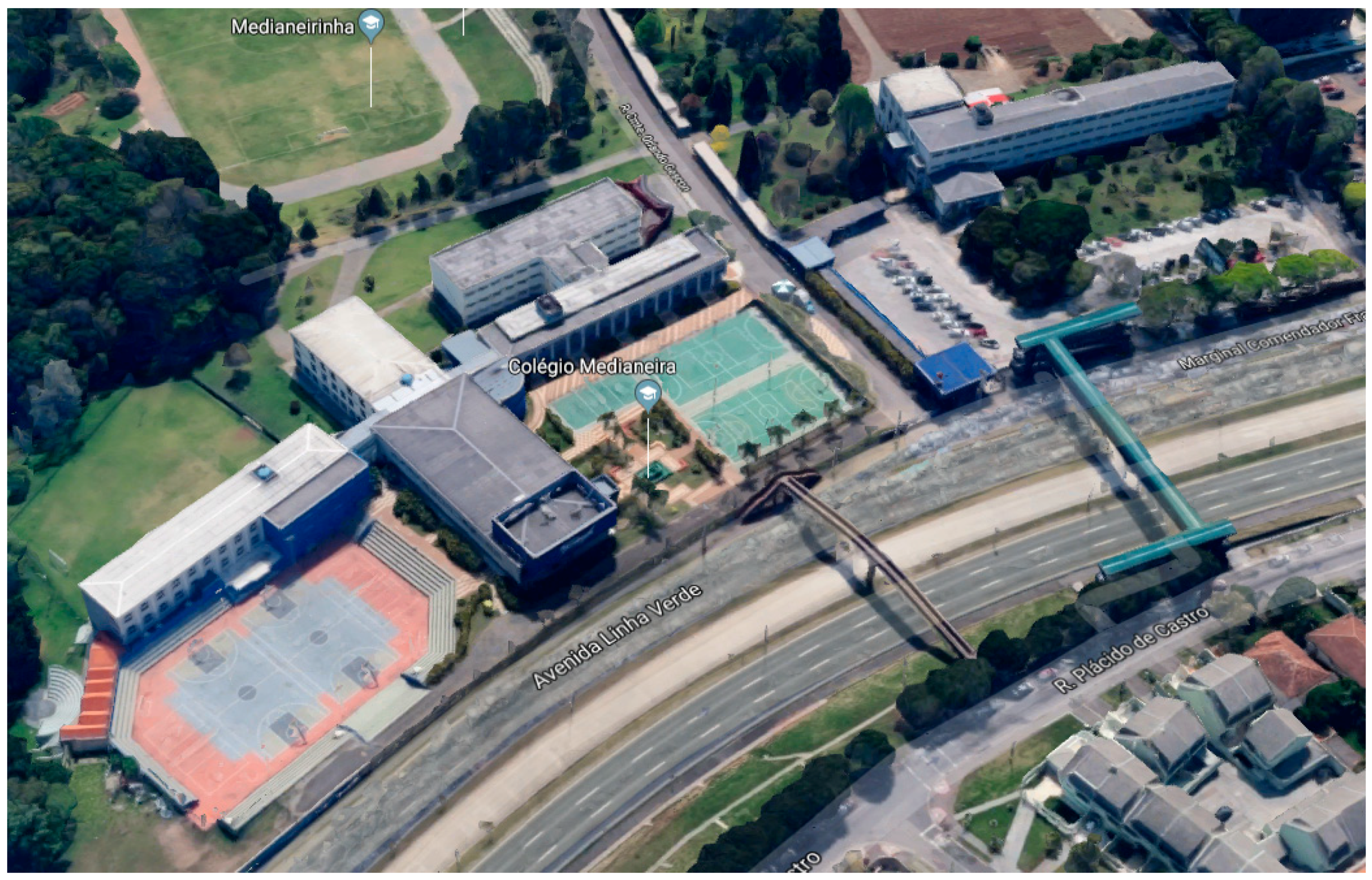
The portion of the highway selected for this study was a flat region without significant gradients. Vehicle traffic was mixed, consisting of motorcycles, light vehicles (cars and utilities), heavy vehicles (trucks and public transport buses). The surroundings of this stretch of the highway contains residential, educational and commercial establishments.

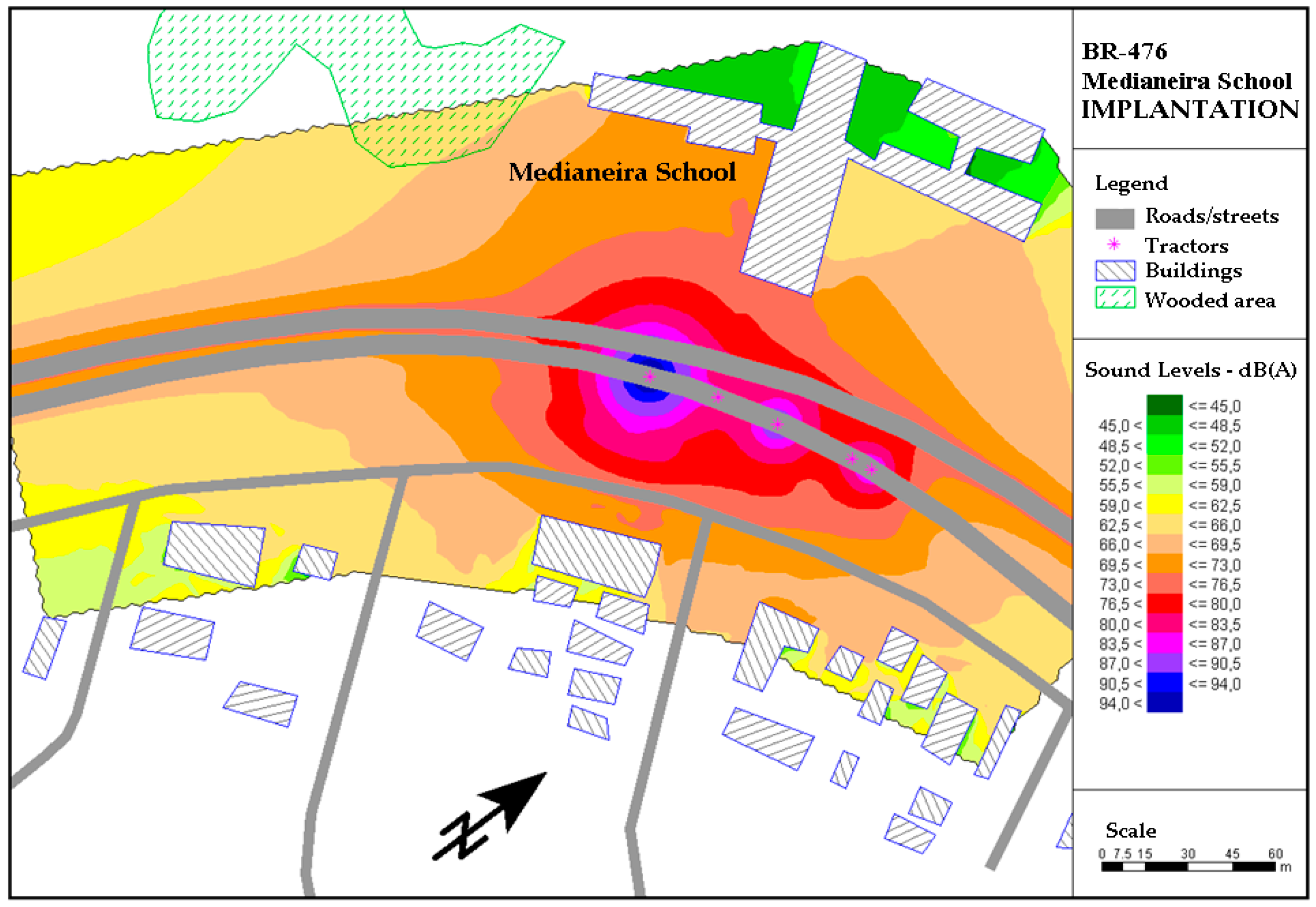
An area of evaluation was chosen within the region selected for analysis, called a “noise-sensitive area,” i.e., an area with educational buildings, where the environmental noise impact assessments were conducted. After the site was chosen, computer simulations were done of the situations of implementation and operation of the highway remodeling project, taking into account all the aforementioned characteristics of the site, using SOUNDPLAN version 6.2 software (SoundPLAN GmbH, Etzwiesenberg, Germany) dedicated exclusively to this type of graphic analysis.

To properly model the real conditions and use them for the simulations with SOUNDPLAN software, the road traffic composition was stratified into cars, heavy vehicles (metropolitan buses, trucks) and light vehicles (motorcycles). Then, after calculating the traffic composition (expressed in percentage), a visual count of vehicles was made independently by two people standing on opposite sides of the road. Road traffic speed was measured by the speedometer of a car driven by two of the authors along this stretch of road, who recorded the average vehicle flow speed, while the other two authors measured the equivalent sound pressure levels in the area.

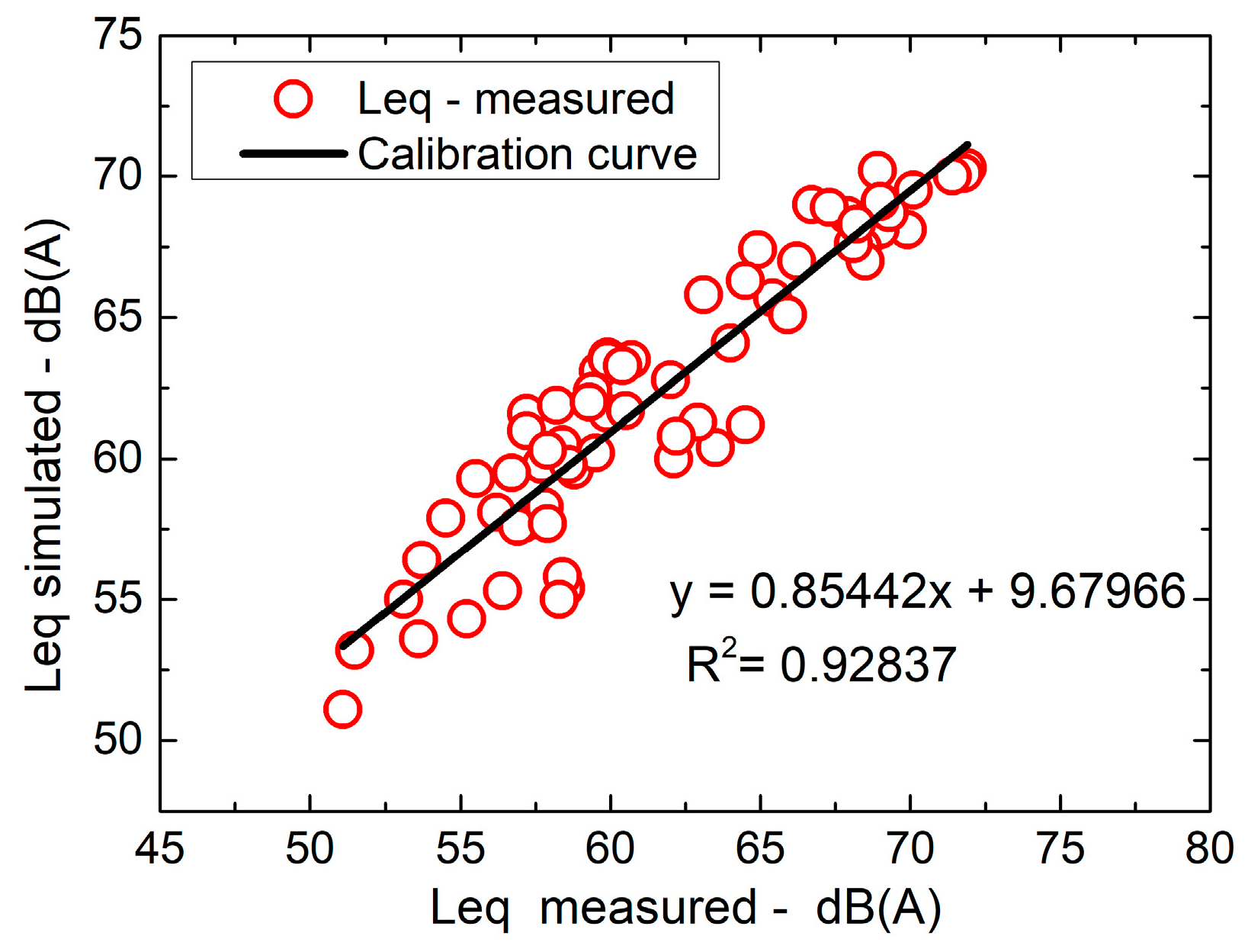
After this assessment of the study area, simulations were made and were validated by comparing the equivalent sound levels of the simulated noise map against the measured road traffic noise emissions. A calibration curve was plotted to compare these values, which were then evaluated based on Pearson’s linear correlation. The results were considered validated when the difference between the measured and simulated values did not exceed ±4.6 dB, as recommended by [37].

A traffic flow of 780 vehicles/h was considered, with 8.5% of the total flow corresponding to heavy vehicles, in the situations of both implementation and operation of the project. The speed considered for both heavy and light vehicles was 40 km/h during the project’s implementation phase.

To determine the environmental impact, an assessment was made of the impact attributes, i.e., classification of the qualitative characteristics of the activity based on the calculated noise maps.

Table 3. Environmental impact attributes pertaining to noise emissions and immissions.

Attribute	Qualification
Phase of occurrence	Implementation (work phase); Operationalization
Area of coverage	Local; Regional
Nature	Positive; Negative
Order	First order (direct source); Second order (indirect source)
Probability of occurrence	Uncertain; Certain
Duration	Short and medium term; Long term; Immediate
Importance	Temporary; Permanent
Possibility of reversal	Minor; Intermediate; Major

lists the attributes in question.

The noise maps for the situation of operationalization were prepared considering the basic project for the Metropolitan Axis of Curitiba’s Integrated Transport Network. This project includes: (1) the prioritization of public transport, with the implementation of express bus-only lanes; (2) frontage roads for the circulation of traffic between different neighborhoods of Curitiba and of metropolitan municipalities; (3) local access roads to reach neighboring activities; and (4) implementation and remodeling of bike paths and green areas. In the operation simulation, double-and triple-articulated buses were considered, passing through at 3-min intervals.

2.4. Design of Experiments

Design of Experiments (DoE) considers the linear effects of certain variables on the outputs of a given system. To this end, most of the significant factors that interfere in the simulated or measured response to a given condition of an experiment are statistically estimated [38]. In this work, therefore, DoE was employed to evaluate the effectiveness of noise barriers designed for the acoustic protection of an educational establishment impacted by high sound pressure levels. The controllable design variables of the noise barriers were the barrier height and the sound absorption coefficient of the barrier material.

The DoE used in this study was a 2^k full factorial design, i.e., with two controllable variables and with k = 2 levels. The levels were raised from the minimum (−1) to the maximum (1). The area of acoustic shadow, with an average level of 55 dB(A), and the sound attenuation calculated from the Transmission Loss (TL) [39] were considered responses and were defined as:

$$\mathrm{TL}=10\times \log (\frac{{10}^{\mathrm{Lr}/10}}{{10}^{\mathrm{Ls}/10}})$$

(1)

where $\mathrm{Lr}$ is the sound pressure level in dB(A) at the receiver position and $\mathrm{Ls}$ is the sound pressure level in dB(A) at the source position.

According to the ASTM C423-17 [40], the absorption coefficient can be represented by the Noise Reduction Coefficient (NRC). The NRC is calculated as the simple average of the absorption coefficient at the frequencies of 250 Hz, 500 Hz, 1000 Hz, and 2000 Hz.

Table 4. Sound absorption coefficients of the noise barriers.

Material *	250 Hz	500 Hz	1000 Hz	2000 Hz	NRC
Smooth Concrete	0.01	0.02	0.02	0.02	0.02
Rockwool	0.50	0.5	0.52	0.60	0.53

(*)—SoundPlan version 6.2 internal library. NRC: Noise Reduction Coefficient.

lists the materials used here: smooth bare concrete and smooth concrete covered with 30 mm rockwool acoustic insulation slabs, with their respective sound absorption coefficients.

Based on a 2² factorial DoE,

Table 5. Coded levels of the factors.

Level	Natural Factors		Coded Factors *
	Barrier Height	NRC	A	B
Minimum	3 m	0.02	−1	−1
Maximum	5 m	0.45	+1	+1

(*)—Coded factors A and B stand for the natural factors barrier height and NRC, respectively.

shows the relationship between natural and coded levels, indicating the factors that are controllable during the design phase. The simulated responses were therefore based on combinations of these two controllable factors.

The controllable coded factors were then arranged in tabular form, called a contrast matrix. This matrix corresponds to the arrangement of all possible combinations of the controllable coded factors between −1 and +1 with an added mean term (M). The output responses were the area of Acoustic Shadow (AS) and Transmission Loss (TL), as indicated in

Table 6. Setup of the contrast matrix for the whole system.

Run	Contrast Input Matrix-X				Output Response Vector–Y
	Mean *	Main Effects		Interaction Effects	Response 1–y1	Response 1–y2
	M	A	B	AB	TL	AS
1	1	−1	−1	1	y11	y21
2	1	1	−1	−1	y12	y22
3	1	−1	1	−1	y13	y23
4	1	1	1	1	y14	y24

(*)—To apply Multiple Linear Regression requires a quadratic matrix to determine the independent regressor (${\mathsf{\beta }}_0$) from $\mathsf{\beta }={({\mathrm{XX}}^{\mathrm{T}})}^{-1}\mathrm{y}$. This explains the presence of the mean term (M) in the column of 1’s. TL: Transmission Loss, AS: Acoustic Shadow.

.

Mathematically, the DoE estimated the effects of the controllable factors on the responses by subjecting the data listed in Table 5 to a multiple linear regression (MLR) [38]. The MLR was applied to each response individually. The significant effects of the input variables on the responses were calculated based on the values of the regressors, which are the ${\mathsf{\beta }}_{\mathrm{j}}$ coefficients shown in Equation (2).

$${\mathrm{y}}_{\mathrm{i}}={\mathsf{\beta }}_0+{\displaystyle \sum _{\mathrm{j}=1}^{\mathrm{k}}}{\mathsf{\beta }}_{\mathrm{j}}{\mathrm{x}}_{\mathrm{ij}}+{\mathsf{ϵ}}_{\mathrm{i}},\mathrm{i}=1,2,\dots ,\mathrm{n}.$$

(2)

In Equation (2) ${\mathrm{x}}_{\mathrm{ij}}$ represents the input of the contrast matrix shown in Table 5, and ${\mathsf{ϵ}}_{\mathrm{i}}$ is the estimation error. On the other hand, Equation (2) can be written in matrix form as $\mathrm{y}=\mathrm{X}\mathsf{\beta }+\mathsf{ϵ}$, thereby allowing the effects to be calculated analytically based on the Least Squares method, establishing the best set of possible regressors, which are calculated as: $\mathsf{\beta }={({\mathrm{XX}}^{\mathrm{T}})}^{-1}\mathrm{y}$, the ${\mathrm{X}}^{\mathrm{T}}$ refers to the matrix transposition operation, the operator ${()}^{-1}$ stands for the inverse matrix operation, and with the $\mathsf{\beta }$ calculated through, $\mathsf{\beta }={({\mathrm{XX}}^{\mathrm{T}})}^{-1}\mathrm{y}$, using the Least Squares method generates the best possible estimations for the response variable, ${\mathrm{y}}_{\mathrm{i}}$ when the $\mathsf{\beta }$ are coupled in Equation (2) [38].

According to Montgomery [38], the nominal effects are calculated as double the values of the regressors, which, in this case, are the ${\mathsf{\beta }}_{\mathrm{j}}$ terms in Equation (2) However, in this work, it was considered the significance of the effects according to the values of the unweighted regressors. This was done to ensure the results would be aligned with those obtained by the neural networks methodology. The codes and computational implementations were performed using Matlab version R2016b software (MathWorks, Natick, MA, USA).

2.5. Artificial Neural Networks

As Haykin et al. [41] proved through the Universal Approximation Theorem [42], Artificial Neural Networks (ANNs), or simply neural networks, are considered universal approximations of functions for structured or unstructured multivariate datasets. ANNs are used in a wide range of fields, such as clustering, prediction, fitting, forecasting, and modeling [43,44]. ANNs learn and recognize the dynamics of a given system through the dichotomy of input-output pairing. With this, one can establish the heuristic of supervised machine learning based on error backpropagation, which is calculated as the difference between the output estimated by the network and the target value. By means of training algorithms, this error determines the direction and speed of learning. For in-depth details of neural network concepts, see Haykin et al. [41] and Russell et al. [45].

In this work, the ANNs were implemented based on the Multilayer Perceptron (MLP) architecture, with a topology of one input layer, two hidden layers, and one output layer. Six topologies were trained for each response variable in order to avoid biased terms, as indicated in

Table 7. Setup of the artificial neural networks (ANNs) topologies.

Descriptor	Setups Used in This Work
Architecture	Multilayer Perceptron
Training method	Supervised
Topology 1	3-5-5-1
Topology 2	3-10-10-1
Topology 3	3-15-15-1
Topology 4	3-20-20-1
Topology 5	3-25-25-1
Topology 6	3-30-30-1
Training algorithm	Error backpropagation with Levenberg-Marquardt
Activation Functions on the 1° e 2° hidden layers	Hyperbolic tangent
Activation function on output layer	Linear Function

.

The input layer of the network contained three sensory neurons corresponding to the variables defined in the DoE, i.e., barrier height, the barrier’s NRC, and the interaction between the two, which corresponds to the coded variables A, B and AB. The size of the ANN training topologies was chosen to perform the approximation with only one neuron in the output layer. In other words, for each of the y₁ and y₂ responses listed in Table 6, a specialized neural network was trained with only 1 neuron in the output layer. Table 7 shows the configuration of the ANNs that were trained.

Due to the small number of samples available for ANN training, it was employed the heuristic for the training phase recommended by Hinton et al. [46]. The samples were therefore divided as follows: 90% of the samples were used for training and 10% for validation and testing, arranged in a cross-validation scheme using Matlab defaults. These samples were allocated randomly. The input-output pairs were subjected to bipolar normalization in a range of −1 to 1, enabling us to prevent possible scaling effects from masking the real factors of significance. This mapping, which was performed in the DoE and ANNs as a preprocessing phase prior to applying the MLR, is expressed by Equation (3):

$$\mathrm{y}=({\mathrm{y}}_{\max }-{\mathrm{y}}_{\min })·\frac{(\mathrm{x}-{\mathrm{x}}_{\min })}{({\mathrm{x}}_{\max }-{\mathrm{x}}_{\min })}+{\mathrm{y}}_{\max }$$

(3)

In Equation (3) $\mathrm{x}$ represents the variable to be mapped between −1 and 1, the minimum and maximum values of $\mathrm{x}$ are, respectively, ${\mathrm{x}}_{\min }$ and ${\mathrm{x}}_{\max }$, and ${\mathrm{y}}_{\min }$ = −1 and ${\mathrm{y}}_{\max }$ = 1. The training stopping criteria were the normalized Mean Square Error (MSE) of 1 and −12, a maximum of 500 epochs, and a limit training time of 5 min.

The performance criteria used were the normalized Mean Square Error (MSE) and Pearson’s linear correlation ($\mathrm{R}$) between the estimated output and the target output. The MSE was calculated in the context of the ANNs as:

$$\mathrm{MSE}=\frac{1}{2\mathrm{N}}{\displaystyle \sum _{\mathrm{n}=1}^{\mathrm{N}}\sum _{\mathrm{j}\in \mathrm{C}}}{\mathrm{e}}_{\mathrm{j}}^2(\mathrm{n})$$

(4)

In Equation (4) the error is:

$${\mathrm{e}}_{\mathrm{j}}(\mathrm{n})={\mathrm{d}}_{\mathrm{j}}(\mathrm{n})-{\mathrm{y}}_{\mathrm{j}}(\mathrm{n})$$

(5)

The subscript $\mathrm{j}$ indicates that this is the network’s output layer. The error ${\mathrm{e}}_{\mathrm{j}}$ was calculated as the difference between the real value of the network’s output ${\mathrm{d}}_{\mathrm{j}}(\mathrm{n})$, and the ${\mathrm{y}}_{\mathrm{j}}(\mathrm{n})$ value estimated by the network, considering a total number of samples of $\mathrm{N}=4$. The level of Pearson’s linear correlation $(\mathrm{R})$ between ${\mathrm{d}}_{\mathrm{j}}(\mathrm{n})$ and ${\mathrm{y}}_{\mathrm{j}}(\mathrm{n})$ is:

$$\mathrm{R}=\frac{{\sum }_{\mathrm{j}}^{\mathrm{N}}({\mathrm{d}}_{\mathrm{j}}-\overline{\mathrm{d}})({\mathrm{y}}_{\mathrm{j}}-\overline{\mathrm{y}})}{(\mathrm{N}-1){\mathrm{s}}_{\mathrm{d}}{\mathrm{s}}_{\mathrm{y}}}$$

(6)

and the components of Equation (6) are:

$${\mathrm{s}}_{\mathrm{d}}=\sqrt{\frac{1}{\mathrm{N}-1}{\displaystyle \sum _{\mathrm{n}=1}^{\mathrm{N}}}({\mathrm{d}}_{\mathrm{n}}-\overline{\mathrm{d}})};{\mathrm{s}}_{\mathrm{y}}=\sqrt{\frac{1}{\mathrm{N}-1}{\displaystyle \sum _{\mathrm{n}=1}^{\mathrm{N}}}({\mathrm{y}}_{\mathrm{n}}-\overline{\mathrm{y}})}$$

(7)

where the terms ${\mathrm{s}}_{\mathrm{d}}$ and ${\mathrm{s}}_{\mathrm{y}}$ are respectively the standard deviation for the output ($\mathrm{d}$) and to the target ($\mathrm{y}$).

Equation (6) therefore tells us how aligned the estimated errors are in their variances. In this work, the level of correlation between the outputs was R². This is the most important metric to be evaluated when comparing the performance of the ANNs and the DoE.

To obtain an optimized response for the various training sessions of the neural network, a mean equivalent neural network, (ANN_eq)_mean, was calculated for each topology. The following steps were carried out:

(i)

50 independent training sessions were performed for each topology shown in Table 7. The spatial weights matrix was reset to zero in each new training session. The normalized mean square error (MSE) training performance indicator of each training session was stored as MSE(i), with i = 1 up to 50.

(ii)

The simple average of the set of 50 MSE values corresponding to the training session of the previous step was calculated for each of the 5 topologies shown in Table 6. This average value was calculated as: ${\mathrm{MSE}}_{\mathrm{mean}}=(1/50){\sum }_{\mathrm{i}=1}^{50}\mathrm{MSE}(\mathrm{i}).$

(ii)

It was checked whether the MSE(i) of each of the 50 trained neural networks was greater than the MSE_mean value. If the MSE(i) < MSE_mean, then this MSE(i) network was added to the new optimized MSE_opt set.

(iv)

The simple average of this new MSE_opt set was calculated, thus generating the (ANN_eq)_mean.

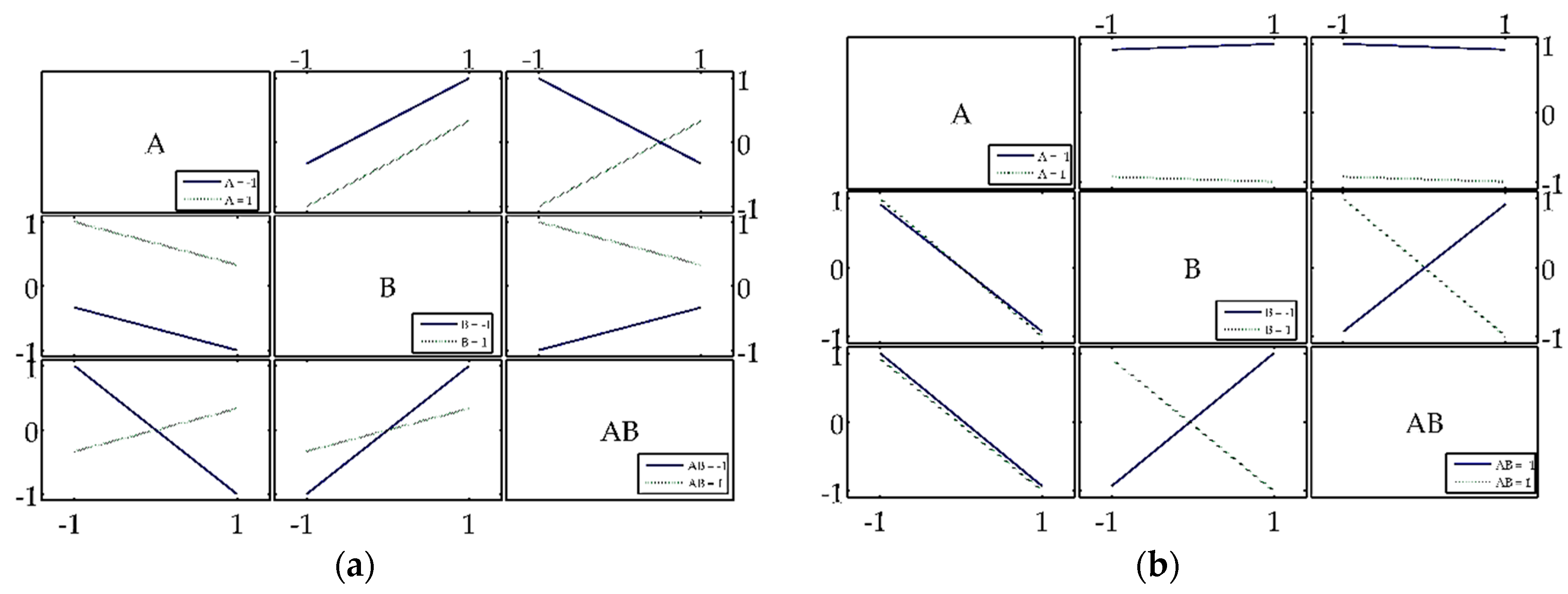
In this work, it was employed the modified version of the Profile Method (PM) [47,48], hereinafter referred to as the Modified Profile Method (MPM), which was successfully applied by Nascimento and Oliveira [49] and by Nascimento et al. [50]. According to Lek et al. [47], the original PM calculated the profile curves of each variable. A profile curve can be understood as a curve which contains the scale of the variable on the abscissa axis, i.e., the number of discrete points to which the input variable is segmented within its range, from its minimum to its maximum. Thus, the independent variable is calculated considering the average of five points applied at the output of the trained neural network. These points are the minimum value, the 1st, 2nd, and 3rd quartiles and the maximum value. As a function of the scale, the resulting curve is called the profile curve that corresponds to the input variable.

The MPM therefore calculates the significance of a given input variable of the ANN by subjecting the optimized profile curve to a linear regression. In addition, as explained earlier herein, six topologies, each trained 50 times, were considered, from which an optimized equivalent mean neural network, (ANN_eq)_mean, was derived. In contrast, the original PM calculates the significance based only on the maximum value of the profile curve for each input variable.

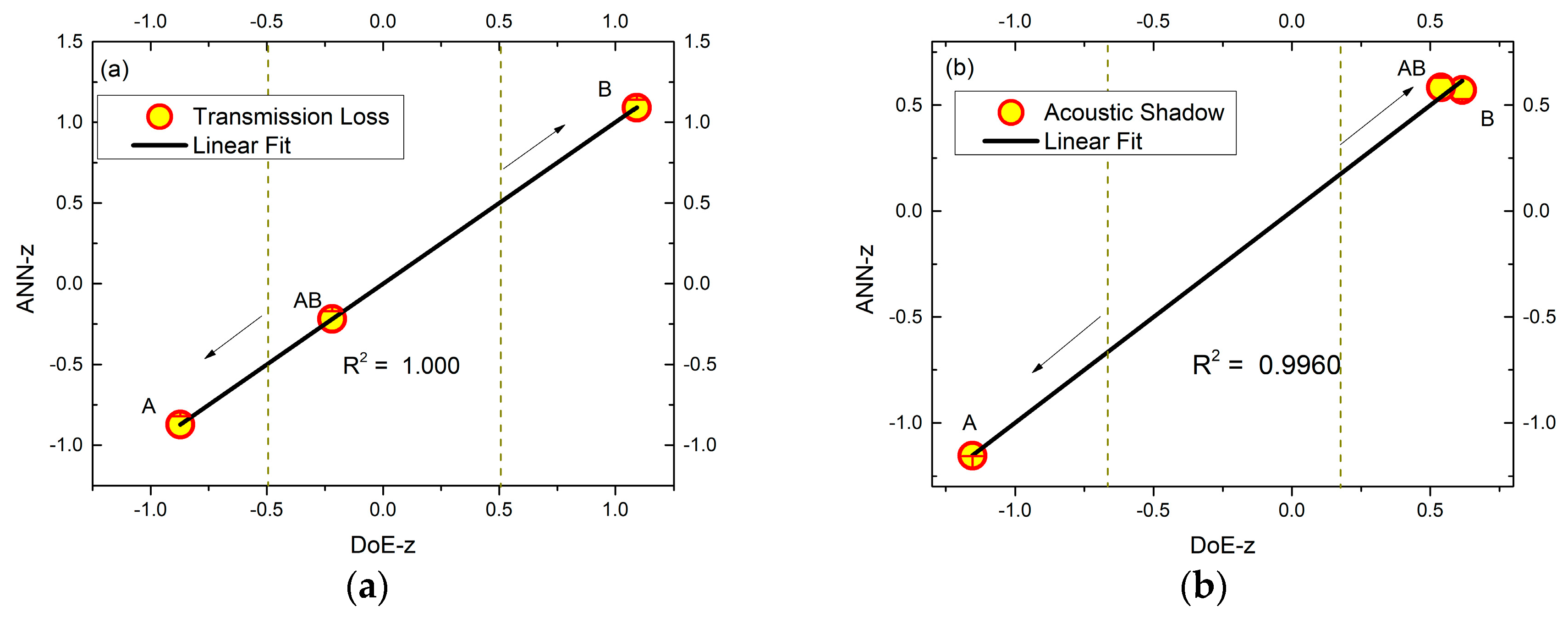
In order to make a proper graphical comparison of the performances and estimate the significance of the controllable factors, the results of the ANN and DoE regression coefficients were normalized to ANN-z and DoE-z. This normalized transformation of the data on the z-scale weighs the residual difference of the estimators based on their standard deviation, as shown in Equation (8).

$$\mathrm{z}=\frac{(\mathrm{x}-\overline{\mathrm{x}})}{\mathrm{S}}$$

(8)

The standard deviation (S) for a random population is:

$$\mathrm{S}=\sqrt{\frac{1}{\mathrm{P}-1}{\displaystyle \sum _{\mathrm{i}=1}^{\mathrm{P}}}{({\mathrm{x}}_{\mathrm{i}}-\overline{\mathrm{x}})}^2}$$

(9)

where $\mathrm{P}$ is the number of regressors, in this case corresponding to A, B and AB, which generates $\mathrm{P}$ = 4 in Equation (9), while ${\mathrm{x}}_{\mathrm{i}}$ corresponds to the samples of the controllable factors, as indicated in Table 4.

3. Results and Discussion

The results were divided into two steps: (i) comparison and evaluation of environmental impacts on Medianeira School in the following scenarios: current, implementation, and operationalization; and (ii) study of the evaluation of the significant effects of noise barrier designs applying the DoE and the ANNs.

3.1. Assessment Results

The noise maps generated by computer simulation for the various phases of the project, i.e., current, implementation, and operationalization, are shown below. The maps are presented sequentially, preceded by information about their main identified features. The classification of noise pollution was formulated for a mixed area of approximately 20 km², according to Curitiba Municipal Law No. 10625 [35] and the Brazilian standard NBR-10151 [34] Noise Assessment in Communities, in terms of acceptable percentages: from 0% to 20%—clearly polluted; from 21% to 50%—partially polluted, from 51% to 70%—slightly polluted, and from 71% to 100%—ideal.

Current Situation

Noise levels in the surroundings of the highway of 74–76 dB(A). Existence of concentrated areas along the highway in the range of 76–78 dB(A) due to the reduction of the highway lane divider between main roads. Existence of a potentiated zone of 72–74 dB(A) between the main lanes of the highway due to the existence of an unpaved embankment dividing these lanes. Noise levels of 66–68 dB(A) at the facades of buildings situated along the road, and of 62–64 dB(A) at the facades of buildings situated further back from the road. Presence of an educational establishment with noise levels of 66–68 dB(A) at its main façade, Figure 1.

Most of this stretch of the highway is not in compliance with the legal requirements for acceptable daytime noise levels, as can be seen in

Table 8. Comparison of maximum acceptable values, current situation, daytime.

Legislation and Standards	Period	Maximum Value [dB(A)]	% Compliance	Acoustic Situation
Law No. 10625 (SZ-BR-476–special zone of BR-476)	Daytime	65	16	Clearly polluted
Law No. 10625 (SEZ–special educational zone)	Daytime	60	0	Clearly polluted
NBR-10151 standard (mixed zone)	Daytime	65	16	Clearly polluted
NBR-10151 (with special buildings)	Daytime	55	0	Clearly polluted

.

In the current situation, the noise levels already exceed the maximum permissible Leq of 65 dB(A).

3.2. Implementation Phase

Most of this stretch of the highway is not in compliance with the legal requirements for acceptable daytime noise levels, as indicated in

Table 9. Comparison of maximum acceptable values, implementation phase, daytime.

Legislation and Standards	Period	Maximum Value [dB(A)]	% Compliance	Acoustic Situation
Law No. 10625 (SZ-BR-476–special zone of BR-476)	Daytime	65	13	Clearly polluted
Law No. 10625 (SEZ–special educational zone)	Daytime	60	0	Clearly polluted
NBR-10151 standard (mixed zone)	Daytime	65	13	Clearly polluted
NBR-10151 (with special buildings)	Daytime	55	0	Clearly polluted

.

Noise levels in the order of 90.5 dB(A) to 94 dB(A) in the vicinity of the points representing earthmoving equipment (graders and backhoes), with one concentrated area. Job site noise levels range from 76.5 dB(A) to 94 dB(A). Noise levels in the range of 73–76.5 dB(A) at the facades of buildings along the highway, and of 66–73 dB(A) at the facades of buildings further back from the highway. Presence of an educational establishment with noise levels in the range of 73–76.5 dB(A) at its front façade, Figure 2.

Continuous exposure to noise levels of this magnitude can give rise to psychological and physiological problems [12,17].

3.3. Operationalization Phase

For this phase, only the limit values for zones with buildings for special uses were considered, because after the project is completed, this urban stretch of highway will become a municipal road and will fit the category of a special educational zone (SEZ—Special Zones). Continuous noise levels in the range of 72–74 dB(A) are expected in the proximities of the urban avenue.

Table 10. Comparison of maximum acceptable values, operationalization phase, daytime.

Legislation and Standards	Period	Maximum Value [dB(A)]	% Compliance	Acoustic Situation
Curitiba Law No. 10625 (SEZ)	Daytime	60	13	Clearly polluted
NBR-10151 (with special buildings)	Daytime	55	0	Clearly polluted

shows the levels of operationalization.

The operationalization of the road urbanization project will intensify the existing noise pollution levels. Noise levels in the range of 68–70 dB(A) are expected at the facades of buildings along the avenue, and of 62–64 dB(A) at the facades of buildings further back from it. Noise levels in the range of 68–70 dB(A) were simulated at the front façade of an educational establishment, Figure 3.

This stretch of the highway is not in compliance with the legally permissible daytime noise levels, as indicated in Table 9.

3.4. Environmental Impact Matrix

Table 11. Environmental Impact Matrix of the Implementation and Operationalization phases.

Attribute	Qualification
Phase of occurrence	Implementation	Operationalization
Area of coverage	Local	Local
Nature	Negative	Negative
Order	First order	First order
Probability of occurrence	Certain	Certain
Beginning	Immediate	In the short term
Duration	Temporary	Permanent
Importance	Major	Major
Possibility of reversal	Reversible	Reversible

describes the Environmental Impact Matrices of the implementation and operationalization phases of the project in terms of measured and simulated noise levels.

The results of the impact matrix indicate potentially reversible situations.

3.5. Significance Analysis of the Design of Noise Barriers–A Qualitative Approach

The area where the “educational establishment” is located receives road traffic noise from the highway that passes in front of it. For the simulations described below, a noise barrier was demarcated measuring 152 m at the front, 92 m on the right-hand side and 78 m on the left hand side. The barrier is marked off by the white line in Figure 4.

Figure 5 shows the calibration curve of the current situation. The measured and simulated noise levels showed a strong linear correlation of R² = 0.928. It should also be noted that the greatest absolute difference between the measured and simulated noise levels was 3.3 dB(A), which is in line with the condition that the difference should not exceed ±4.6 dB(A).

Based on the validated simulations of the current condition (see Figure 5), noise barriers were simulated in several conditions, by varying their height and the material of which they were made.

Figure 6 shows the noise map of the current situation of noise immissions that reach the front facade of Medianeira School. Clearly visible are the high noise levels that reach the classrooms facing the highway, with sound levels ranging from 67 to 70 dB(A) or even higher, characterizing a situation of serious noise pollution, according to the attributes of the environmental impact matrix listed in Table 8.

In an attempt to reduce these high noise levels, acoustic simulations were made using noise barriers of different materials and heights. Thus, Figure 7a, for example, shows the noise map calculated for a 3 m high raw concrete noise barrier. As can be seen, the sound levels decrease from 70 dB(A) to 67 dB(A), to 64 dB(A), and so on until they reach 61 dB(A) at the front of the school. Another important point is that the size of the acoustic shadow-green color behind the school increased. With the 5 m high raw concrete noise barrier, the acoustic shadow, whose sound levels are lower than 55 dB(A), is much larger than without the presence of the barrier. Therefore, this noise reduction measure indicates that the problem is reversible, according to the attributes listed in Table 7. However, despite the reduction in noise levels, they are still not in compliance with the 60 dB(A) limit established by municipal legislation nor the 55 dB(A) limit established by the Brazilian standard NBR 10151 [34].

The noise map in Figure 7b illustrates the acoustic situation simulated with a 5 m high raw concrete noise barrier. In this situation, the noise levels in the outermost parts of the school are already acceptable according to Curitiba municipal legislation, i.e., below 65 dB(A). The sound levels in this area range from 58 to 61 dB(A). Also note that the entire front facade of the school, further back, presents sound levels in the order of 55 to 58 dB(A)—yellow color.

Therefore, the municipal legislation is fully met, and it is proven that the noise problem pointed out in Table 8 is reversible. The reduction in noise levels was in the order of 70 dB(A) to 55 dB(A), i.e., a noise reduction of 15 dB(A) was achieved, satisfying the municipal legislation and the Brazilian standard for noise assessment in communities, as described in Table 4. The noise limit established by municipal legislation for Special Educational Zones—SEZ is 60 dB(A) and that established by the Brazilian standard NBR 10151 for Educational Zones is 55 dB(A).

3.6. Significance Analysis of the Design of Noise Barriers—Quantitative Approach

The DoE and MPM methodologies were applied to reinforce the evaluation of the significance of the controllable factors in the noise barrier designs. Initially, the results were presented separately. Emphasis was placed on specific discussions to highlight the advantages of these new types of solutions for the optimum design of noise barriers aimed at mitigating the harmful effects of noise pollution.

3.6.1. Significance Analysis Using DoE

Figure 6 illustrates the results of the acoustic mapping described by the factors listed in Table 5. In the quantitative bias,

Table 12. Contrast matrix of the overall system.

Run	Run Order	Mean	Main Effects		Interaction Effect	Response
		M	A	B	AB	TL	AS—m2
1	2	1	−1	−1	1	6	76,551
2	1	1	1	−1	−1	3	67,063
3	4	1	−1	1	−1	12	76,976
4	3	1	1	1	1	9	66,920

lists the values of the equivalent responses for each of the cases of the combinations established in the DoE and described in Table 6.

Figure 8 shows 12 graphs of the paired interactions between the controllable factors and their impacts on the outputs of the system under study, namely, Transmission Loss, TL, and acoustic shadow, AS. This figure shows which of the controllable factors of the barrier designs, that is, variables A, B and AB, have the strongest impact on the increase or decrease of the system’s outputs, TL and AS. In Figure 8, note that there is a concordance in the behavior of the two responses TL and AS. Hence, the analysis of Figure 8a applies to Figure 8b.

Figure 8a evaluates the TL factor. Factors A and B were found to be independent of each other, so the main effects of one do not interact with the responses of the other, and vice versa, as indicated by the highly parallel lines. In contrast, the effect of the “AB” regressor interacts with responses A or B, increasing or decreasing them, as indicated by the non-parallel lines in the third row and in the third column.

This enabled us to determine that, in general, factor B was correlated with the increase in TL, indicating that, in terms of acoustic protection, the ideal noise barrier designs are those with high noise reduction coefficients (NRC) and taller heights. To validate the estimates of significance of the effects on the linear models, the values of R² = 0.7454 and R² = 0.9621 were obtained for TL and AS, respectively.

3.6.2. Significance Analysis Using ANNs

Table 13. Results and optimization of ANN performance.

Qualifiers	Topologies
	1	2	3	4	5	6
ANN*	50	50	50	50	50	50
(ANNeq)mean	34	34	30	29	30	33
MSE*	7.13	7.92	8.40	6.15	6.94	6.72
(MSEeq)mean	4.17	3.08	1.82	1.32	1.23	4.48
R2	0.88	0.74	0.71	0.90	0.70	0.67
(R2eq)mean	0.99	0.96	1.00	1.00	0.99	0.80

*Artificial Neural Networks (ANN), Mean Squared Normalized Error (MSE).

describes the results achieved in training performance after the optimization proposed in Section 2.5. Note that of the 50 topologies initially trained, only 31 were subjected to the MPM. Also note the lower (MSE_eq)_mean values after optimization than those of the networks without MSE optimization. Moreover, after optimization, the Pearson R² correlation levels (R²_eq)_mean were close to 1, whereas before the optimization the mean value was 0.73.

Figure 9 shows an example of the significance calculated by applying the MPM and its respective linear regression, which will indicate the significance of factor A in the responses of TL and AS.

The results shown in Table 13 and in Figure 9 therefore validate the use of the MPM.

3.6.3. Comparison of DoE and ANN

The regressors for each of the methodologies of the DoE and ANN are shown in

Table 14. Comparison of the results of the effects of significance applying ANN and Design of Experiments (DoE).

Qualifiers	Medianeira School				z-Score Results				Error in z-Score
	TL		AS		TL		AS		TL	AS
	DoE	ANN	DoE	ANN	DoE	ANN	DoE	ANN	DoE	ANN
A	−1.50	−0.91	−4943	−2274.33	−0.87	−0.87	−1.16	−1.16	0%	−0.07%
B	3.00	1.70	13.50	−218.17	1.09	1.09	0.62	0.57	0%	7.74%
AB	0.00	0.16	−199.00	−203.63	−0.21	−0.21	0.54	0.58	0%	−7.72%

. This table shows, in condensed form, the comparisons of the regressors on the z-score scale.

Based on Table 14, it can be seen that, on the z-score scale, the errors for the estimated values applying the DoE and ANNs show minor deviations. The use of the z-score standardizes the results, since the qualitative result of the z-score enables estimates to be made without biased terms augmented by amplitude factors. Thus, one can see that, in general, the two methodologies produce concordant results insofar as they find that factors A and B are the most significant.

The relative dispersion of significance and comparison of the accuracy of estimated effects are plotted in Figure 10. The regression line shows a high correlation, R² = 0.9995, obtained by the regression of DoE-z versus ANN-z. Thus, the points in the graphs of Figure 10 which are farthest away from the source correspond to the strongest impacts on the response. Figure 10b therefore clearly indicates that the significance of the coded interaction factor AB is low when compared to factors A and B, which is the same result as that obtained by the DoE. This finding is in agreement with the literature, as shown by Montgomery [38], that the magnitude of the interaction effects are generally lower.

From the mathematical standpoint, the results presented here are in full agreement with the literature, above all in that the amplitudes of the interaction factors are in line with the expected values [38]. On the other hand, an environmental analysis of the results highlights the following two factors. (i) Noise barrier height, in every case, is shown to be the most significant parameter, directly enhancing the mitigation of sound pressure levels in front of and behind the barrier. (ii) The absorption coefficients of noise barrier materials are particularly important, because they indicate whether the barrier will create acoustic scattering that tends more towards reflection or more towards sound absorption.

4. Conclusions

The results provided by the ANNs were in good agreement with those obtained by the DoE. The largest error found in the z-score for the estimators A, B, and AB, including the rankings for the two response variables TL and AS, was 7.72%. On the other hand, the correlations between the DoE-z and ANN-z significance of ranking for the TL and AS responses were, respectively, R² = 0.99887 and R² = 0.9877. Thus, for each response variable (TL and AS), the ANN-z and the DoE-z revealed the same ranking, i.e., in order of significance: B, A and AB for the response variable TL, and A, B, and AB for the response variable AS. Thus, the results conclusively indicated that the TL of an acoustic barrier is more strongly influenced by the absorption coefficient of the barrier than by its height, while the AS is more influenced by the height of the barrier than by its absorption coefficient. These results are extremely relevant, since the ANNs used here had not been taught the physics required to calculate sound absorption and sound attenuation. The results were thus obtained based on only the system’s input and output data, indicating the independent linearity given by the non-parameterization of the variables. This method for significance testing using ANNs can be extrapolated to other areas of environmental acoustics and noise control.

The implementation and operationalization of the road urbanization project will intensify the existing noise pollution, resulting in a negative local environmental noise impact. The magnitude of this impact in terms of increased noise levels represents an unhealthy condition for the population living or working along this avenue or in its proximities. Therefore, in a region where the noise levels already exceed the legal limits, this increase is considered to pose a risk, requiring the immediate adoption of mitigating measures, which should be defined early in the project’s design phase. It should also be kept in mind that this region includes a “sensitive” area, i.e., an “educational establishment,” which must be protected against high noise levels.

The simulations clearly show that the noise pollution around the school can be reverted to comply with Curitiba municipal law, with sound levels below 60 dB(A), i.e., around 55 to 58 dB(A), according to the requirements of the environmental impact matrix described in Table 9. With the adoption of the noise barrier depicted in Figure 8, the requirements of the Brazilian standard NBR 10151, which limits noise levels in the surroundings of educational areas to 55 dB(A), were also satisfied. The analysis of significance was suitable for use in the design of noise barriers, serving as an interesting tool for designers to better focus their resources on the variables that actually determine the effectiveness of noise barriers.

References

1. Licitra, G.; Fredianelli, L.; Petri, D.; Vigotti, M.A. Annoyance evaluation due to overall railway noise and vibration in Pisa urban areas. Sci. Total Environ. 2016, 568, 1315–1325. [Google Scholar] [CrossRef] [PubMed]
2. Bunn, F.; Zannin, P.H.T. Assessment of railway noise in an urban setting. Appl. Acoust. 2006, 104, 16–23. [Google Scholar] [CrossRef]
3. Gagliardi, P.; Fredianelli, L.; Simonetti, D.; Licitra, G. ADS-B System as a Useful Tool for Testing and Redrawing Noise Management Strategies at Pisa Airport. Acta Acust. United Acust. 2017, 103, 543–551. [Google Scholar] [CrossRef]
4. Iglesias-Merchan, C.; Diaz-Balteiro, L.; Soliño, M. Transportation planning and quiet natural areas preservation: Aircraft overflights noise assessment in a National Park. Transp. Res. D 2015, 41, 1–12. [Google Scholar] [CrossRef]
5. Kephalopoulos, S.; Paviotti, M.; Anfosso-Lédée, F.; Van Maercke, D.; Shilton, S.; Jones, N. Advances in the development of common noise assessment methods in Europe: The CNOSSOS-EU framework for strategic environmental noise mapping. Sci. Total Environ. 2014, 482, 400–410. [Google Scholar] [CrossRef] [PubMed]
6. Morel, J.; Marquis-Favre, C.; Gille, L.A. Noise annoyance assessment of various urban road vehicle pass-by noises in isolation and combined with industrial noise: A laboratory study. Appl. Acoust. 2016, 101, 47–57. [Google Scholar] [CrossRef]
7. Schmidt, J.H.; Klokker, M. Health effects related to wind turbine noise exposure: A systematic review. PLoS ONE 2014, 9, e114183. [Google Scholar] [CrossRef]
8. Michaud, D.S.; Feder, K.; Keith, S.E.; Voicescu, S.A.; Marro, L.; Than, J.; Guay, M.; Denning, A.; McGuire, D.A.; Bower, T.; et al. Exposure to wind turbine noise: Perceptual responses and reported health effects. J. Acoust. Soc. Am. 2016, 139, 1443–1454. [Google Scholar] [CrossRef] [Green Version]
9. Ruiz-Padillo, A.; Ruiz, D.P.; Torija, A.J.; Ramos-Ridao, Á. Selection of suitable alternatives to reduce the environmental impact of road traffic noise using a fuzzy multi-criteria decision model. Environ. Impact Assess. 2016, 61, 8–18. [Google Scholar] [CrossRef] [Green Version]
10. Khan, J.; Ketzel, M.; Kakosimos, K.; Sørensen, M.; Jensen, S.S. Road traffic air and noise pollution exposure assessment–A review of tools and techniques. Sci. Total Environ. 2018, 634, 661–676. [Google Scholar] [CrossRef]
11. Giles-Corti, B.; Vernez-Moudon, A.; Reis, R.; Turrell, G.; Dannenberg, A.L.; Badland, H.; Foster, S.; Lowe, M.; Sallis, J.F.; Stevenson, M.; et al. City planning and population health: A global challenge. Lancet 2016, 388, 2912–2924. [Google Scholar] [CrossRef]
12. Basner, M.; Babisch, W.; Davis, A.; Brink, M.; Clark, C.; Janssen, S.; Stansfeld, S. Auditory and non-auditory effects of noise on health. Lancet 2014, 383, 1325–1332. [Google Scholar] [CrossRef] [Green Version]
13. Cassina, L.; Fredianelli, L.; Menichini, I.; Chiari, C.; Licitra, G. Audio-Visual Preferences and Tranquillity Ratings in Urban Areas. Environments 2018, 5, 1. [Google Scholar] [CrossRef]
14. Miedema, H.M.; Oudshoorn, C.G. Annoyance from transportation noise: Relationships with exposure metrics DNL and DENL and their confidence intervals. Environ. Health Perspect. 2001, 109, 409–416. [Google Scholar] [CrossRef] [PubMed]
15. Sygna, K.; Aasvang, G.M.; Aamodt, G.; Oftedal, B.; Krog, N.H. Road traffic noise, sleep and mental health. Environ. Res. 2014, 131, 17–24. [Google Scholar] [CrossRef]
16. Minichilli, F.; Gorini, F.; Ascari, E.; Bianchi, F.; Coi, A.; Fredianelli, L.; Licitra, G.; Manzoli, F.; Mezzasalma, L.; Cori, L. Annoyance Judgment and Measurements of Environmental Noise: A Focus on Italian Secondary Schools. Int. J. Environ. Res. Public Health 2018, 15, 208. [Google Scholar] [CrossRef] [PubMed]
17. Vienneau, D.; Schindler, C.; Perez, L.; Probst-Hensch, N.; Röösli, M. The relationship between transportation noise exposure and ischemic heart disease: A meta-analysis. Environ. Res. 2015, 138, 372–380. [Google Scholar] [CrossRef]
18. Fiedler, P.E.K.; Zannin, P.H.T. Evaluation of noise pollution in urban traffic hubs—Noise maps and measurements. Environ. Impact Assess. Rev. 2015, 51, 1–9. [Google Scholar] [CrossRef]
19. Paneto, G.G.; de Alvarez, C.E.; Zannin, P.H.T. Relationship between urban noise and the health of users of public spaces—A case study in Vitoria, ES, Brazil. J. Build. Constr. Plan. Res. 2017, 5, 45. [Google Scholar] [CrossRef]
20. Paiva, K.M.; Cardoso, M.R.A.; Zannin, P.H.T. Exposure to road traffic noise: Annoyance, perception and associated factors among Brazil’s adult population. Sci. Total Environ. 2019, 650, 978–986. [Google Scholar] [CrossRef]
21. Da Paz, E.C.; Zannin, P.H.T. Urban daytime traffic noise prediction models. Environ. Monit. Assess. 2010, 163, 515–529. [Google Scholar] [CrossRef] [PubMed]
22. Bunn, F.; Zannin, P.H.T. Urban planning-Simulation of noise control measures. Noise Control Eng. J. 2015, 63, 1–10. [Google Scholar] [CrossRef]
23. Zannin, P.H.T.; De Sant’ana, D.Q. Noise mapping at different stages of a freeway redevelopment project—A case study in Brazil. Appl. Acoust. 2011, 72, 479–486. [Google Scholar] [CrossRef]
24. Li, T.; Burdisso, R.; Sandu, C. Literature review of models on tire-pavement interaction noise. J. Sound Vib. 2018, 420, 357–445. [Google Scholar] [CrossRef]
25. Zaibi, M.; Cherif, H.; Champenois, G.; Sareni, B.; Roboam, X.; Belhadj, J. Sizing methodology based on design of experiments for freshwater and electricity production from multi-source renewable energy systems. Desalination 2018, 446, 94–103. [Google Scholar] [CrossRef]
26. Jacyna, J.; Kordalewska, M.; Markuszewski, M.J. Design of Experiments in metabolomics-related studies: An overview. J. Pharm. Biomed. 2018, 164, 598–606. [Google Scholar] [CrossRef] [PubMed]
27. Yongfan, L.; Shuai, Z.; Jing, W. Research on the Optimization Design of Motorcycle Engine Based on DOE Methodology. Procedia Eng. 2017, 174, 740–747. [Google Scholar] [CrossRef]
28. Shahsavari, M.H.; Khamehchi, E. Optimum selection of sand control method using a combination of MCDM and DOE techniques. J. Pet. Sci. Eng. 2018, 171, 229–241. [Google Scholar] [CrossRef]
29. Nourani, V.; Fard, M.S. Sensitivity analysis of the artificial neural network outputs in simulation of the evaporation process at different climatologic regimes. Adv. Eng. Softw. 2012, 47, 127–146. [Google Scholar] [CrossRef]
30. Fischer, A. How to determine the unique contributions of input-variables to the nonlinear regression function of a multilayer perceptron. Ecol. Model. 2015, 309, 60–63. [Google Scholar] [CrossRef]
31. Park, Y.S.; Lek, S. Artificial Neural Networks: Multilayer Perceptron for Ecological Modeling. Dev. Environ. Model. 2016, 28, 123–140. [Google Scholar] [CrossRef]
32. Steinbach, L.; Altinsoy, M.E. Prediction of annoyance evaluations of electric vehicle noise by using artificial neural networks. Appl. Acoust. 2019, 145, 149–158. [Google Scholar] [CrossRef]
33. Olden, D.; Jackson, D.A. Illuminating the “black box”: A randomization approach for understanding variable contributions in artificial neural networks. Ecol. Model. 2002, 154, 135–150. [Google Scholar] [CrossRef]
34. ABNT—Associação Brasileira de Normas Técnicas–ABNT. NBR-10151: Avaliação do Ruído em Áreas Habitadas visando o Conforto da Comunidade. (Brazilian Association of Technical Standards–ABNT. NBR 10151: Noise Assessment in Populated Areas, Seeking the Comfort of the Community), Rio de Janeiro, 2000. (In Portuguese). Available online: https://www.abntcatalogo.com.br/curs.aspx?ID=149 (accessed on 20 February 2018).
35. PMC—Prefeitura Municipal de Curitiba–Secretaria Municipal do Meio Ambiente–SMMA. Lei No. 10625, de 19 de Dezembro de 2002: Dispõe sobre ruídos urbanos, proteção do bem estar e do sossego público e dá outras providências (Curitiba Municipal Department of the Environment–SMMA. Municipal Law No. 10625 of 19 Dec 2002: Establishes Regulations on Urban Noise, Public Protection and Welfare, and Makes Other Provisions). Curitiba, 2002. (In Portuguese). Available online: http://multimidia.curitiba.pr.gov.br/2010/00086318.pdf (accessed on 25 February 2018).
36. Zannin, P.H.T.; Diniz, F.B.; Ferreira, J.A.C. Avaliação Acústica da Reurbanização da BR 11—Eixo Metropolitano da Cidade de Curitiba. Relatório Técnico (Acoustic Evaluation of the Redevelopment of Highway BR 116—Metropolitan Hub of the City of Curitiba. Technical Report); LAAICA/UFPR: Curitiba, Brasil, 2003; pp. 1–33. (In Portuguese) [Google Scholar]
37. Licitra, G.; Memoli, G. Limits and advantages of good practice guide to noise mapping. J. Acoust. Soc. Am. 2008, 123, 3033. [Google Scholar] [CrossRef]
38. Montgomery, D.C. Design and Analysis of Experiments; John Wiley & Sons: Hoboken, NJ, USA, 2017; pp. 1–731. [Google Scholar]
39. American Society of Testing and Materials. Classification for Rating Sound Insulation. American Society of Testing and Materials; ASTM Standard E 585 413-87 (R1994); American Society of Testing and Materials: Philadelphia, PA, USA, 1987. [Google Scholar]
40. American Society of Testing and Materials. ASTM C423-17. Standard Test Method for Sound Absorption and Sound Absorption Coefficients by the Reverberation Room Method; ASTM International: West Conshohocken, PA, USA, 2017; Available online: https://www.astm.org/Standards/C423.htm (accessed on 18 February 2018).
41. Haykin, S.S. Neural Networks and Learning Machines; Pearson: Upper Saddle River, NJ, USA, 2009. [Google Scholar]
42. Hornik, K.; Stinchcombe, M.; White, H. Multilayer feedforward networks are universal approximators. Neural Netw. 1989, 2, 359–366. [Google Scholar] [CrossRef]
43. Paas, B.; Stienen, J.; Vorländer, M.; Schneider, C. Modelling of Urban Near-Road Atmospheric PM Concentrations Using an Artificial Neural Network Approach with Acoustic Data Input. Environments 2017, 4, 26. [Google Scholar] [CrossRef]
44. Stella, A.; Caliendo, G.; Melgani, F.; Goller, R.; Barazzuol, M.; La Porta, N. Leaf Wetness Evaluation Using Artificial Neural Network for Improving Apple Scab Fight. Environments 2017, 4, 42. [Google Scholar] [CrossRef]
45. Russell, S.J.; Norvig, P. Artificial Intelligence: A Modern Approach; Pearson Education Limited: Essex, England, 2016. [Google Scholar]
46. Hinton, G.; Srivastava, N.; Krizhevsky, A.; Sutskever, I.; Salakhutdinov, R.R. Improving Neural Networks by Preventing Co-Adaptation of Feature Detectors. arXiv, 2012; arXiv:1207.0580. Available online: https://arxiv.org/pdf/1207.0580.pdf(accessed on 1 February 2018).
47. Lek, S.; Belaud, A.; Dimopoulos, I.; Lauga, J.; Moreau, J. Improved estimation, using neural networks, of the food consumption of fish populations. Mar. Freshw. Res. 1995, 46, 1229–1236. [Google Scholar] [CrossRef]
48. Gevrey, M.; Dimopoulos, I.; Lek, S. Review and comparison of methods to study the contribution of variables in artificial neural network models. Ecol. Model. 2003, 160, 249–264. [Google Scholar] [CrossRef]
49. Nascimento, E.O.; Oliveira, L.N. Sensitivity analysis of cutting force on milling process using factorial experimental planning and artificial neural networks. IEEE Lat. Am. Trans. 2016, 14, 4811–4820. [Google Scholar] [CrossRef]
50. Nascimento, E.O.; Oliveira, L.N.; Junior, P.A. Characterization of Automobile Acoustic Insulation Performance based on Artificial Neural Networks via Sensitivity Analysis. IEEE Lat. Am. Trans. 2018, 16, 222–231. [Google Scholar] [CrossRef]
Figure 1. Noise map of highway BR-476 in the current situation: surroundings of Medianeira School.
Environments 05 00135 g001
Figure 2. Simulation of noise levels in the implementation phase of the highway urbanization project: Earthmoving works in the surroundings of Medianeira School.
Environments 05 00135 g002
Figure 3. Simulation of the operationalization phase of the highway reconstruction project in the surroundings of Medianeira School.
Environments 05 00135 g003
Figure 4. Medianeira School and white line demarcating the noise barrier.
Environments 05 00135 g004
Figure 5. Calibration curve of the simulations.
Environments 05 00135 g005
Figure 6. Noise map of the current situation—without a noise barrier—of sound propagation in front of the educational establishment, i.e., Medianeira School.
Environments 05 00135 g006
Figure 7. Noise map calculated with Medianeira School under different conditions: (a) With a 3 m high raw concrete noise barrier; (b) With a 5 m high raw concrete noise barrier; (c) With a 3 m high raw concrete noise barrier insulated with rockwool; and (d) With a 5 m high raw concrete noise barrier insulated with rockwool.
Environments 05 00135 g007
Figure 8. Comparison of the significant effects for: (a) Transmission Loss (TL) as a response; (b) area of Acoustic Shadow (AS) as a response.
Environments 05 00135 g008
Figure 9. Comparison of the significance effects for factor “A”—Height of the noise barrier using the Modified Profile Method (MPM) with the application of Linear Regression: (a) Transmission Loss as a response; (b) area of the acoustic shadow as a response.
Environments 05 00135 g009
Figure 10. Significance effects of factors “A,” “B”, and “AB” on the z-score scale and correlation of the Design of Experiments (DoE) and Artificial Neural Networks (ANN) results. (a) Transmission Loss as a response; (b) Area of the acoustic shadow as a response.
Environments 05 00135 g010